HAL Id: lirmm-00366031
https://hal-lirmm.ccsd.cnrs.fr/lirmm-00366031
Submitted on 5 Mar 2009
HAL is a multi-disciplinary open access
archive for the deposit and dissemination of
sci-entific research documents, whether they are
pub-lished or not. The documents may come from
teaching and research institutions in France or
L’archive ouverte pluridisciplinaire HAL, est
destinée au dépôt et à la diffusion de documents
scientifiques de niveau recherche, publiés ou non,
émanant des établissements d’enseignement et de
recherche français ou étrangers, des laboratoires
Sequential and Parallel Triangulating Algorithms for
Elimination Game and New Insights on Minimum
Degree
Anne Berry, Elias Dahlhaus, Pinar Heggernes, Geneviève Simonet
To cite this version:
Anne Berry, Elias Dahlhaus, Pinar Heggernes, Geneviève Simonet. Sequential and Parallel
Triangu-lating Algorithms for Elimination Game and New Insights on Minimum Degree. Theoretical Computer
Science, Elsevier, 2008, 409 (3), pp.601-616. �lirmm-00366031�
Sequential and parallel triangulating algorithms
for Elimination Game and new insights on
Minimum Degree
Anne Berry
∗Elias Dahlhaus
†Pinar Heggernes
‡Genevi`eve Simonet
§June 23, 2008
Abstract
1Elimination Game is a well known algorithm that simulates Gaussian elimination of matrices on graphs, and it computes a triangulation of the input graph. The number of fill edges in the computed triangulation is highly dependent on the order in which Elimination Game processes the vertices, and in general the produced triangulations are neither minimum nor minimal. In order to obtain a triangulation which is close to minimum, the Minimum Degree heuristic is widely used in practice, but until now little was known on the theoretical mechanisms involved.
In this paper we show some interesting properties of Elimination Game; in particular that it is able to compute a partial minimal triangulation of the input graph regardless of the order in which the vertices are processed. This results in a new algorithm to compute minimal triangulations that are sandwiched between the input graph and the triangulation resulting from Elimination Game. One of the strengths of the new approach is that is is easily parallelizable, and thus we are able to present the first parallel algorithm to compute such sandwiched minimal triangulations. In addi-tion, the insight that we gain through Elimination Game is used to partly explain the good behavior of the Minimum Degree algorithm. We also give a new algorithm for producing minimal triangulations that is able to use the minimum degree idea to a wider extent.
1
Introduction
For the past forty years, problems arising from applications have given rise to challenges for graph theorists, and thus also to a wealth of graph-theoretic
∗LIMOS, bat. ISIMA, F-63173 Aubi`ere cedex, France. [email protected]
†Department of Computer Science, Technische Universit ¨at Darmstadt, D-64277
Darm-stadt, Germany. [email protected]
‡Department of Informatics, University of Bergen, PB 7800, N-5020 Bergen, Norway.
§LIRMM, 161 Rue Ada, F-34392 Montpellier, France. [email protected]
1Extended abstracts of preliminary versions of parts of this paper have appeared in [10]
results. One of these is computing a minimum triangulation. Although the problem originally comes from the field of sparse matrix computations [29], it has applications in various areas of computer science.
Large sparse symmetric systems of equations arise in many areas of engi-neering, like the structural analysis of a car body, or the modeling of air flow around an airplane wing. The physical structure can often be thought of as covered by a mesh where each point is connected to a few other points, and the related sparse matrix can simply be regarded as an adjacency matrix of this mesh. Such systems are solved through standard methods of linear algebra, like Gaussian elimination, and during this process non-zero entries are inserted into cells of the matrix that originally held zeros, which increases both the storage requirement and the time needed to solve the system. It was observed early that finding a good pivotal ordering of the matrix can reduce the amount of fill thus introduced: in 1957, Markowitz [22] introduced the idea behind the algorithm known today as Minimum Degree, choosing a pivot row and column at each step of the Gaussian elimination to locally minimize the product of the number of corresponding off-diagonal non-zeros. Tinney and Walker [33] later applied this idea to symmetric matrices, and Rose [29] developed a graph theoretical model of it.
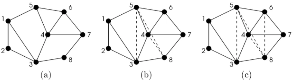
As early as 1961, Parter [26] presented an algorithm, known as Elimination Game (EG), which simulates Gaussian elimination on graphs by repeatedly choosing a vertex and adding edges to make its neighborhood into a clique be-fore removing it, thus introducing the connection between sparse matrices and graphs. In view of the results of [14], the class of graphs produced by EG is exactly the class of chordal graphs. Thus when the given graph is not chordal, Gaussian elimination and EG correspond to embedding it into a chordal graph by adding edges, a process called triangulation. As can be observed on the example in Figure 1, the number of fill edges in the resulting triangulation is heavily dependent on the order in which EG processes the vertices. This order-ing of the graph corresponds to the pivotal orderorder-ing of the rows and columns in Gaussian elimination.
As mentioned above, it is of primary importance to add as few edges as possible when running EG. The corresponding problem is that of computing a minimum triangulation, which is NP-hard [35]. It is possible to compute in polynomial time a triangulation which is minimal, meaning that an inclusion-minimal set of edges is added [24], [31]. However, such a triangulation can be far from minimum, as can be seen from the example of Figure 1(b). In fact, it is easy to see that this example can be extended to a graph with O(n) edges and an O(n2) size fill, whereas a unique fill edge can be obtained by EG on this
graph.
As a result, researchers have resorted to heuristics, of which one of the most universally used and studied is Minimum Degree (MD): this runs EG by choosing at each step a vertex of minimum degree in the transitory elimination graph, as illustrated by Figure 1(d). This algorithm is widely used in practice, and it is known to produce low fill triangulations. In addition, MD is also observed [6] to produce triangulations which are often minimal or close to minimal.
MD has given rise to a large amount of research with respect to improving the running time of its practical implementations, and the number of papers written on this subject is in the hundreds [1, 16]. However, very little is proved about its quality. It has in fact been analyzed theoretically only to a limited
(a) (b) (c) (d) 4 6 7 4 1 2 6 7 5 3 3 2 5 1 6 7 4 3 2 5 1
Figure 1: (a) A graph G, and various triangulations of G by EG through the given orderings: (b) A minimal triangulation with O(n2) fill edges. (c) A
non-minimal triangulation of G with less fill. (d) A minimum triangulation of G.
extent, which makes it difficult to gain control over this heuristic in order to improve it yet further, although recent research has been done on algorithms for low fill minimal triangulations [6, 10, 27].
In this paper, we use recent graph theoretical results on minimal triangula-tion and minimal separators to explain, at least in part, why MD yields such good results. In fact, it turns out that one of the reasons why MD works so well is that the EG algorithm is remarkably robust, in the sense that it is resilient to error: if at some step of the process an undesirable edge with respect to minimal triangulation is added, at later steps the chances of adding only desirable edges remain intact. During EG, and in particular MD, we are able to identify the fill edges that are safe to add with respect to a minimal triangulation. Thus we show how to use EG to compute a partial minimal triangulation. We also show the implementation details of how to compute this partial minimal triangulation efficiently. An interesting property of this partial minimal triangulation is that when it is completed in any way to a minimal triangulation the resulting graph is a minimal triangulation of the input graph and a subgraph of the filled graph resulting from EG.
One of the strengths of this approach is its parallel nature, and we give implementation details for both a sequential and a parallel version of it. This results in the first efficient parallel algorithm for computing minimal triangula-tions sandwiched between the input graph and the filled graph resulting from EG.
Furthermore, we use the insight we have gained on the mechanisms which govern EG, and in particular MD, to propose a new algorithm that improves the results obtained by MD, giving minimal triangulations with low fill.
The remainder of this paper is organized as follows: Section 2 gives the graph theoretic background, introduces EG formally, and gives previous results on minimal separators and minimal triangulation. In Section 3, we show that EG can be used to compute a partial minimal triangulation, thereby giving some new invariants for EG. In Section 4, we explain how to implement this efficiently both sequentially and in parallel. Section 5 proposes new algorithms to compute minimal triangulations using EG. In particular we show how to extend a partial minimal triangulation to a minimal triangulation in parallel, thereby solving the sandwiched minimal triangulation problem in parallel. Section 6 applies our new results to MD, and uses our new insight to give some explanations as to the remarkably good behavior of MD.
2
Preliminaries
Given a graph G = (V, E), we denote n = |V | and m = |E|. For any subset S of V , G(S) denotes the subgraph of G induced by S. For the sake of simplicity, we will use informal notations such as H = G + {e} + {x} when H is obtained from G by adding edge e and vertex x. For any vertex v of G, NG(v) denotes the
neighborhood of v in G, and NG[v] denotes the set NG(v) ∪ {v}. For a given set
of vertices X ⊂ V , NG(X) = ∪v∈XNG(v) − X, and NG[X] = ∪v∈XNG(v) ∪ X.
We will omit the subscripts when there is no ambiguity.
A vertex is simplicial if its neighborhood is a clique. We will say that we saturate a set of vertices X when we add to the graph all the edges necessary to make X into a clique. A graph is chordal, or triangulated, if it contains no chordless cycle of length ≥ 4. A chordal graph H = (V, E + F ) is called a triangulation of G = (V, E), where G is an arbitrary graph. The set F of edges which are added to obtain a triangulation is called a fill. A triangulation H is minimal if no strict subset of F can be added to G to obtain a triangulation.
A bijective function α : V → {1, 2, ..., n} is called an ordering of the vertices of G = (V, E), and (G, α) will denote a graph G, the vertices of which are ordered according to α. We will use α = (v1, v2, ..., vn), where α(vi) = i.
The algorithmic description of Elimination Game (EG) given below defines the notations we will use in the rest of this paper:
Algorithm Elimination Game (EG)
Input: A graph G = (V, E), and an ordering α of the vertices in G. Output: A triangulation G+
α of G.
G1
α← G; G+α ← G;
fork = 1 to n do
Let F be the set of edges necessary to saturate NGk
α(vk) in G k α; Gk+1 α ← Gkα+ F − {vk}; G+α ← G+α + F ; We note Gk
α = (Vαk, Eαk), where Vαk = {vk, ..., vn}. According to the
defini-tion used in [24], we will call Gk
α(Vαk− NGk
α[vk]) the section graph at step k. A
characterization of the edges of G+
α is given in [31], which easily extends to Gkα.
Lemma 2.1 ([31]) Let α = (v1, ..., vn) and let i, j be distinct integers in [1, n]
(resp. [k, n]). Then vivj is an edge of G+α (resp. Gkα) iff there is a path in
G between vi and vj (possibly reduced to one edge), all intermediate vertices of
which have a number which is strictly smaller than min{i, j} (resp. k) in α. If no fill edges are produced during EG (i.e, if G+
α = G) then α is called a
perfect elimination ordering (peo) of G. Fulkerson and Gross showed in [14] that a graph is chordal iff it has a peo. Consequently, since α is a peo of G+
α, EG is an
algorithm for computing triangulations (not necessarily minimal). In [24] it is shown that any minimal triangulation of G can also be generated by EG. Thus for each minimal triangulation H of G, there exists an ordering α on G such that H = G+
α. Such an ordering α is called a minimal elimination ordering. If
a given ordering α is not minimal, we will call a minimal triangulation H of G that is a subgraph of G+α, a sandwiched minimal triangulation.
The Minimum Degree (MD) heuristic is based on EG: it takes as input an unordered graph G, and computes an ordering α along with the corresponding
triangulation G+
α, by choosing at each step a vertex of minimum degree in Gkα
and numbering it as vk.
Minimal separators are central to chordal graphs and minimal triangulations. Given a graph G = (V, E), a vertex set S ⊂ V is a separator if G(V − S) is disconnected. If G(V − S) has a connected component C such that NG(C) = S
then C is called a full component of S in G. A separator S is a minimal separator of G if S has at least two full components in G.
Characterization 2.2 (Dirac [13]) A graph is chordal iff all its minimal sep-arators are cliques.
The idea behind the connection between minimal separators and minimal triangulations is that forcing a graph into respecting Dirac’s characterization will result in a minimal triangulation, by repeatedly choosing a not yet processed minimal separator and saturating it [2, 19, 25]. We will need the definition of crossing separators, which characterize the separators that disappear when a saturation step of this process is executed:
Definition 2.3 ([19]) Let S and S′
be two minimal separators of G. S and S′ are said to be crossing if there exist two connected components C
1, C2 of
G(V − S), such that S′∩ C
1 6= ∅ and S′∩ C2 6= ∅ (the crossing relation is
symmetric).
The saturation process described above can be generalized by choosing and simultaneously saturating a set of pairwise non-crossing minimal separators in-stead of a single minimal separator at each step, until a chordal graph is ob-tained. We will refer to this generalized process as the Saturation Algorithm. Given a set S of minimal separators of G, we will denote GS the graph obtained
from G by saturating all the separators belonging to S .
The following results from the works of Kloks, Kratsch and Spinrad [19] and Parra and Scheffler [25] provide a proof of this algorithm and will be used in Sections 3 and 5.
Theorem 2.4 ([19, 25]) A graph H = (V, E + F ) is a minimal triangulation of G = (V, E) iff there is a maximal set S of pairwise non-crossing minimal separators of G such that H = GS.
Corollary 2.5 A graph H = (V, E + F ) is a minimal triangulation of G = (V, E) iff H is chordal and there is a set S of pairwise non-crossing minimal separators of G such that H = GS.
Lemma 2.6 ([25]) Let G = (V, E) be a graph, let S and S′ be sets of pairwise
non-crossing minimal separators of G and GS, respectively. Then S ∪ S′ is a
set of pairwise non-crossing minimal separators of G and GS.
Lemma 2.7 ([25]) Let G = (V, E), be a graph and S a set of pairwise non-crossing minimal separators of G. Then any minimal triangulation of GS is a
minimal triangulation of G.
We will also use the notion of substar, which was introduced by Lekkerkerker and Boland [20] in connection with their characterization of chordal graphs.
Definition 2.8 ([20]) Given a graph G = (V, E) and a connected subset X of V , the substars of X are the neighborhoods of the connected components of G(V − N [X]). Note that each substar of X is included in N (X).
When X is reduced to a single vertex x, we will say substar of x for substar of {x}. In fact, although Lekkerkerker and Boland seemed not to be aware of this, the set of substars of some vertex x is exactly the set of minimal separa-tors included in the neighborhood of x. Ohtsuki et al. [24] gave the following characterization of a meo.
Characterization 2.9 [24] An ordering α of V is a meo of a graph G if and only if for every integer k between 1 and n, every fill edge added at step k of EG on (G, α) has both endpoints in some common substar of vk in Gkα.
LB-simpliciality of a vertex was defined in [4] in the following way for more convenient terminology.
Definition 2.10 A vertex x is LB-simplicial if every substar of x is a clique. This was implicitly used by [20] to characterize chordal graphs as graphs in which every vertex is LB-simplicial, but the notion of substar is also very useful in the context of minimal triangulation, because it provides a fast and easy way of repeatedly finding sets of pairwise non-crossing minimal separators when running the Saturation Algorithm. This is fully described in [4], with in particular the following lemma:
Lemma 2.11 ([4]) The substars of a vertex x in a graph G are pairwise non-crossing minimal separators of G.
This resulted in the following algorithm for computing minimal triangula-tions.
Algorithm LB-Triang
Input: A graph G = (V, E), and an ordering α of the vertices in G. Output: A minimal triangulation GLB
α of G.
GLB,1 α ← G;
fork = 1 to n do
Let F be the set of edges necessary to saturate the substars of vk in GLB,kα ;
GLB,k+1
α ← GLB,kα + F ;
GLB
α ← GLB,n+1α ;
We recall here some properties of Algorithm LB-Triang proved in [4]. Items a) to e) of Property 2.12 respectively are or immediately follow from Lemma 4.5 and its proof, Invariant 4.7, Lemma 5.2, Theorem 5.6’s proof, Theorem 5.6 and Corollary 5.7 of [4].
Property 2.12 [4] Let G = (V, E) be a graph, α be an ordering of V and k be an integer between 1 and n.
a) vk has the same neighborhood and substars in GLB,kα and in GLBα .
b) For any integer i between 1 and k, vi is LB-simplicial in GLB,k+1α .
c) Removing LB-simplicial vertices from G does not modify the fill computed by LB-Triang on (G, α).
d) Any fill edge added at step k of LB-Triang on (G, α) is an edge of Gk+1 α .
e) GLB
For an efficient implementation of Algorithm LB-Triang, a useful structure called tree decomposition was used. We will also use it here for the implemen-tation of our algorithms.
Finally, we will mention a result which will be used to prove some of our results. Given a chordal graph G and a peo α of G, Rose [28] showed that every minimal separator of G appears as the neighborhood of a vertex to be processed at some step of EG with ordering α on G. However, there may be some steps such that the neighborhood of the processed vertex of that step is not a minimal separator of G.
Theorem 2.13 ([28]) Let G be a chordal graph and let α = (v1, v2, ..., vn) be
a peo of G. Consider any minimal separator S of G. Then S = NGk
α(vk) for
some k between 1 and n.
3
EG defines a partial minimal triangulation
We will now examine how EG behaves with respect to the minimal separators of the graph which is to be triangulated. We will first extend the definition of a substar of G given in Section 2 to that of a substar of (G, α).
Definition 3.1 Given (G = (V, E), α), we will say that a set S ⊂ V of vertices is a substar of (G, α) if there is some step k of EG such that S is a substar of vk in Gkα, which will be referred to as a substar defined at step k of EG.
Clearly, during the execution of the EG, at each step k, making the currently processed vertex vk simplicial will saturate these substars, and may also add
some extraneous edges which do not have both endpoints in some common substar, so that two kinds of edges can be added:
• Edges which have both endpoints in some common substar defined at step k. We will refer to these edges as substar fill edges.
• Edges which do not have both endpoints in some common substar defined at step k. We will refer to these as extraneous edges.
In Section 2, we mentioned that in G and for a given vertex v, the substars of v are the minimal separators included in the neighborhood of v. One of our most interesting discoveries is that, in fact, all the substars defined by EG are minimal separators of the input graph, whether or not extraneous edges have been added at earlier steps. This fact is stated in Theorem 3.3, and its proof is based on the following theorem, which is interesting in its own right, as it describes a strong correspondence between the structures of G and Gk
α.
Theorem 3.2 Given (G = (V, E), α) and an integer k ∈ [1, n], let Gk α =
(Vk
α, Eαk) and S ⊆ Vαk. The connected components of Gkα(Vαk− S) are the sets
C ∩ Vk
α where C is a connected component of G(V − S) such that C ∩ Vαk 6= ∅,
with the same neighborhoods, i.e. NGk α(C ∩ V
k
α) = NG(C).
Proof. Let CG(S) denote the set of connected components of G(V − S). Let
S ⊆ Vk
α. We have to prove that CGk
α(S) = {C ∩ V
k
α, C ∈ CG(S) | C ∩ Vαk6= ∅}
and ∀C ∈ CG(S) such that C ∩Vαk 6= ∅, NGk α(C ∩V
k
such that C ∩ Vk
α 6= ∅ and let C ′
= C ∩ Vk
α. Let us show that C ′ ∈ C Gk α(S) and NGk α(C ′ ) = NG(C). Gkα(C ′
) is connected because for any vertices x and y in C′
, there is a path P in G(C) between x and y, and by Lemma 2.1, the sub-sequence of P containing only the vertices belonging to Vk
α is a path in Gkα(C ′
) between x and y. Let us show that NGk
α(C ′ ) ⊆ NG(C). Let x ∈ NGk α(C ′ ) and y ∈ C′ such that xy ∈ Ek
α. By Lemma 2.1, there is a path in G between
x and y, all intermediate vertices of which belong to V − Vk
α, and therefore
belong to V − S and consequently belong to C, so x ∈ NG(C). Let us show
that NG(C) ⊆ NGk α(C
′
). Let x ∈ NG(C) and y ∈ C such that xy ∈ E. As
C′ 6= ∅, we may choose z ∈ C′
. Let P be a path in G(C) between y and z and let z′
be the first vertex of P from y belonging to Vk
α. Vertex z ′ ∈ C′ , and by Lemma 2.1 xz′ ∈ Ek α, so x ∈ NGk α(C ′ ). Thus NGk α(C ′ ) = NG(C). As C′ 6= ∅, C′ ⊆ Vk α − S, Gkα(C ′ ) is connected and NGk α(C ′ ) = NG(C) ⊆ S, it follows that C′ ∈ CGk α(S). Therefore, {C ∩ V k α, C ∈ CG(S) | C ∩ Vαk 6= ∅} ⊆ CGk α(S).As ∪C∈CG(S)(C ∩ V k
α) = Vαk− S, the reverse inclusion holds too.
Theorem 3.3 Every substar of (G, α) is a minimal separator of G.
Proof. Let S be a substar defined at step k. S is a minimal separator of Gk α,
and by Theorem 3.2, there are at least as many full components of S in G as in Gk
α. So S is also a minimal separator of G.
Theorem 3.4 The set of substars of (G, α) forms a set of pairwise non-crossing minimal separators of G.
Proof. Let S and S′ be two substars of (G, α) defined at steps k and k′
respectively, with k ≤ k′. By Theorem 3.3, they are both minimal separators of
G. Let us show that they are non-crossing in G. If k = k′ then they are
non-crossing in Gk
α by Lemma 2.11, so they are non-crossing in G by Theorem 3.2.
We suppose now that k < k′
. S is a clique of Gk+1 α and S ′ ⊆ Vk+1 α , so there is a connected component C of Gk+1 α (Vαk+1− S ′ ) such that S ⊆ S′ ∪ C. By Theorem 3.2, there is a connected component C′
of G(V − S′
) containing C, so S ⊆ S′∪ C′
. Hence S and S′
are non-crossing in G.
Note that this theorem does not guarantee that the set of substars defines a set of pairwise non-crossing minimal separators which is maximal. For instance, for any non complete graph G, if v1 is a universal vertex of G, then there is no
substar of (G, α), whereas G has at least one minimal separator. A less trivial counterexample is given in Figure 2(b) of Example 3.5.
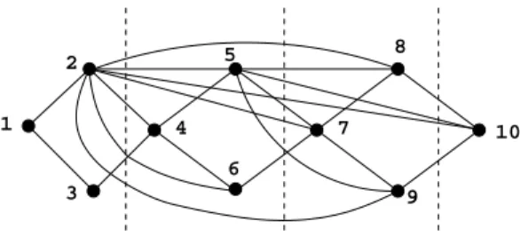
Example 3.5 Figure 2 shows two executions of EG on graph G. A graph G and an ordering α are given in (a). The minimal separators of G are: {1, 3}, {3, 5}, {3, 7}, {1, 4, 6}, {1, 4, 7}, {1, 4, 8}, {3, 5, 7}, {4, 5, 7}, {4, 5, 8}, {4, 6, 8}, {3, 4, 6}. We now demonstrate the execution of EG on (G, α) resulting in the graph shown in (b).Step 1: N (1) = {2, 3, 5}, C1= {4, 6, 7, 8}, N (C1) = {3, 5};
substar fill edge 35 and extraneous edge 25 are added. Step 2: N (2) = {3, 5}; C2= {4, 6, 7, 8}, N (C2) = {3, 5}; 2 is simplicial, so no edge is added. Step 3:
N (3) = {4, 5, 8}, C3= {6, 7}, N (C3) = {4, 5, 8}; substar fill edges 48 and 58 are
added. Step 4: N (4) = {5, 6, 7, 8}; 4 is universal, so no component is defined; extraneous edges 57 and 68 are added; the remaining graph becomes a clique;
1 2 3 4 5 6 7 8 1 2 3 4 5 6 7 8 6 7 5 3 4 8 2 1 (a) (b) (c)
Figure 2: Two executions of EG on the same graph G with (b) an arbitrary ordering, and (c) an MD ordering. (b) is a triangulation of G which is not minimal, (c) is in this case a minimum triangulation of G.
no further edge is added. The set of substars of (G, α) is thus {{3, 5}, {4, 5, 8}}, which is a set of pairwise non-crossing minimal separators of G, but not a max-imal one as {{3, 5}, {4, 5, 8}, {4, 5, 7}} and {{3, 5}, {4, 5, 8}, {4, 6, 8}} are also sets of pairwise non-crossing minimal separators of G. If only substar fill edges are preserved, a chordless cycle 5678 remains in the graph thus obtained. In order to saturate a maximal set of pairwise non-crossing minimal separators of G, {4, 5, 7} or {4, 6, 8} should also be saturated. On the same graph, MD yields a minimal (and even minimum) triangulation, as shown in (c).
Thus by Theorem 3.4 and Lemma 2.7, a minimal triangulation of a given graph G can be computed as follows. Run EG on (G, α) where α is an ordering of V , then remove from G+
α all fill edges that do not appear within substars
(i.e., the extraneous fill edges). As Example 3.5 shows, the resulting graph is not necessarily chordal, but any minimal triangulation of it will be a minimal triangulation of G. Furthermore, this minimal triangulation will be a subgraph of G+
α, as we will show in Section 5. In Section 4, we will show how to
com-pute this partial minimal triangulation both in O(nm) sequential time and in O(log2n) parallel time on O(nm) processors, and in Section 5 we will show how to complete it to a minimal triangulation of G in O(log3n) parallel time on O(nm) processors.
We would like to end this subsection with a discussion on the robustness of EG regarding the process of defining non-crossing minimal separators of G. If, during the EG process, no extraneous edge is added, then the triangulation which is computed is minimal. However, due to Theorem 3.4, even when extra-neous edges have been added, all substar fill edges added later belong to a set of pairwise non-crossing minimal separators of G, and therefore to a minimal triangulation of G. Thus if only a few extraneous edges are added during EG process, they will not destroy the property that all the substar fill edges are “useful” edges and that these few extraneous edges are the only “unnecessary” edges introduced. This makes EG a fault-tolerant procedure.
3.1
Using G
+αto compute the substars of
(G, α).
In this subsection, we will show that it is not necessary to compute the substars during the course of EG on (G, α). We can indeed compute the substars from only G and the filled graph G+
α. This is interesting since given (G, α), the filled
graph G+
Tarjan and Yannakakis in [32], whereas EG requires O(n3) time. We will look
at the minimal separators of G+
α, and show how to split these into the desired
substars of (G, α). The results of this subsection are needed for the O(nm) time implementation that will be given in the next section.
In the following, we suppose that a graph G = (V, E) and an ordering α = (v1, v2, ..., vn) of V are given.
Lemma 3.6 Let S be a minimal separator of G+
α. Then there are an integer k
between 1 and n and a full component C0 of S in G such that S = NGk
α(vk) and
C0∩ Vαk = {vk}.
Proof. As α is a peo of G+
α, by Theorem 2.13 there is an integer k between
1 and n such that S = N(G+
α)kα(vk), and (G
+
α)kα = G+α(Vαk). Since we also have
NG+
α(Vαk)(vk) = NG k
α(vk), we get S = NGkα(vk). As {vk} is a full component
of S in Gk
α, by Theorem 3.2 there is a full component C0 of S in G such that
C0∩ Vαk = {vk}.
Definition 3.7 A subset S of V is a split-minsep of (G, α) if there is a minimal separator S′ of G+
α and a full component C0 of S′ in G such that S is a substar
of C0 in G (S is said to be derived from S′).
It follows from Lemma 3.6 that every minimal separator of G+
α can be split
into split-minseps of (G, α).
Remark 3.8 In the definition of a split-minsep of (G, α), we can moreover assume that there is an integer k between 1 and n such that S′= N
Gk
α(vk) and
C0∩ Vαk = {vk}.
Proof. Let S be a split-minsep of (G, α). Let S′
be a minimal separator of G+α
and C′
0be a full component of S
′ in G such that S is a substar of C′
0in G. Let
C be a component of G(V − NG[C0′]) defining S, i.e. such that S = NG(C). By
Lemma 3.6 there is an integer k between 1 and n and a full component C0 of
S′ in G such that S′= N Gk
α(vk) and C0∩ V
k
α = {vk}. Then S is also a substar
of C0 in G: it is evident if C 6= C0, otherwise S is the substar of C0 defined by
C′
0, as S = NG(C) = NG(C0) = S′ = NG(C0′), with C0= C 6= C0′.
Lemma 3.9 Let C0 be a non-empty subset of V such that G(C0) is connected.
Then the substars of C0 in G are exactly the minimal separators of G included
in NG(C0).
Proof. Let S be a substar of C0 in G. Then S is the neighborhood of some
connected component C of G(V − N [C0]). So S ⊆ N (C0), and as C and the
component of G(V − S) containing C0are two distinct full components of S in
G, S is a minimal separator of G.
Conversely let S be a minimal separator of G included in N (C0). Then there is a
component C′
0of G(V − S) containing N [C0] − S. Let C′ be a full component of
S in G different from C′
0. As C′⊆ V − N [C0], C′is a subset of some component
C of G(V − N [C0]). But as C ⊆ V − N [C0] ⊆ V − S, C is a subset of some
component of G(V − S). Hence C = C′
, S = N (C′
) = N (C) and S is a substar of C0 in G.
Lemma 3.10 A subset S of V is a split-minsep of (G, α) if and only if it is a minimal separator of G included in some minimal separator of G+
α.
Proof. By Lemma 3.6 every minimal separator S of G+
α is in the form NG(C0),
where C0is a non-empty subset of V such that G(C0) is connected. We conclude
with Lemma 3.9.
Lemma 3.11 Let k be an integer between 1 and n, let S ⊆ Vk
α and let C0 be
a full component of S in G such that C0∩ Vαk = {vk}. Then C0 is also a full
component of S in G+ α.
Proof. As G is a subgraph of G+
α, C0 is a non-empty connected subset of
vertices in G+
α with S ⊆ NG+α(C0). It remains to show that NG +
α(C0) ⊆ S. By
Theorem 3.2 every fill edge having one of its endpoints in C0inserted before or
at step k of EG has its other endpoint in NG[C0], and no fill edge having one of
its endpoints in C0 can be inserted after step k since C0 is eliminated. Hence
NG+
α(C0) ⊆ S.
Lemma 3.12 Let k be an integer between 1 and n, let S ⊆ Vk
α and let C0 be a
full component of S in G such that C0∩ Vαk= {vk}. Then any substar of C0 in
G is a split-minsep of (G, α).
Proof. Let S1 be a substar of C0 in G defined by a component C of G(V −
NG[C0]). By Lemma 3.11 C0is also a full component of S in G+α. Let S ′ 1be the
substar of C0 in G+α defined by the component of G+α(V − NG[C0]) containing
C. S1⊆ S′1, and by Lemma 3.9 S1and S1′ are minimal separators of G and G+α
respectively. We conclude with Lemma 3.10.
Theorem 3.13 The set of all split-minseps of (G, α) is exactly the set of all substars of (G, α).
Proof. Let S be a split-minsep of (G, α). Let S′
be a minimal separator of G+ α
and C0be a full component of S′ in G such that S is a substar of C0in G. Let
C be a component of G(V − NG[C0]) such that S = NG(C). By Remark 3.8
we can moreover assume that there is an integer k between 1 and n such that S′ = N Gk α(vk) and C0∩ V k α = {vk}. First case : C ∩ Vk α 6= ∅.
By Theorem 3.2, S is the substar of (G, α) defined at step k by C ∩ Vk α. Second case : C ∩ Vk α = ∅. Let k′ = max{α(v), v ∈ C}. k′ < k, so S ⊆ Vk′ α and C0∩ Vk ′ α 6= ∅. By Theorem 3.2 S = NGk′
α(vk′) and S is the substar of (G, α) defined at step k
′ by the component of Gk′ α(Vk ′ α − S) containing C0∩ Vk ′ α .
Conversely, let S be a substar of (G, α) defined at step k, and let Sk = NGk α(vk).
By Theorem 3.2 there is a full component C0of Skin G such that C0∩Vαk= {vk}
and such that S is a substar of C0in G. By Lemma 3.12 S is a split-minsep of
(G, α).
Thus, by Theorem 3.13 we do not need to execute EG to compute the set of substars of (G, α). It is sufficient to compute the split-minseps derived from all minimal separators of G+
3.2
Relationships between EG and LB-Triang
LB-Triang resembles EG as it processes the vertices in a given ordering α and adds fill edges in their neighborhood. Furthermore, the processed vertices can be removed from the graph just like in EG [4]. However, whereas EG saturates the whole neighborhood of vertex vk at step k, LB-Triang saturates only the
substars of vk in the current graph. As LB-Triang always computes a minimal
triangulation, it is interesting to compare the substars computed during LB-Triang to the substars of (G, α).
1 2 3 4 5 6 7 8 1 2 3 4 5 6 7 8 1 2 3 4 5 6 7 8 (a) (b) (c)
Figure 3: (a) Graph G with ordering α, (b) graph GS, where S is the set of
substars of (G, α) and (c) graph GLB
α . (b) is a partial minimal triangulation of
G, (c) is a minimal triangulation of G.
Example 3.14 Consider graph G and the ordering α of Figure 2. The graph GS obtained from G by saturating the substars of (G, α) and the graph GLBα are
shown in Figure 3. The substars of (G, α) are: {3, 5}, defined for the first time at Step 1 (and redefined at Step 2) and {4, 5, 8}, defined at Step 3. They are also substars defined by LB-Triang process: {3, 5} is also defined for the first time at Step 1 (and redefined at Step 4) and {4, 5, 8} is also defined for the first time at Step 3 (and redefined at step 6). Note that LB-Triang also defines the substars {1, 3}, {4, 6, 8} (adding the fill edge 68 at Step 5) and {3, 4, 5} that are not substars of (G, α).
We have the following result.
Theorem 3.15 Let S be a substar of (G, α) defined for the first time at step k. Then S is a substar of vk defined by LB-Triang process on (G, α) for the first
time at step k.
Proof. Let G = (V, E) be a graph, and let α = (v1, ..., vn) be an ordering
of V . For any k between 1 and n + 1, let Hk = GLB,kα . We will use the
following Lemmas. Lemma 3.16 is a well-known property of chordal graphs, and Lemma 3.17 easily follows from the definition of an LB-simplicial vertex and immediately follows from Lemma 5.1 of [4].
Lemma 3.16 Let C0 be a non-empty subset of V . If G is chordal, G(C0) is
connected and N (C0) is a clique of G then there is a vertex v of C0 such that
N (C0) ⊆ N (v).
Lemma 3.17 A vertex v of G is LB-simplicial in G if and only if v belongs to no chordless cycle in G of length at least 4.
Let S be a substar of (G, α) defined for the first time at step k by a com-ponent C of Gk
α(Vαk− Sk), where Sk = NGk
α(vk). By Theorem 3.2 there is a
full component C0 of Sk in G such that C0∩ Vαk = {vk} and there is another
component C′
of G(V − Sk) such that C′∩ Vαk = C and NG(C′) = S. For any
i between 1 and k + 1, C0and C′ are also components of Hi(V − Sk) with the
same neighborhoods, i.e. NHi(C0) = Sk and NHi(C
′
) = S. We prove this for C0 (the argument is similar for C′). Hi(C0) is connected and Sk ⊆ NHi(C0)
because G ⊆ Hi, and NHi(C0) ⊆ Sk because every edge of Hi having one of its
endpoints in C0is an edge of Gjαfor some j ≤ i by Property 2.12 d), and
there-fore has its other endpoint in NG[C0] = C0∪ Sk by Theorem 3.2. In particular,
for any i between 1 and k, S is a substar of C0 in Hi and of C0∩ Vαi in Giα, so
by Lemma 3.9 S is a minimal separator of both Hi and Giα.
Let us show that S is a clique of Hk+1. We suppose for contradiction that
it is not the case. Let y, z be non-adjacent vertices of S in Hk+1, let P1 and
P2 be chordless paths in Hk+1 between y and z whose internal vertices are in
C0 and C′ respectively, and let Q be the cycle formed by P1 and P2. Q is a
chordless cycle in Hk+1 of length at least 4 containing some vertex v of C0. As
C0∩ Vαk= {vk}, v = vi for some i ≤ k. By Property 2.12 b), v is LB-simplicial
in Hk+1, and by Lemma 3.17 v belongs to no chordless cycle in Hk+1 of length
at least 4, a contradiction.
Now consider the graph H = Hk+1(C0∪ S). C0 is non-empty, H(C0) is
con-nected, NH(C0) = S is a clique of H and H is chordal since by the preceding
argument no vertex of C0 belongs to a chordless cycle in Hk+1, and therefore
in H, of length at least 4, and S is a clique of H. So by Lemma 3.16 there is a vertex v of C0 such that S ⊆ NH(v), and therefore there is some i ≤ k
such that S ⊆ NH(vi). Let i be the smallest such integer, and let us show that
i = k. By Property 2.12 d) no fill edge containing vi can be added after step i
of LB-Triang, so S ⊆ NH(vi) ⊆ NHk+1(vi) = NHi(vi), and by Property 2.12 d)
again S ⊆ NHi(vi) ∩ V i α⊆ NGi α(vi). As S is minimal separator of G i α included in NGi
α(vi), by Lemma 3.9 S is a substar of (G, α) defined at step i, and since
S is defined for the first time at step k, i = k. As S is minimal separator of Hk
included in NHk(vk), by Lemma 3.9 S is a substar of vk defined by LB-Triang
process at step k, and it is defined for the first time at step k since for any i < k, S 6⊆ NH(vi) and therefore S 6⊆ NHi(vi).
Theorem 3.18 Let S be the set of substars of (G, α). GS ⊆ GLBα ⊆ G+α and
if α is a meo of G then GS = GLBα = G+α.
Proof. By Theorem 3.15 GS ⊆ GLBα , by Property 2.12 e) GLBα ⊆ G+α, and
if α is a meo of G then by Characterization 2.9 every fill edge in G+ α. has
both endpoints in some common substar of (G, α), so G+
α ⊆ GS, and therefore
GS = GLBα = G+α.
Note that if α is not a meo of G then by Property 2.12 e) GLB
α ⊂ G+α, but
GS may be equal to GLBα . In particular, if G is chordal and α is not a peo of
4
Computing the partial minimal triangulation
efficiently
In this section we will give the implementation details of how to compute and saturate the substars efficiently. More formally, given (G, α), we want to com-pute GS, where S is the set of substars of (G, α). We give both a sequential
and a parallel implementation of this process. In both implementations, we will use the definition of a substar of (G, α) as a split-minsep of (G, α) described in Subsection 3.1.
4.1
Partial minimal triangulation in sequential O(nm) time
In this subsection, we will show that the set S of all substars of (G, α) and the graph GS can be computed in O(nm) time. For this second result, we will use adata structure introduced in [4] to implement LB-Triang and we will prove more generally that for any given set S of pairwise non-crossing minimal separators of G, the graph GS can be computed in O(nm) time.
Theorem 4.1 Given (G, α), the set S of all substars of (G, α) can be computed in O(nm) time.
Proof. By Theorem 3.13 it is sufficient to compute the set of split-minseps of (G, α). Computing G+
α can be done in time O(n + m ′
), where m′
is the number of edges of G+
α, as described in [32]. Since it is a chordal graph, it has
at most n minimal separators (by Theorem 2.13) which can be computed in a global O(n + m′
) time [7]. For any minimal separator S′
of G+
α, the connected
components of G(V −S′
) and their neighborhoods can be computed in O(n+m) time. The split-minseps derived from S′
are these neighborhoods, except S′
itself if it has only one full component in G. We use a Search/Insert data structure similar to that used in [4] to eliminate duplicates with no extra time cost, and we obtain a global O(nm) time bound.
It is less easy to prove that saturating the substars of (G, α) can also be done in O(nm) time. With a straightforward implementation, saturating a substar takes O(m′) time, where m′ is the number of edges of G
S. As the
number of substars of (G, α) is bounded by n (by Lemma 4.2 below) saturating all substars takes O(nm′) time. To achieve O(nm) time, we will use the tree
decomposition data structure used in [4] to compute GLB
α and will extend it
to the more general problem of computing GS for any set S of pairwise
non-crossing minimal separators of G.
Lemma 4.2 For any set S of pairwise non-crossing minimal separators of G, |S | ≤ n.
Proof. Let S′
be a maximal set of pairwise non-crossing minimal separators of G containing S . GS′ is chordal by Theorem 2.4, and by Lemma 2.6 S′ is
also a set of minimal separators of GS′. As by Theorem 2.13 chordal graph
GS′ has at most n minimal separators, we obtain |S | ≤ |S′| ≤ n.
Theorem 4.3 Given a graph G and a set S of pairwise non-crossing minimal separators of G, the partial minimal triangulation GS of G can be computed in
Proof. We generalize the implementation of LB-Triang described in [4] using a data structure called tree decomposition by minimal separators. We recall the definition of this structure.
A tree structure on G is a structure T S = (T, (Xu)u∈UT, (Suv)uv∈ET), where
T = (UT, ET) is a tree, Xuis a subset of V for each u in UT and Suv is a subset
of V for each uv in ET.
We note:
- ∀x ∈ V , Ux= {u ∈ UT | x ∈ Xu} and Tx= T (Ux) = (Ux, Ex),
- ∀C ⊆ V , TC= (∪x∈CUx, ∪x∈CEx) = (UC, EC),
- ∀uv ∈ ET, Tuv and Tvu are the two connected components of T′= (UT, ET \
{uv}) respectively containing u and v.
A tree decomposition of G is a tree structure T S on G such that: a) ∪u∈UTXu= V ,
b) ∀xy ∈ E, ∃u ∈ UT | x, y ∈ Xu (i.e. Ux∩ Uy 6= ∅),
c) ∀x ∈ V, Txis a subtree of T ,
d) ∀uv ∈ ET, Suv = Xu∩ Xv.
If T S is a tree decomposition of G, and C is a connected subset of V then TC
is a subtree of T [4].
A tree decomposition of G by minimal separators is a tree decomposition T S of G verifying the extra property:
e) ∀uv ∈ ET, ∃C1, C2full components of Suv in G | TC1⊆ Tuv and TC2 ⊆ Tvu.
The graph GS can be computed as follows. First a tree decomposition of G by
minimal separators T S is computed, where the edges of T contain the elements of S (or more accurately, the elements of a subset S′ of S such that every
separator in S is a subset of a separator in S′, so that G
S = GS′). Then, using
Algorithm Neighbors described in [4], we compute the closed neighborhood in GS′, and therefore in GS, of every vertex of G. The whole process is described
in the following variant NonCrossing-Treedecomp of Algorithm LB-Treedecomp presented in [4]. We refer the reader to [4] for the implementations of Algorithms Neighbors, InitVariables and UpdateVariables. For every vertex x of G, variable u(x) contains an arbitrary node of Tx.
Algorithm Neighbors
Input: A graph G = (V, E), a vertex x of G, and a tree decomposition T S = (T = (UT, ET), (Xu)u∈UT, (Suv)uv∈ET) of G.
Output: the set NG′[x], where G′ is the graph obtained from G by saturating
the elements of the sets Suv for each uv in ET.
Algorithm NonCrossing-Treedecomp Input: A graph G = (V, E),
and a set S of pairwise non-crossing minimal separators of G. Output: the graph GS.
T ← ({u0}, ∅); Xu0 ← V ;
InitVariables(); foreachS ∈ S do
Compute two distinct full components C1 and C2 of S in G;
Pick any vertex c1 in C1 and any vertex c2in C2;
Compute the path P = (u(c1) = u0, u1, ..., up= u(c2))
in T between u(c1) and u(c2);
foreachs ∈ S do
whiles 6∈ Xui doi ← i + 1;
w ← ui;
ifXw∩ C26= ∅ then
Split w into w1 and w2;
Xw1← Xw∩ (C1∪ S); Xw2 ← Xw\ C1;
Replace each edge wv by w1v with Sw1v = Swv if Swv⊆ C1∪ S
and by w2v with Sw2v= Swv otherwise;
Add edge w1w2; Sw1w2 ← S;
UpdateVariables(); GS ← (V, ∅) ;
foreachx ∈ V do
NGS[x] ← Neighbors(G, x, T S);
The main difference between Algorithms LB-Treedecomp and NonCrossing-Treedecomp is the way in which the node w to be split is searched for in T . We first prove the following Lemma, which generalizes Lemmas 7.17 to 7.20 from [4].
Lemma 4.4 Let S ∈ S . We suppose that T S is a tree decomposition of G just before processing S in an execution of NonCrossing-Treedecomp. Then when processing S a node w = ui of T is computed, with S ⊆ Xw, Xw∩ C16= ∅ and
if Xw∩ C2= ∅ then S ⊆ Suiui+1.
Proof. (of Lemma 4.4) Just before processing S, as T S is a tree decomposition of G, TC1 and TC2 are subtrees of T . Moreover |UC1 ∩ UC2| ≤ 1 (otherwise
TC1 and TC2 would have a common edge uv with Suv ∈ S , Suv ∩ C1 6= ∅
and Suv∩ C2 6= ∅, so Suv and S would be crossing elements of S ). Let Q be
the path between TC1 and TC2 in T . Q is in the form (ui1, ui1+1, ..., ui2) with
0 ≤ i1 ≤ i2 ≤ p. For any s ∈ S, s ∈ NG(C1) ∩ NG(C2), so Us∩ UC1 6= ∅ and
Us∩ UC2 6= ∅, and therefore the set of integers j in [0, p] such that s ∈ Xuj is an
interval containing i1 and i2. It follows that the execution of the loop ’foreach
s ∈ S do’ will terminate with 0 ≤ i ≤ i1 and S ⊆ Xi. So S ⊆ Xw and as
0 ≤ i ≤ i1, ui is a node of TC1 and therefore Xw∩ C16= ∅. If Xw∩ C2= ∅ then
i < i2 and therefore S ⊆ Xui∩ Xui+1= Suiui+1.
By Lemma 4.4, if T S is a tree decomposition of G just before processing S then either Xw∩ C26= ∅ and then w is split into w1 and w2 and the edge w1w2
with Sw1w2 = S is created, or S is a subset of an already processed minimal
separator in S . Thus the set S′ of minimal separators contained in the edges
of the final tree T is a subset of S such that GS = GS′, and Algorithm
Neighbors correctly computes the closed neighborhood of every vertex of G in GS, provided that T S is a tree decomposition of G at every step. We prove
that T S is a tree decomposition of G by minimal separators at every step of the algorithm in the same way as in [4] (Invariant 7.21) since this proof only uses the facts that S is a set of pairwise non-crossing minimal separators of G and that if the node w computed when processing S is split then S ⊆ Xw,
Xw∩ C16= ∅ and Xw∩ C26= ∅, which holds by Lemma 4.4. This completes the
proof of correctness of NonCrossing-Treedecomp.
Let us prove O(nm) time bound. We know from [4] that InitVariables requires O(n) time, that splitting a node w, UpdateVariables and Neighbors take O(m)
time (using the fact that T S is a tree decomposition of G by minimal separators), and that the data structure used to implement the sets Xuallows to test whether
a vertex of G belongs to a set Xu or not in O(1) time. Computing C1 and C2
requires O(n + m) time, computing P takes O(n) time (since by Lemma 4.2 |ET| ≤ |S | ≤ n), as well as computing w and testing Xw∩ C26= ∅. Thus each
iteration of each one of the two main foreach-loops requires O(n + m) = O(m) time, and since |S | ≤ n we obtain a global O(nm) time bound.
Corollary 4.5 Given (G, α), the partial minimal triangulation GS of G can
be computed in O(nm) time, where S is the set of all substars of (G, α). Proof. By Theorem 4.1 S can be computed in O(nm) time. By Theorem 3.4 S is a set of pairwise non-crossing minimal separators of G, so we conclude with Theorem 4.3.
Note that the algorithm described by Dahlhaus in [10] as the Tree Splitting Procedure can also be used to compute the set S of substars of (G, α) and the graph GS in O(nm) time. This algorithm computes what is called in [10] a
quasi-minimal tree representation of G. It can be proved that the computed tree is a tree decomposition of G by minimal separators whose edges exactly contain the substars of (G, α). This tree is initialized with a clique tree of G+ α
and at each step of the algorithm, an edge containing a minimal separator S′
of G+
α is split into edges containing some split-minseps of (G, α) derived from S ′
. The graph GS can be computed from that tree, using Algorithm Neighbors in
the same way as in NonCrossing-Treedecomp.
4.2
Parallel partial minimal triangulation
In this subsection, we give a parallel algorithm for computing the substars of (G, α).
Algorithm Parallel Substar Computation (PSC)
Input: A graph G = (V, E) and an ordering α = (v1, v2, ..., vn) of G.
Output: The set of substars of (G, α).
1. Compute the connected components C of G({v1, v2, ..., vi})
for all i ∈ [1, n − 1];
2. Compute NG[C] for all connected components C computed at Step 1;
3. Compute the connected components K of G(V − NG[C]) for all
closed neighborhoods NG[C] computed at step 2;
4. Compute NG(K) for all connected components K computed at step 3;
5. Eliminate duplicates from the sets NG(K) of Step 4 by sorting them;
6. Output the remaining sets from Step 5 as the substars of (G, α);
Lemma 4.6 Algorithm PSC computes the set of all substars of (G, α). Proof. By Theorem 3.13 it is sufficient to show that PSC computes the set of all split-minseps of (G, α).
Let S be a set computed by PSC. Let i ∈ [1, n − 1], let C0 be a component
of G({v1, v2, ..., vi}) and K be a component of G(V − NG[C0]) such that S =
S0 ⊆ Vαi+1 ⊆ Vαk, C0 is a full component of S0 in G such that C0∩ Vαk = {vk}
and S is a substar of C0 in G, so by Lemma 3.12 S is a split-minsep of (G, α).
Conversely let S be a split-minsep of (G, α). By Remark 3.8 there is a minimal separator S′
of G+α, a full component C0of S′ in G and an integer k between 1
and n such that S is a substar of C0 in G, S′ ⊆ Vαk+1 and C0∩ Vαk = {vk}. It
follows that C0is a component of G({v1, v2, ..., vk}), so S is computed by PSC.
Lemma 4.7 Algorithm PSC runs in O(log2n) parallel time with O(nm) pro-cessors on a CREW PRAM.
Proof. The first step of the algorithm can be done as follows. We give any edge vivj the distance d(vi, vj) = max(i, j). Let Ei be the set of edges vw of
G with d(v, w) ≤ i. We call the connected components of Ei the i-clusters. By
[11], for all i simultaneously, the i-clusters can be determined in O(log2n) time with O(n + m) processors. Observe that the i-clusters are just the connected components of G({v1, ..., vi}). The second step can be done in O(log n) time on
O(nm) processors, since for each C separately it can be done in logarithmic time with a linear number of processors and the number of C is bounded by n. The third step can be done in O(log2n) time on O(nm) processors, since it can be done in O(log2n) time with O(n + m) processors, for each C separately, using the algorithm of Shiloach and Vishkin [30] and the number of C is bounded by n. The fourth step is analogous to the second step, it requires the same bounds for each C separately, and therefore the same global bounds. The fifth step needs O(log n) time and O(n) processors if we assume that one comparison needs constant time and a linear number of processors [9]. Here one comparison needs O(n) processors and O(log n) time on a CREW-PRAM. Therefore the fifth step needs O(n2) processors and O(log2n) time on a CREW-PRAM.
Theorem 4.8 Given (G, α), the partial minimal triangulation GS of G can be
computed in parallel O(log2n) time with O(nm) processors on a CREW PRAM, where S is the set of all substars of (G, α).
Proof. By Lemmas 4.6 and 4.7, we know how to compute the substars S of (G, α) in parallel O(log2n) on O(nm) processors. The substar edges can be added to G in parallel O(log n) time on O(nm) processors, and the result follows.
5
Completing the partial minimal triangulation
into a minimal triangulation
Theorem 5.1 Let S be the set of substars of (G, α). Then any minimal tri-angulation H of GS is a minimal triangulation of G which is a subgraph of
G+ α.
Proof. Let H be a minimal triangulation of GS. By Theorem 3.4 and
Lemma 2.7, H is a minimal triangulation of G. Let us show that H is a sub-graph of G+
α. By Theorem 2.4 there is a set S ′
separators of GS such that H = (GS)S′. As GS is a subgraph of G+α, it is
sufficient to show that any element of S′
is a clique of G+
α. Let T ∈ S ′
, let u and v be two vertices of T with α(u) < α(v) and let k = α(u) (i.e. u = vk).
Let us show that uv is an edge of G+α, i.e. v ∈ NGk
α(vk). We assume by
contra-diction that v 6∈ NGk
α(vk). Let S be the substar of (G, α) defined at step k by
the component containing v. S is a minimal separator of Gk
αseparating vk and
v. By Theorem 3.2, S is also a minimal separator of G separating the vertices vk and v of T . So S and T are crossing in G. But as S ∈ S and T ∈ S′, by
Lemma 2.6 S and T are non crossing in G, a contradiction.
As a consequence of Theorem 5.1, we can use any minimal triangulation algorithm that we like to compute a minimal triangulation of GS, which will
also be a minimal triangulation of G that is a subgraph of G+ α.
Since there are several minimal triangulation algorithms with an O(nm) time bound, as LEX M [31], MCSM [3], and LB-Triang [4], the overall time for com-puting a minimal triangulation through this method is O(nm′) where m′ is the
number of edges of GS. This gives a new algorithm for solving the sandwiched
minimal triangulation problem. Meanwhile, note that the LB-Triang algorithm of [4] already solves this problem directly in O(nm) time. However, there is no efficient parallel algorithm for solving the sandwiched minimal triangulation problem, and our approach results in such a parallel algorithm.
5.1
A parallel algorithm to compute sandwiched minimal
triangulations
In 1994, Dahlhaus and Karpinski [12] described a parallel algorithm that com-putes a minimal triangulation of a given graph in O(log3n) parallel time using O(nm) processors on a CREW PRAM. This algorithm does not solve the sand-wiched minimal triangulation problem. However, by Theorem 5.1, a parallel algorithm for solving this problem is the following: given (G, α), compute and fill the substars of (G, α) by the parallel algorithm given in Section 4. On the resulting graph, run the parallel algorithm of [12].
Now, we want to show that the total time requirement for this process is O(log3n) using O(nm) processors on a CREW PRAM. There is one point we need to handle carefully. The input graph G has n vertices and m edges, but GS has more edges. Thus, if we simply compute GS and pass it on to the
algorithm of [12], then the O(nm) bound on the number of processors does not necessarily hold. However, if instead of using the algorithm of [12] as a black box, we do the necessary calculations on G and S so that we can go directly into the appropriate intermediate step of [12], we can keep the bounds related to the parameters of G instead of the parameters of GS.
Theorem 5.2 Given (G, α), a minimal triangulation of G that is a subgraph of G+
α can be computed in parallel O(log
3n) time with O(nm) processors on a
CREW PRAM.
Proof. Let the substars S of (G, α) be computed by the parallel algorithm described in Section 4 in time O(log2n) using O(nm) processors on a CREW PRAM.
We first define a partial ordering on vertex subsets of G given S . Let S be a substar in S . We say that a vertex x < S if x is in a full component C of S in G
such that C is not the unique largest (in the number of vertices) full component of S in G. We define the closest substar of x to be a substar S with x < S such that the connected component of G(V − S) containing x is the smallest in size compared to the full components containing x of all other substars > x. We claim that given a vertex x there is a unique substar satisfying this condition, provided that there is at least one substar > x. Let S1be a closest substar of x;
let C be the full component of S1containing x; then any other substar is either
a subset of C ∪ S1 or does not intersect C. Let S2 be another closest substar
of x; first we assume that S2 does not intersect C: if S1 is a subset of S2 then
C is a component of G(V − S2), but not a full component of S2. If S1 is not a
subset of S2, then C ∪ (S1− S2) is a subset of a component of G(V − S2). This
component is larger than C, contradicting the assumption that S2 is a closest
substar. Finally we have to consider the case that S2is a subset of C ∪ S1: then
S2 cannot be a subset of S1because C and the vertices in S1− S2would belong
to the full component of S2containing x, contradicting the assumption that S2
is a closest substar. For symmetry reasons, S1cannot be a subset of S2. Let C2
be any full component of S2not containing x; since S2is not a subset of S1, any
vertex of C2 can be joined by a path in G with x, avoiding S1. Therefore C2 is
a subset of C. Note that there is another full component D of S1that is at least
as large as C. For the same reasons that C2 is a subset of C, D is a subset of
the full component of S2containing x. Since C2is any full component of S2not
containing x, there is no full component of S2not containing x that is at least
as large as D, contradicting the assumption that S2 is a substar with x < S2,
and therefore contradicting the assumption that S2 is a closest separator.
Now we define a partition of V into vertex subsets called cells which we will arrange in an order. A cell contains all the vertices having the same closest substar S and belonging to the same connected component of G(V − S). The closest substar of a cell is the common closest substar of its elements. A special cell (without closest substar) contains all vertices having no closest substar. We now order the cells as follows: a cell is smaller than any cell intersecting its closest substar. We must show that this defines a partial order among the cells, i.e. that it has no cycles. Suppose x < S1, y ∈ S1, and y < S2. Let C1 be
the connected component of G(V − S1) containing x and C2 be the connected
component of G(V − S2) containing y. We claim that C1 is a proper subset
of C2. To prove the claim, it is sufficient to show that S2 does not intersect
C1 (in that case, C1 and y are in one connected component of G(V − S2)).
Assume now that S2intersects C1. Let D1be a largest connected component of
G(V − S1) (D1 is different from C1) and D2 be a largest connected component
of G(V − S2) (D2 is different from C2). Since the minimal separators S1and S2
do not cross, C1 is the only connected component of G(V − S1) that intersects
S2. It follows that D1 and y are in one connected component of G(V − S2), so
|D1| < |D2|. In the same way, C2is the only connected component of G(V − S2)
that intersects S1, D2and S2∩C1are in one connected component of G(V −S1),
so |D2| < |D1|. This is a contradiction.
Now any extension of this partial ordering among the cells to a total ordering is an approximate minimal elimination ordering of GS, in the sense that there
exists a minimal elimination ordering of GS in which the vertices of the smallest
cell appear first, the vertices of the next smallest cell appear thereafter, etc. Let K be a cell. The full component of the closest substar containing K is called the full component of K. To determine the cells we sort the vertices
lexicographically by their closest separators and by the full components of the separators containing them. Then one can easily observe that vertices of the same cell appear consecutively. This can be done in O(log2(n)) time using O(n2)
processors because the comparison of two separators and two components can be done in O(log(n)) time with O(n) processors and sorting can be done in O(log(n)) time with O(n) processors if we assume that comparison can be done in constant time [9]. To get a total ordering of the cells that is an extension of the partial order on the cells as mentioned before, we sort the cells by the cardinalities of their full components. This can be done in logarithmic time using O(n) processors.
This approximate minimal elimination ordering can be extended to a min-imal elimination ordering by deciding the local order of the vertices in each of the cells. This is done in [12] as follows: for any cell K we determine a min-imal elimination ordering of GS. Secondly, for each cell K, we transform the
minimal elimination ordering of K into a minimal elimination ordering with the same fill such that the second ordering concatenated with any ordering of its closest substar S is a minimal elimination ordering of GS restricted to K ∪ S.
By [12], this can be done in O(log3(n)) time using O(nm) processors for all cells
simultaneously.
The substar edges do not play a role regarding the limits of time and number of processors, and we can run the algorithm of [12] within the desired limits for time and number of processors. We conclude that the total time requirement of this parallel algorithm solving the sandwiched minimal triangulation problem is O(log3n) using O(nm) processors.
5.2
A new minimal triangulation algorithm: MEG
In this subsection we introduce a new algorithm that completes a given partial minimal triangulation resulting from the process described in Section 3 to a min-imal triangulation directly without using another existing minmin-imal triangulation algorithm. We will repeat the process of saturating in the partially triangulated graph G′ obtained so far the substars of (G′, β) for some ordering β, until a
chordal graph is obtained. However, at the beginning of each iteration, we will remove all LB-simplicial vertices, according to the following result:
Lemma 5.3 Let G = (V, E) be a graph, X the set of LB-simplicial vertices of G, and G′
= G(V − X) = (V′
, E′
). For any minimal triangulation H′
= (V′ , E′ + F′ ) of G′ , the graph H = (V, E + F′ ) is a a minimal triangulation of G.
To prove Lemma 5.3 we use the following result which generalizes Prop-erty 2.12 a) and b).
Lemma 5.4 Let G be a graph, v be a LB-simplicial vertex of G, G′
be an induced subgraph of G and S be a set of minimal separators of G′. Then v has
the same neighborhood and substars in G and in GS, and it is LB-simplicial in
GS.
Proof. Suppose for contradiction that v has not the same neighborhood or not the same substars in G and in GS. Then there is some S ∈ S , some
vertices y, z ∈ S and some component C of G(V − NG[v]) such that y ∈ C and
z 6∈ NG[C]. Let C1 and C2 be distinct full components of S in G′ and let P1
and P2 be paths in G′ between y and z whose internal vertices are in C1 and
C2 respectively. As y ∈ C and z 6∈ NG[C], there is an internal vertex v1 of P1
(resp. v2 of P2) in NG(C). As v is LB-simplicial in G, NG(C) is a clique of G,
so v1and v2are equal or adjacent in G′, which is impossible since v1∈ C1 and
v2 ∈ C2. So v has the same neighborhood and substars in G and in GS, and
therefore it is LB-simplicial in GS since it is LB-simplicial in G.
Proof. (of Lemma 5.3) H is chordal because for any cycle C in H of length ≥ 4, either C is in H′ and then C has at least one chord, or C contains a vertex x
of X and then C has at least one chord by Lemma 3.17 since x is LB-simplicial in H by Lemma 5.4 (H = GS for some set S of minimal separators of G′ by
Theorem 2.4). So H is a triangulation of G. It is a minimal one because for any chordal graph H1= (V, E + F1′) with F
′ 1⊆ F ′ , the graph H′ 1= (V ′ , E′ + F′ 1) is
chordal too, so that F′ 1= F
′
.
Thus the LB-simplicial vertices can only cause EG to add extraneous edges, as well as unnecessarily increasing some vertex degrees if MD orderings are used, which justifies our systematically eliminating them from the graph at each step. Note that saturating the substars of (G′
, β) tends to create LB-simplicial vertices (at least β(1) is LB-simplicial in G′
S as proved below), so removing these can
make a significant difference regarding the quality of the fill obtained when MD orderings are used. We now present the new algorithm.
Algorithm Minimal Elimination Game (MEG) Input: A graph G = (V, E) and an ordering α on G. Output: A sandwiched minimal triangulation H of G. Compute the set of substars S of (G, α);
G′← G
S; H ← GS;
while G′
is not chordal do
Remove all LB-simplicial vertices from G′;
Choose an arbitrary ordering β and compute the set of substars S of (G′, β);
G′← G′
S; H ← HS;
Theorem 5.5 Given a graph G and an ordering α on its vertices, MEG com-putes a minimal triangulation of G which is a subgraph of G+
α.
Proof. MEG terminates, because at least one vertex is removed at each step since β(1) is LB-simplicial in G′
S, where S is the set of substars of (G ′, β):
β(1) is LB-simplicial in G′
S1, where S1 is the set of substars of (G
′, β) defined
at step 1, and β(1) is still LB-simplicial in G′
S by Lemma 5.4 with G
′ and G
equal to G′
S1 and Theorem 3.3 since S is also the set of substars of (G
′ S1, β).
Let us now prove MEG correctness. Let H be the output graph, let S0 be
the set of substars computed at the beginning of the algorithm and S′
be the union of those computed in the while-loop. Thus H = (GS0)S′, GS0 being
the input graph of the while-loop. By Theorem 5.1 it is sufficient to show that H is a minimal triangulation of GS0, or more generally that for any input
graph G′
of the while-loop, the graph G′
S′, where S
′
is the union of the sets of substars computed in the while-loop, is a minimal triangulation of G′.
while-loop before G′
becomes chordal. It trivially holds for p = 0, as in that case G′
is chordal and S′
is the empty set. We suppose that it holds when the number of iterations of the while-loop before G′
gets chordal is p. Let us show that it holds when this number is p + 1. Let G′
1 be the graph obtained
from G′ by removing all its LB-simplicial vertices, let S′
1 be the set of substars
computed at the first iteration of the while-loop and S′′be the union of those
computed at the following iterations, and let G′′ be the graph obtained at the
end of the first iteration. Thus G′′ = (G′ 1)S′ 1 and S ′ = S′ 1 ∪ S′′. By the induction hypothesis, G′′ S′′is a minimal triangulation of G ′′, so by Theorem 3.4
and Lemma 2.7, it is also a minimal triangulation of G′
1. G′′S′′= ((G ′ 1)S′ 1)S′′= (G′ 1)S′ 1∪S′′ = (G ′
1)S′. Thus the graphs G′S′ and G
′′
S′′ are obtained from G
′
and G′
1respectively by adding the same set F ′
of edges, so by Lemma 5.3, G′ S′
is a minimal triangulation of G′
, which completes the proof by induction and therefore the proof of MEG correctness.
Thus MEG solves the sandwiched minimal triangulation problem directly, given (G, α).
We will remark that the orderings β used at the successive steps of MEG are not necessarily sub-orderings of α. However, when only sub-orderings of α are used, the following result is obtained.
Property 5.6 If at each step, the ordering β is the restriction of α to the vertices of G′ then MEG yields the minimal triangulation GLB
α computed by
LB-Triang.
We first prove the following Lemma. Lemma 5.7 If G ⊆ G′ ⊆ GLB α then (G ′ )LB α = G LB α .
Proof. For any k between 1 and n + 1, let Hk= GLB,kα and H ′ k = (G
′
)LB,k α . Let
us show by induction on k that for any k from 1 to n + 1, Hk⊆ Hk′ ⊆ G LB α . It
holds for k = 1 since H1= G and H1′ = G ′
. We suppose that Hk ⊆ Hk′ ⊆ G LB α .
By Property 2.12 a) vk has the same neighborhood and substars in Hk and in
GLB
α , so vkalso has these same neighborhood and substars in Hk′. As Hk+1and
H′
k+1 are obtained from Hk and Hk′ respectively by saturating these substars
which are cliques of GLB
α , Hk+1 ⊆ Hk+1′ ⊆ G LB
α which completes the proof
by induction. Hence Hn+1 ⊆ Hn+1′ ⊆ GLBα , i.e. GLBα ⊆ (G ′ )LB α ⊆ GLBα , so (G′ )LB α = GLBα .
Proof. (of Property 5.6) Let us show that the following property (P ) holds at every step (i.e. at the beginning of every iteration of the while-loop) of MEG, where V′ is the vertex set of G′:
(P ) G′= H(V′), every vertex of V −V′is LB-simplicial in H and G ⊆ H ⊆ GLB α .
(P ) holds at the first step since G′ = H = G
S and by Theorem 3.18 GS ⊆ GLBα .
We suppose that (P ) holds at some step of MEG. Let us show that it still holds at the next step. Let G′
1 be the graph obtained from G′ by removing its
LB-simplicial vertices, S be the set of substars of (G′ 1, α ′ ) where α′ is the restriction of α to the vertices of G′ 1, G ′′ = (G′
1)S, H′ = HS and V′′ be the vertex set of
G′′ . Clearly G′′ = H′ (V′′ ) and G ⊆ H′ . Let v be a vertex of V − V′′ , and let us show that v is LB-simplicial in H′
. By Lemma 5.4, it is sufficient to show that v is LB-simplicial in H. We suppose by contradiction that v is not LB-simplicial in