2D characterization of near-surface V P/V S: surface-wave dispersion inversion versus refraction tomography

HAL Id: hal-01187714

https://hal.sorbonne-universite.fr/hal-01187714

Submitted on 27 Aug 2015

HAL is a multi-disciplinary open access archive for the deposit and dissemination of sci-entific research documents, whether they are pub-lished or not. The documents may come from teaching and research institutions in France or

L’archive ouverte pluridisciplinaire HAL, est destinée au dépôt et à la diffusion de documents scientifiques de niveau recherche, publiés ou non, émanant des établissements d’enseignement et de recherche français ou étrangers, des laboratoires

2D characterization of near-surface V P/V S:

surface-wave dispersion inversion versus refraction

tomography

Sylvain Pasquet, Ludovic Bodet, Laurent Longuevergne, Amine Dhemaied,

Christian Camerlynck, Fayçal Rejiba, Roger Guérin

To cite this version:

Sylvain Pasquet, Ludovic Bodet, Laurent Longuevergne, Amine Dhemaied, Christian Camerlynck, et al.. 2D characterization of near-surface V P/V S: surface-wave dispersion inversion versus refraction tomography. Near Surface Geophysics, European Association of Geoscientists and Engineers (EAGE), 2015, 13 (4), pp.315-331. �10.3997/1873-0604.2015028�. �hal-01187714�

2D characterization of near-surface V

/V

: surface-wave profiling versus

refraction tomography

Sylvain Pasqueta,∗, Ludovic Bodeta, Laurent Longuevergneb, Amine Dhemaiedc, Christian Camerlyncka, Fay¸cal Rejibaa, Roger Gu´erina

a

Sorbonne Universit´es, UPMC Univ Paris 06, CNRS, EPHE, UMR 7619 METIS, 4 place Jussieu, 75005 Paris, France

b_{Universit´e Rennes I, CNRS, UMR 6118, G´eosciences Rennes, 35042 Rennes, France} c_´

Ecole des Ponts ParisTech, UMR 8205, CERMES, 77420 Champs-sur-Marne, France

Abstract

The joint study of pressure (P-) and shear (S-) wave velocities (VP and VS), as well as their

ratio (VP/VS), has been used for many years at large scales but remains marginal in near-surface

applications. For these applications, VP and VS are generally retrieved with seismic refraction

tomography combining P and SH (shear-horizontal) waves, thus requiring two separate acquisitions. Surface-wave prospecting methods are proposed here as an alternative to SH-wave tomography in order to retrieve pseudo-2D VS sections from typical P-wave shot gathers and assess the applicability

of combined P-wave refraction tomography and surface-wave dispersion analysis to estimate VP/VS

ratio. We carried out a simultaneous P- and surface-wave survey on a well-characterized granite– micaschists contact at Plœmeur hydrological observatory (France), supplemented with an SH-wave acquisition along the same line in order to compare VS results obtained from SH-wave refraction

tomography and surface-wave profiling. Travel-time tomography was performed with P- and SH-wave first arrivals observed along the line to retrieve V_Ptomo and V_Stomo models. Windowing and stacking techniques were then used to extract evenly spaced dispersion data from P-wave shot gathers along the line. Successive one-dimensional Monte Carlo inversions of these dispersion data were performed using fixed VP values extracted from the VPtomo model and no lateral constraints

between two adjacent one-dimensional inversions. The resulting one-dimensional V_Ssw models were then assembled to create a pseudo-2D Vsw

S section, which appears to be correctly matching the

general features observed on the V_Stomo section. If the V_Ssw pseudo-section is characterized by strong velocity uncertainties in the deepest layers, it provides a more detailed description of the lateral variations in the shallow layers. Theoretical dispersion curves were also computed along the line with both V_Stomo and V_Ssw models. While the dispersion curves computed from V_Ssw models provide

results consistent with the coherent maxima observed on dispersion images, dispersion curves computed from V_Stomo models are generally not fitting the observed propagation modes at low frequency. Surface-wave analysis could therefore improve VS models both in terms of reliability

and ability to describe lateral variations. Finally, we were able to compute VP/VS sections from

both V_Ssw and V_Stomo models. The two sections present similar features, but the section obtained from V_Ssw shows a higher lateral resolution and is consistent with the features observed on electrical resistivity tomography, thus validating our approach for retrieving VP/VS ratio from combined

P-wave tomography and surface-wave profiling.

Keywords: Seismic methods, Surface-wave profiling, P-wave tomography, SH-wave tomography, VP/VS ratio.

∗

Corresponding author: Sorbonne Universit´es, UPMC Univ Paris 06, UMR 7619, METIS, case 105, 4 Place Jussieu, 75252 Paris Cedex 05, France. Phone: +33 (0)1 44 27 45 91 - Fax: +33 (0)1 44 27 45 88.

1. INTRODUCTION

1

The joint study of pressure (P-) and shear (S-) wave velocities (VP and VS, respectively), as well

2

as their ratio (VP/VS), has been used for many years at large scales. VP/VS is commonly employed

3

in seismology and geodynamics to study oceanic and continental crusts’ structures (Nicholson and

4

Simpson 1985;Juli`a and Mej´ıa 2004;Tryggvason and Linde 2006;Powell et al. 2014), subduction

5

and extension zones (Nakajima et al. 2001;Bauer et al. 2003;Latorre et al. 2004; Gautier et al.

6

2006;Reyners et al. 2006), active volcanic areas (Walck 1988;Sanders et al. 1995;Lees and Wu

7

2000;Schutt and Humphreys 2004), or earthquake-source regions (Catchings 1999;Ryberg et al.

8

2012). VP/VS has proved to be an efficient parameter to highlight the existence of melt or aqueous

9

fluid phase (Takei 2002) since the liquid phase affects VP and VS differently (Biot 1956a,b).

10

Many theoretical studies (Berryman 1999; Lee 2002; Dvorkin 2008) and experimental

devel-11

opments (Wyllie, Gregory, and Gardner 1956; Murphy 1982; Prasad 2002; Uyanık 2011) have

12

been aimed at understanding the effect of saturation and pore fluids on body wave velocities in

13

consolidated media, especially in the field of hydrocarbon exploration where the VP/VS ratio is

14

frequently used to discriminate different pore fluids in reservoirs (Tatham and Stoffa 1976; Fu,

15

Sullivan, and Marfurt 2006;Rojas 2008). The value of the VP/VS ratio is also related to in situ

16

stress orientation (Thompson and Evans 2000), fractures and cracks presence, and pore geometry

17

for individual lithologies with small variations in composition (Tatham 1982;Wilkens, Simmons,

18

and Caruso 1984).

19

In near-surface applications (at depth lower than 100 m), the combined study of VP and VS is

20

often proposed without the calculation of VP/VS ratios. It is classically carried out for engineering

21

purposes to determine the main mechanical properties of reworked materials in active landslides

22

(Godio, Strobbia, and De Bacco 2006; Jongmans et al. 2009;Socco et al. 2010b; Hibert et al. 2012),

23

control fill compaction in civil engineering (Heitor et al. 2012;Cardarelli, Cercato, and De Donno

24

2014), study weathering and alteration of bedrock (Olona et al. 2010), or assess earthquake site

25

response (Jongmans 1992;Lai and Rix 1998;Raptakis et al. 2000;Othman 2005). More recently,

26

this approach has also been proposed for hydrological applications to characterize shallow aquifers

27

(Grelle and Guadagno 2009; Mota and Monteiro Santos 2010; Konstantaki et al. 2013; Pasquet

28

et al. 2015).

29

For these shallow-target studies, VP and VS are generally retrieved with seismic refraction

tomography using both P and SH (shear-horizontal) waves (Turesson 2007;Grelle and Guadagno

31

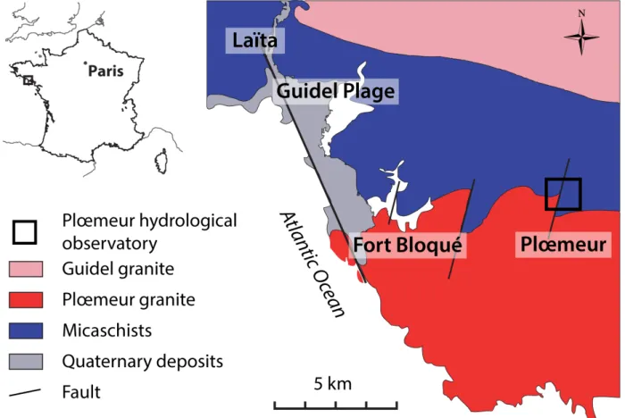
2009;Fabien-Ouellet and Fortier 2014;Pasquet et al. 2015). The use of this method is widespread

32

since it is easily carried out with a one-dimensional (1D) to three-dimensional (3D) coverage, quick

33

to implement and relatively inexpensive (Galibert et al. 2014). However, if measurements of VP

34

are performed quite efficiently for many years, retrieving VS remains complex since it requires the

35

use of horizontal component geophones difficult to set up horizontally (Sambuelli et al. 2001) and

36

specific sources strenuous to use (Sheriff and Geldart 1995; Jongmans and Demanet 1993; Xia et al.

37

2002;Haines 2007).

38

As an alternative to SH-wave refraction tomography, surface-wave prospecting methods are

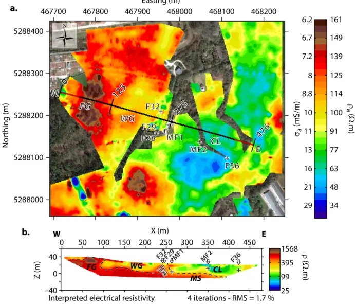
39

commonly proposed to achieve indirect estimation of VS in a relatively straightforward manner

40

(e.g.,Gabriels, Snieder, and Nolet(1987); Jongmans and Demanet (1993); Park, Miller, and Xia

41

(1999); Socco and Strobbia(2004); andSocco, Foti, and Boiero (2010a)). Due to their dispersive

42

nature, surface waves are characterized by an investigation depth that mainly depends on the

43

considered data frequency. Surface waves are thus widely used at large scales in global seismology for

44

mantle investigations using low frequencies. When targeting shallow structures with strong lateral

45

variability, surface-wave methods are, however, limited by the well-known trade-off between lateral

46

resolution and investigation depth (Gabriels et al. 1987). On the one hand, the inverse problem

47

formulation requires the investigated medium to be assumed 1D below the spread, which has to be

48

short enough to achieve lateral resolution and perform two-dimensional (2D) profiling. On the other

49

hand, long spreads and low-frequency geophones are required to record long wavelengths in order

50

to increase the investigation depth and mitigate near-field effects (Russel 1987;Forbriger 2003a,b;

51

O’Neill 2003;O’Neill and Matsuoka 2005;Bodet et al. 2005;Zywicki and Rix 2005;Bodet, Abraham,

52

and Clorennec 2009). When the seismic set-up provides redundant data, several countermeasures

53

exist to overcome these drawbacks and narrow down the lateral extent of dispersion measurements,

54

such as common mid-point cross-correlation (Hayashi and Suzuki 2004;Grandjean and Bitri 2006;

55

Ikeda, Tsuji, and Matsuoka 2013), multi-offset phase analysis (Strobbia and Foti 2006; Vignoli and

56

Cassiani 2010), or offset moving windows and dispersion stacking techniques (O’Neill, Dentith, and

57

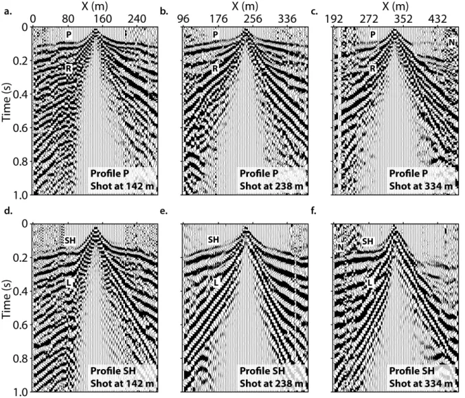
List 2003;Bohlen et al. 2004;Neducza 2007;Boiero and Socco 2010,2011;Bergamo, Boiero, and

58

Socco 2012).

59

The joint analysis of travel-time tomography VP and surface-wave profiling VS has recently

been proposed to retrieve 1D time-lapse VP/VS soundings (Pasquet et al. 2015) or 2D VP/VS

61

sections (Ivanov et al. 2006;Konstantaki et al. 2013).Pasquet et al.(2015) highlighted an overall

62

consistency between the temporal variations of the water table and VP/VS contrasts. For their

63

part, Konstantaki et al. (2013) assessed the lateral fluctuations of a shallow aquifer water table

64

level with 2D VP/VS variations. Using a single standard acquisition set-up to retrieve 2D VP and

65

VS sections thus appears interesting and convenient to reduce equipment costs and acquisition

66

time. Yet, refraction tomography and surface-wave profiling involve distinct characteristics of the

67

wavefield and different assumptions about the medium, thus providing results of different resolutions

68

and investigation depths difficult to compare to each other.

69

This study tackles such issues through a systematic comparison of VS models obtained from

70

SH-wave refraction and surface-wave dispersion inversion, along with VP retrieved from P-wave

71

refraction, as recently proposed by Pasquet et al. (2014, 2015). For this purpose, we targeted

72

the Plœmeur hydrological observatory (France). This experimental site has been subject to many

73

geophysical and hydrogeological studies aimed at characterizing the flow processes involved in the

74

recharge of the outstandingly productive fractured aquifer present in the region (Touchard 1999;

75

Le Borgne et al. 2006a,b, 2007; Ruelleu et al. 2010; Jim´enez-Mart´ınez et al. 2013). The study

76

area is located at a contact between granites and micaschists, clearly highlighted in the surface by

77

electrical resistivity tomography (ERT) and electrical conductivity (EC) mapping. However, previous

78

refraction seismic studies showed that VP alone was neither able to detect the contact zone nor able

79

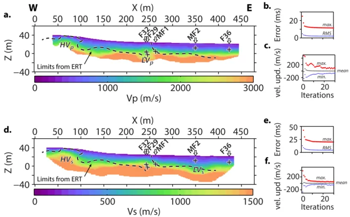
to discriminate granites from micaschists, probably because P-wave velocity is mainly controlled by

80

the water content in the weathered areas. The site consequently provided a challenging framework

81

to test the applicability of the joint interpretation of VP and VS for near-surface applications.

82

In the present study, VP and VS sections were classically obtained with P- and SH-wave

travel-83

time tomography carried out on a line intersecting the contact zone. Surface-wave profiling was

84

performed by means of offset moving window and dispersion stacking techniques. Local dispersion

85

measurements were first extracted from different shots illuminating the same portion of the seismic

86

line and then stacked to increase signal-to-noise ratio. The extraction window was eventually moved

87

along the line to retrieve a collection of local multimodal dispersion measurements. Several window

88

lengths were tested to find the best compromise between lateral resolution and investigation depth

89

(Pasquet et al. 2012). The lateral consistency of dispersion data was thoroughly controlled during

picking through visual browsing and a posteriori verified on phase velocity pseudo-sections. Separate

91

Monte Carlo inversions of dispersion curves were then performed along the line with no lateral

92

constraints in order to reconstruct a pseudo-2D VS section. The parameterization of those inversions

93

was based on: (i) VP obtained from travel-time tomography; (ii) a priori geological knowledge;

94

and (iii) maximum wavelengths observed along the line. Theoretical dispersion curves were then

95

recomputed from both VS models along the line to control the inversion quality and the consistency

96

of these models. Finally, VP/VS obtained from both methods were compared to evaluate their ability

97

to image VP/VS variations and assess their practical limitations.

98

2. SITE DESCRIPTION AND DATA ACQUISITION

99

2.1. Geological setting

100

The Plœmeur site is located on the south coast of Brittany (west of France), 3 km far from the

101

Atlantic Ocean, near the city of Lorient (Fig. 1). The crystalline bedrock aquifer present in the area

102

is composed of tectonic units developed during the Hercynian orogeny and marked by numerous

103

synkinematic intrusions of upper Carboniferous leucogranites (Ruelleu et al. 2010). The pumping

104

site is located at the intersection of: (i) a contact between the Plœmeur granite and overlying

105

“Pouldu” micaschists dipping 30◦ to the North and (ii) a subvertical fault zone striking N 20◦ (Fig.1).

106

Weathering in the area is limited to the first few metres, except in the micaschists near the pumping

107

site where it reaches about 30 m. Before the start of the pumping activities in 1991, the site was a

108

natural aquifer discharge area with preferential upward fluxes. The average water levels began to

109

decline during the first years of operation but have stabilized since 1997 (Jim´enez-Mart´ınez et al.

110

2013). Despite the low permeability and porosity of these lithologies, pumping wells implanted in

111

the site have been continuously producing water at a rate of about 106 m3 per year since 1991

112

(Touchard 1999), with limited head decrease and no seawater intrusion. One of the challenges on

113

this site is to understand recharge processes in these highly heterogeneous systems. For this purpose,

114

the site is monitored by several wells implanted mostly around the contact zone and in the clayey

115

area overlaying micaschists (F* and MF* in Fig. 2).

116

2.2. Previous geophysical results

117

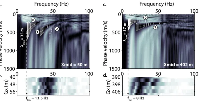
Slingram EC mapping and ERT were carried out on the site prior to the seismic campaign in

118

order to accurately describe near-surface lithologies. Apparent EC (σa) variations over the first

5.5 m in depth were mapped using an electromagnetic device with low induction number (intercoil

120

spacing of 3.66 m and frequency of 9.8 kHz) in vertical dipole (VD) configuration, integrating

121

conductivity values down to about 6 m in depth (McNeill 1980). We used a continuous acquisition

122

mode following profiles separated with 5 m to 7 m, covering an area of about 15 ha (Fig.2a). As for

123

ERT, we used a multi-channel resistivimeter with a 96-electrode Wenner–Schlumberger array and 1

124

roll-along (Fig. 2b). The electrodes were spaced with 4 m in order to obtain a 476-m-long profile

125

roughly oriented west–east (WE on Fig.2a). The inversion was performed using the RES2DINV

126

software (Loke and Barker 1996).

127

Results of EC mapping show smooth lateral variations of σa (from less than 5 mS/m to over

128

30 mS/m, i.e., from 200 Ωm to less than 30 Ωm in terms of apparent electrical resistivity ρa) in

129

the subsurface. Western low σa values are clearly associated with the presence of very shallow

130

granite (between 0 m and 125 m along the WE profile in Fig.2a). On the contrary, higher σa values

131

observed in the eastern part can be related to clays overlaying weathered micaschists (between 275 m

132

and 476 m in Fig.2a). Such distribution seems in agreement with the assumption of the contact

133

zone striking N 20◦ in the area. ERT results are also consistent with the anticipated geological

134

structures in depth and clearly match the apparent EC variations in surface (Fig.2b). Four main

135

structures can be delineated in Fig.2b: fresh granite (FG), almost outcropping in the western part,

136

characterized by high-electrical-resistivity (ρ) values (around 1000 Ωm); weathered granite (WG),

137

at the surface in the western part, characterized by significantly lower ρ values (around 200 Ωm);

138

clays (CL), at the surface in the eastern part, characterized by slightly lower ρ values (between

139

50 Ωm and 200 Ωm); and micaschists (MS), deeper in the eastern part, characterized by higher ρ

140

values (around 750 Ωm). Possible evidence of the contact zone is visible between 225 m and 250 m

141

along the ERT profile, marking a strong contrast between WG and clays (hashed area in Fig.2b).

142

The positions of the nearest piezometric wells are projected on the WE line with their measured

143

piezometric head level. A significant decrease in this level is observed in the wells located in the

144

hashed area due to pumping occurring in the F28 well. WhilePasquet et al. (2015) studied VP/VS

145

in simplified 1D conditions, this site offers the perfect framework to address 2D issues (i.e., presence

146

of strong lateral variations of lithology and topography), especially when knowing that previous

147

P-wave tomography studies failed to depict these lateral variations.

2.3. Seismic acquisition

149

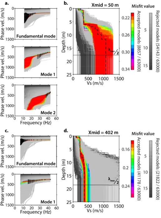
The seismic acquisition set-up was deployed along the ERT profile (WE in Fig.2a). It consisted

150

of a simultaneous P- and surface-wave acquisition followed by an SH-wave acquisition along the same

151

line. We used 72 geophones, a 4-m receiver spacing and 2 roll-alongs to finally obtain a 476-m-long

152

profile (Fig.3). A 72-channel seismic recorder was used with 14-Hz vertical component geophones

153

for the P-wave and surface-wave profiles and with 14-Hz horizontal component geophones for the

154

SH-wave profile. The use of 14-Hz geophones offers a good compromise to obtain seismic records

155

with a frequency content suitable for surface-wave, refraction, and reflection processing. First shot

156

location was one-half receiver spacing away from the first trace, and move-up between shots was one

157

receiver interval in order to achieve the high coverage required to perform refraction tomography

158

and to stack dispersion data. In addition, 219 shots were recorded along each profile for a total

159

number of 15768 active traces. The P-wave source consisted of an aluminium plate hit vertically by

160

a 5-kg sledgehammer. The plate was hit six times at each position to increase signal-to-noise ratio.

161

SH waves were generated with a handheld source consisting of a heavy metal frame hit laterally

162

by a 5-kg sledgehammer. The SH-wave source was hit 12 times at each position. For both P- and

163

SH-wave acquisitions, the sampling rate was 0.25 ms and the recording time was 2 seconds to

164

include full surface-wave wavefield. A delay of −0.02 seconds was kept before the beginning of each

165

record to prevent early triggering issues. The collected data presented on Fig.4 are affected with a

166

significant noise level, especially at far offset (80 m and more), due to active pumping wells and

167

military airplanes regularly landing and taking off from a nearby air force base. Seismograms clearly

168

show lateral variations due to both topographic effects and subsurface velocity changes, with strong

169

attenuation over clays and micaschists in the eastern part of the line.

170

3. TRAVEL-TIME TOMOGRAPHY

171

3.1. Travel-time data

172

We applied DC removal and a zero-phase low-pass filter on both P- and SH-wave data to remove

173

high-frequency noise (>100 Hz) and help for first arrival identification at far offsets. For the P-wave

174

profile, a total of 7076 first arrivals (45% of all traces) were determined (Fig.5a) and 10352 traces

175

(65% of all traces) were picked on SH-wave shots (Fig. 5c). Travel-time data could not be obtained

176

where noise level was too high (grey dots in Fig.5), with average maximum offsets around 100 m

for P waves and around 150 m for SH waves. Travel times are represented in a source–receiver

178

diagram (Fig. 5), which shows the distribution of first arrival times for each source–receiver pair

179

(Bauer et al. 2010;Baumann-Wilke et al. 2012). The diagonal traces indicate the zero-offset travel

180

times, where source and receiver locations are identical. This representation gives a first impression

181

of the subsurface velocity structure and allows for checking the lateral consistency of picked travel

182

times. Three main areas are clearly visible on both P- and SH-wave first arrivals: the first area

183

(from 0 m to 125 m) is characterized by the shortest first arrival times (i.e., shallow high velocity

184

zone); the area between 125 m and 275 m depicts slightly increasing times; and the third area

185

(from 275 m up to the end of the line) shows greater arrival times (compared with the first area),

186

probably associated with shallow low velocities.

187

The distribution depicted in Fig.5a and5c appears interestingly related to the lateral variability

188

observed on the EC map (Fig.2a). Along the seismic profile, very low σa values occur between

189

0 m and 125 m on the granite side and are coherent with short first arrival times. High-σa values

190

observed between 275 m and the end of the line are also consistent with the shallow low velocity

191

zone suggested by long first arrival times. In the centre part (from 125 m to 275 m), intermediate

192

apparent EC values are in agreement with slightly decreasing shallow velocities observed in Fig.5a

193

and 5c, suggesting a thickening of the weathered layer.

194

3.2. Tomography inversion

195

Travel-time data were inverted with the refraction tomography software RAYFRACT (Schuster

196

and Quintus-Bosz 1993;Sheehan, Doll, and Mandell 2005;Rohdewald 2011) using a smooth gradient

197

initial model. This model is the 2D extension of the mean 1D model obtained directly from picked

198

travel times, assuming velocity gradients in a 1D tabular medium (Gibson, Odegard, and Sutton

199

1979). It varied from 10 m/s at the surface to 3500 m/s at 40 m in depth for the P-wave model and

200

from 10 m/s at the surface to 2000 m/s at 40 m in depth for the SH-wave model. The inversion

201

process was stopped when velocity update, global root-mean-square (RMS) error, and maximum

202

normalized residual reached minimum values. In addition, 30 iterations were needed for both

P-203

and SH-wave travel times. For the P-wave profile, the global RMS error (in blue in Fig.6b) and the

204

maximum normalized residual (in red in Fig.6b) both steeply decrease during the first six iterations,

205

i.e., from 5 ms to 2.5 ms and from 25 ms to 13 ms, respectively, and more gradually during the last

206

iteration steps until they both reach minimum values of 2.1 ms and 11.5 ms, respectively. Mean

velocity update also rapidly decreases to reach a minimum value after six iterations (in black in

208

Fig. 6c). Maximum and minimum velocity updates (in red and blue, respectively, in Fig.6c) are

209

more perturbated and tend to stabilize only after 20 iterations. As for SH-wave data, the global

210

RMS error (in blue in Fig. 6e) and the maximum normalized residual (in red in Fig. 6e) both

211

quickly decrease during the first 10 iterations, i.e., from 12.5 ms to 6 ms and from 50 ms to 22 ms,

212

respectively, and more smoothly during the last iteration steps until they both reach minimum

213

values of 4.3 ms and 20.1 ms, respectively. Mean, maximum, and minimum velocity updates (in

214

black, red, and blue, respectively, in Fig. 6f) reach minimum values after 10 iterations.

215

Normalized residuals were computed between observed and calculated travel times for every

216

picked trace (Bauer et al. 2010). Their distributions are represented in source–receiver diagrams for

217

both P- (Fig.5b) and SH-wave (Fig.5d) travel times. P-wave inversion results have lower global

218

RMS values (2.1 ms for P waves; 4.3 ms for SH waves) and maximum residual values (11.5 ms for

219

P waves; 20.1 ms for SH waves), and the mean residual value is higher for P waves (6.7%) than for

220

SH waves (3.9%). The ratio of residuals below 10% is also higher for SH-wave models (around 93%)

221

than for P-wave models (around 91%). The distribution of residuals shows the highest values at near

222

offsets, probably due to shallow lateral heterogeneities and triggering issues during the acquisition.

223

The final velocity models were clipped for both VP (Fig. 6a) and VS (Fig.6d) sections below a

224

ray coverage of 100 rays per grid cell to keep only well-resolved areas. Both models are characterized

225

by velocities mainly following a linearly increasing trend in depth and show no strong lateral

226

variations. Only slight perturbations of the initial gradient model along the line can be observed

227

with: (i) higher VP and VS in the western part (HVP and HVS, respectively), corresponding to the

228

high-electrical-resistivity values associated with FG; (ii) lower VP in the centre (LVP), consistent

229

with a decrease in the piezometric head level and evidences of the contact zone inferred from ERT;

230

and (iii) lower VS in the eastern part of the profile (LVS).

231

4. SURFACE-WAVE PROFILING

232

4.1. Extraction of dispersion curves

233

Our multifold acquisition set-up allowed us to obtain surface-wave dispersion images from

234

P-wave shot gathers using windowing and dispersion stacking to narrow down the lateral extent of

235

dispersion measurements and increase the signal-to-noise ratio. Dispersion stacking was performed

following the basic workflow derived from O’Neill et al.(2003).

237

1. Select nW traces centred on a specific position along the line (Xmid).

238

2. Load a shot illuminating the selected spread.

239

3. Window the nW traces in the selected shot record.

240

4. Transform the wavefield to the frequency-phase velocity domain (dispersion image).

241

5. Normalize amplitude spectrum at each frequency.

242

6. Repeat steps 2–5 for the nS selected shots.

243

7. Stack all normalized dispersion images and pick the dispersion curves for each identified

propa-244

gation mode from the final image.

245

8. Shift the window of dW traces to the next Xmid and repeat steps 1–7.

246

As aforementioned, the difficulty is to find the best compromise between investigation depth,

247

spectral resolution, and lateral resolution while keeping the 1D assumption valid. Thus, we first

248

performed trial-and-error tests (Pasquet et al. 2012) to select the optimum window size (nW )

249

and the number of sources (nS), keeping in mind that there is not, for the moment, any perfect

250

criterion (P´erez Solano 2013;P´erez Solano, Donno, and Chauris 2014). A 20-m-wide window with

251

six traces (nW = 6) was eventually used with six direct and six reverse shots on each side of the

252

window (nS = 6). Using more sources is likely to increase signal-to-noise ratio and enhance the

253

maxima but would narrow down the effective study area along the line (black dots in Fig. 2a).

254

Single dispersion images were obtained from each shot using a slant stack in the frequency domain

255

(Russel 1987; Mokhtar, Herrmann, and Russell 1988). These images (in which maxima should

256

correspond to Rayleigh-wave propagation modes) were first compared to confirm the validity of

257

the 1D approximation below the spread (Jongmans et al. 2009). These 12 single dispersion images

258

were then stacked as a final dispersion image. The moving window was finally shifted along the line

259

with a step of one receiver spacing (dW = 1, i.e., 4 m). We thus obtained evenly spaced dispersion

260

images at each spread mid-point (Xmid) with a large overlap in order to retrieve smoothly varying

261

dispersion images between two adjacent stacking windows and help for visual browsing when picking

262

dispersion curves.

263

We eventually obtained a collection of 105 stacked dispersion images along the line, on which

264

coherent maxima associated with the different propagation modes were identified. Visualization

265

of adjacent stacked dispersion images allowed for following the progressive lateral evolution of

the different modes and for avoiding mode misinterpretation (Zhang and Chan 2003;O’Neill and

267

Matsuoka 2005;Boaga et al. 2013;Ezersky et al. 2013). These maxima were finally extracted on

268

each stacked dispersion image with an estimated standard error in phase velocity defined according

269

to the workflow described inO’Neill (2003). The dispersion lateral variability is illustrated here

270

by two examples at both sides of the line (Fig. 7a (Xmid = 50 m) and 7c (Xmid = 402 m)).

271

As, for instance, recommended by Bodet (2005) and Bodet et al. (2009), dispersion curves were

272

limited down to frequencies (flim) where the spectral amplitude of the seismogram became too low

273

(13.5 Hz in Fig.7b and 8 Hz in Fig.7d). Several authors (e.g., O’Neill(2003) and Zywicki and Rix

274

(2005)) also mentioned that wavelengths higher than 50% of the spread length should not be used

275

in order to mitigate near-field effects and prevent from velocity underestimation at low frequency.

276

These recommendations are only basic rules of thumb mostly valid when using the fundamental

277

mode only. Here, we used wavelengths higher than 50% of our spread length since we were able to

278

perform dispersion stacking and use higher modes, which are of great constraint on the inversion

279

with a strong impact on the investigation depth (Gabriels et al. 1987;Xia et al. 2003). Furthermore,

280

possible low-frequency discrepancies were limited by attributing important errors to dispersion data

281

with respect to frequency and spread length (O’Neill 2003). Finally, the corresponding maximum

282

wavelength (λmax) was extracted (35 m in Fig.7a and 37 m in Fig.7c) to retrieve λmax/2, a typical

283

investigation depth criterion (O’Neill 2003).

284

Up to four propagation modes were observed along the line and identified as fundamental (0),

285

first (1), second (2), and third (3) higher modes (only modes up to 2 were identified in the examples

286

shown in Fig. 7). The resulting dispersion curves are presented in Rayleigh-wave phase velocity

287

pseudo-sections as a function of the wavelength λ and the spread mid-point Xmid (Fig.8) in order

288

to control the lateral coherence of mode identification (Strobbia et al. 2011; Haney and Douma 2012;

289

Boiero et al. 2013a; Ezersky et al. 2013). The fundamental mode pseudo-section (Fig. 8a) does not

290

present unrealistic abrupt changes (considering the overlap between two adjacent stacking windows)

291

but shows significant lateral variations of Rayleigh-wave phase velocities. High phase velocities

292

(from 200 m/s to 550 m/s) exist in the western part of the line (from the beginning to around

293

100 m), whereas the eastern part of the line (from 275 m to the end) is characterized by lower

294

phase velocities (around 150 m/s–200 m/s). The first (Fig.8b), second (Fig.8c), and third (Fig.8d)

295

higher modes show less lateral variations in terms of velocity, but the available frequency range for

mode 1 presents significant lateral fluctuations. The maximum wavelength (λmax) observed at each

297

Xmid ranges from 20 m to 50 m with an average value around 30 m (Fig.8e).

298

4.2. Inversion

299

Assuming a 1D tabular medium below each extraction window, we performed a 1D inversion of

300

dispersion data obtained at each Xmid. We used the neighbourhood algorithm (NA) developed

301

by Sambridge(1999) and implemented for near-surface applications by Wathelet, Jongmans, and

302

Ohrnberger(2004) and Wathelet(2008) within the GEOPSY tool (available atwww.geopsy.org).

303

Theoretical dispersion curves were computed from the elastic parameters using the Thomson–Haskell

304

matrix propagator technique (Thomson 1950;Haskell 1953). NA performs a stochastic search of

305

a pre-defined parameter space (namely, VP, VS, density, and thickness of each layer) using the

306

following misfit function (MF ):

307 M F = v u u t Nf X i=1 (Vcali− Vobsi) 2 Nfσi2 , (1)

with Vcali and Vobsi being the the calculated and observed phase velocities at each frequency fi, Nf 308

being the number of frequency samples, and σi being the phase velocity measurement error at each

309

frequency fi.

310

An appropriate choice of these parameters is considered as a fundamental issue for the successful

311

application of inversion (Socco and Strobbia 2004; Renalier et al. 2010). Based on site a priori

312

geological knowledge (presence of weathering gradients), we used parameterization with a stack

313

of ten layers overlaying the half-space to look for a velocity gradient. The thickness of each layer

314

was allowed for ranging from 0.5 m to 2.5 m. The maximum half-space depth (HSD) is of great

315

importance since it depends on the poorly known investigation depth of the method. It was fixed to

316

the half of the maximum wavelength observed along the entire line (25 m), as recommended by

317

O’Neill (2003) andBodet et al. (2005). The valid parameter range for sampling velocity models

318

was 10 m/s–1500 m/s for VS (based on dispersion observations and refraction tomography), with

319

velocities constrained to only increase with depth, based on geological a priori information. P-wave

320

velocity being of weak constraint on surface-wave dispersion, only the S-wave velocity profile can be

321

interpreted (Der and Landisman 1972;Russel 1987). However, an identical layering is required for

322

VP and VS in order to interpret VP/VS ratios. For this purpose, we extracted an average VP value

for each 2.5-m-thick slice of the VP model obtained from refraction tomography (Fig. 6a). This

324

average value was then used to fix VP in each layer of the inversion parameterization. Furthermore,

325

VS values were allowed to vary in such a way that Poisson’s ratio values always remained between

326

0.1 and 0.5 in order to prevent from unrealistic VS values. Density was set as uniform (1800 kg/m3)

327

since its influence on dispersion curves is very limited (Der and Landisman 1972; Russel 1987). It is

328

worth mentioning that, except for the VP values, we used the same parameterization for all the 1D

329

inversions performed along the line. We assumed that stacking and windowing already naturally

330

smoothed the dispersion data, thus not requiring the use of lateral constraints between successive

331

inversions.

332

A total of 63000 models were generated with NA (Fig. 9a (Xmid = 50 m) and 9c (Xmid =

333

402 m)). Models matching the observed data within the error bars were selected, as suggested

334

byEndrun et al.(2008). The accepted models were used to build a final average velocity model

335

associated with the centre of the extraction window (dashed line in Fig.9b (Xmid = 50 m) and9d

336

(Xmid = 402 m)). As the maximum HSD remains constant along the line (same parameterization

337

for each inversion), λmax/2 is given (solid black line in Fig. 9b and 9d) to show where inverted

338

models expand below typical investigation depth criterion. Normalized residuals between observed

339

and calculated phase velocities were computed along the line for each individual sample of the picked

340

dispersion curves. Their distributions are represented in pseudo-sections to control the quality of

341

the final pseudo-2D VS section. The fundamental mode residuals’ pseudo-section (Fig.10a) shows

342

quite uniform values, with a maximum of 19%, a mean residual of 5%, and 86% of the residuals

343

with values below 10%. Residual values obtained for the first higher mode (Fig.10b) present higher

344

values, especially at great wavelength. The maximum residual value is 29%, the mean is 9%, and

345

only 62% of the residuals are below 10%. As for the second and the third higher modes (Fig.10c

346

and10d, respectively), residuals remain very low with a maximum of 12% and 3%, respectively, and

347

a mean residual of 1.8% and 1.3%, respectively. In addition, 99% of the second higher mode samples

348

have residual values below 10%, whereas all samples of the third higher mode have residuals below

349

10%. We additionally computed the misfit for each 1D VS model along the line with equation (1)

350

(Fig.10e). Misfit values remain stable along the line and range from 0.05 to around 0.25, with a

351

mean value of about 0.125. Several gaps are present along the line and correspond to inversions

352

where none of the calculated models were fitting the error bars.

Each 1D VS model was then represented at its corresponding Xmid position to obtain a

pseudo-354

2D VS section (Fig. 11). All the models were represented down to the maximum HSD (25 m),

355

with the investigation depth criterion λmax/2 superimposed in hashed black line. With such a

356

representation, the actual HSD of each model can be easily followed along the line and compared

357

with the investigation depth criterion. If the lateral variations of VS values remain remarkably

358

smooth in the shallow layers, the deepest layers and the half-space present an important variability

359

of VS caused by the higher uncertainties in dispersion measurements at great wavelength (i.e.,

360

higher residual values in Fig.10). Global results show a shallow low velocity layer (∼ 250 m/s),

361

which is thinner in the western part of the line (from 3 m to 6 m) and becomes thicker (∼ 10 m) in

362

the eastern part. High velocities (between 500 m/s and 1000 m/s) can be observed in the western

363

part, directly below the shallow low velocity layer, whereas the velocity of the half-space remains

364

below 500 m/s in the eastern part.

365

5. QUALITATIVE COMPARISON OF VELOCITY MODELS AND RESULTING

366

VP/VS

367

The comparison of velocity models obtained from P-wave tomography (V_Ptomo, Fig.6a), SH-wave

368

tomography (V_Stomo, Fig.6b), and surface-wave dispersion profiling (V_Ssw, Fig.11) provided results

369

that are consistent with the main structures interpreted from ERT data (Fig.2b). However, velocity

370

models do not provide such a clear delineation of these structures, especially for V_Ptomo and V_Stomo

371

sections. Indeed, the travel-time tomography method smoothes the lateral variations of velocity and

372

often suffers from the strong influence of triggering issues on short travel times, which mainly affect

373

the reconstruction of shallow structure velocities. As for surface-wave profiling, the overlaying of

374

structures delimited by ERT on the V_Ssw pseudo-2D section (Fig.11) confirms the lateral consistency

375

of both VS models in the first 20 m in depth. If the surface-wave method is clearly limited by its

376

low investigation depth in this case, it provides more information regarding the lateral variations of

377

shallow layers’ velocities and seems to detect the modifications of mechanical properties occurring

378

in the contact zone.

379

At both Xmid = 50 m (Fig. 12a) and Xmid = 402 m (Fig. 12d), 1D models of VS and VP

380

extracted from tomography sections (V_Stomo in green solid line and V_Ptomo in green dashed line,

381

respectively) are characterized by similar trends of continuously increasing velocities in depth.

Furthermore, 1D V_Ssw models (red solid line) show the presence of two constant velocity layers

383

followed by a linearly increasing velocity layer overlaying the half-space. Despite a low investigation

384

depth, the V_Ssw pseudo-section manages to depict the shallow lateral variations and remains in good

385

agreement with V_Stomo.

386

As a control of both VS models, forward modelling was performed along the line (examples

387

for Xmid = 50 m and Xmid = 402 m are shown in Fig. 12c and 12f, respectively). On the one

388

hand, theoretical dispersion curves were computed using 1D V_Ptomo and V_Stomo models (green solid

389

line). On the other hand, theoretical dispersion curves were calculated using 1D V_Ssw models and

390

1D V_Ptomo models resampled in depth according to the V_Ssw layering (V_Prs) (red solid line). V_Ssw

391

models provide the best fit with the picked dispersion curves and the coherent maxima observed on

392

dispersion images, supporting the validity of the final V_Ssw model averaged from all models fitting

393

the error bars. For their part, dispersion curves computed from V_Stomo models are generally not well

394

fitting the observed propagation modes at low frequency, leading us to question the validity of the

395

tomographic model in the deepest layers.

396

After cross-validating both VS models, we computed VP/VS ratios along the line with: (i) VSsw

397

and V_Prs (Fig. 13a) and (ii) V_Stomo and V_Ptomo (Fig.13b). The V_Stomo/V_Ptomo section shows smooth

398

lateral variations, with low VP/VS (∼ 1.5) in the western (from 0 m to 150 m) and central

399

(from 200 m to 250 m) parts, separated by intermediate values (∼ 2–2.5). The eastern part is

400

characterized by higher values (around 2.5 and up to 3.5). At first sight, the Vsw

S /VPrs section might

401

look different, especially in the beginning of the line (from 0 m to 275 m), where anomalous high

402

VP/VS values are observed around 5-m to 10-m depth. At these depths, the VSsw model presents

403

mostly constant velocities, whereas the V_Prs model is characterized by linearly increasing velocities.

404

This incompatibility can thus explain the VP/VS discrepancies observed in this layer. With this in

405

mind, we were yet able to delineate different VP/VS areas, which correspond well to those observed

406

on the Vtomo

S /VPtomosection. These different areas and the observed VP/VS values are also consistent

407

with the main structures delineated in the ERT results (Fig. 2b), whereas it was not clear on VP or

408

VS only.

409

Moreover, 1D VP/VS ratios extracted at Xmid = 50 m (Fig.12b) and Xmid = 402 m (Fig.12e)

410

from V_Prs/V_Ssw (red solid line) and V_Ptomo/V_Stomo (green solid line) show similar trends. Stronger

411

contrasts and higher ratio values are yet observed on surface-wave analysis results. VP/VS values

observed at Xmid = 50 m are overall low (below 2.75) with both methods. The water table level

413

extrapolated from the nearest representative piezometric well implanted in the granite (around

414

100 m west from Xmid = 50 m) is not consistent with any of the contrasts observed on the VP/VS

415

models. Indeed, the estimated water table level (∼ 20 m) is close to the maximum HSD where

416

V_Ssw becomes poorly resolved. Furthermore, no strong VP/VS variations can be anticipated in

417

such low-permeability and low-porosity materials (Takei 2002). At Xmid = 402 m, shallow high

418

VP/VS ratio values (around 4) are consistent with a wet soil, whereas a strong contrast at 11.5-m

419

depth remarkably matches the water table level interpolated from levels measured in MF2 and F36

420

(black dashed line). This feature is confirmed on the pseudo-2D VP/VS section in the eastern part

421

(Fig. 13a).

422

6. DISCUSSION AND CONCLUSIONS

423

In order to assess the applicability of combined P-wave refraction tomography and surface-wave

424

dispersion analysis to estimate VP/VS ratio in near-surface applications, we performed seismic

425

measurements on a well-known granite–micaschists contact at Plœmeur hydrological observatory

426

(France). A simultaneous P- and surface-wave survey was achieved using a single acquisition set-up

427

and was supplemented with an SH-wave acquisition along the same line in order to compare VS

428

results obtained from SH-wave refraction tomography and surface-wave profiling.

429

P- and SH-wave first arrivals observed along the line were used to perform travel-time tomography

430

and retrieve V_Ptomo and V_Stomo models. Evenly spaced dispersion data were extracted along the line

431

from P-wave shot gathers using windowing and stacking techniques. Successive 1D Monte Carlo

432

inversions of these dispersion data were achieved using fixed VP values extracted from the V_Ptomo

433

model and no lateral constraints between two adjacent 1D inversions. The resulting 1D V_Ssw models

434

were then assembled to create a pseudo-2D V_Ssw section. We computed normalized residuals between

435

observed and calculated phase velocities along the line to control the quality of the V_Ssw model.

436

This model appears to be correctly matching the V_Stomo model obtained with SH-wave refraction

437

tomography. The V_Ssw model is however characterized by strong velocity uncertainties in the deepest

438

layers. The recomputation of theoretical dispersion curves along the line also provided results that

439

are consistent with the measured dispersion images and proved to be a reliable tool for validating

440

VS models obtained from SH-wave refraction tomography and surface-wave profiling. Finally, we

were able to compute VP/VS sections from both V_Ssw and V_Stomo. The two sections present similar

442

features, but the section obtained from V_Ssw shows a higher lateral resolution, which is consistent

443

with the features observed on ERT, thus validating our approach for retrieving VP/VS ratio from

444

combined P-wave tomography and surface-wave profiling. Furthermore, the VP/VS ratios obtained

445

in the clay and micaschists area show a strong contrast consistent with the observed water table

446

level.

447

An incompatibility, however, remains between V_Prsand V_Ssw, which can lead to anomalous VP/VS

448

values. Indeed, travel-time tomography provides a smooth 2D reconstruction of the medium along

449

ray paths propagating from sources to sensors in a narrow frequency band. The investigation depth

450

is strongly related to the length of the acquisition profile and the maximum offset between sources

451

and receivers. Furthermore, the medium is described as a function of the ray coverage, which is

452

strongly related to the spacing between sensors and usually increases in high-velocity zones. For

453

their part, surface-wave methods allow reconstructing pseudo-2D VS sections by juxtaposing single

454

1D models obtained along the line. In this case, the spectral resolution and the investigation depth

455

are a function of the frequency and increase with the length of the recording array, whereas the

456

lateral resolution is inversely correlated with the individual array length. In order to retrieve VP and

457

VS models more suited for VP/VS computation, a joint inversion approach combining Rayleigh and

458

P-guided waves dispersion data along with P-wave refraction travel times could be developed, in

459

the continuation ofMaraschini et al. (2010),Piatti et al. (2013) andBoiero, Wiarda, and Vermeer

460

(2013b) works.

461

7. ACKNOWLEDGEMENTS

462

The authors would like to thank Claudio Strobbia, Daniela Donno, and two anonymous reviewers

463

for their constructive comments. This work was supported by the French National Programme

464

EC2CO – Biohefect (Project “ ´Etudes exp´erimentales multi-´echelles de l’apport des vitesses sismiques

465

`

a la description du continuum sol-aquif`ere”) and the ANR Project CRITEX ANR-11-EQPX-0011. It

466

was also supported by the SOERE-H+ “R´eseau National de sites hydrog´eologiques” network and by

467

the CLIMAWAT European Project “Adapting to the Impacts of Climate Change on Groundwater

468

Quantity and Quality”. They kindly thank A. Kehil, J. Jimenez-Martinez, E. Coulon, and N.

469

Lavenant (G´eosciences Rennes) for technical assistance during field work. They would also like to

thank J. Thiesson (UMR METIS) for valuable discussions during data processing and interpretation.

8. REFERENCES

472

Bauer K., Moeck I., Norden B., Schulze A., Weber M. and Wirth H. 2010. Tomographic P wave velocity and

473

vertical velocity gradient structure across the geothermal site Groß Sch¨onebeck (NE German Basin): relationship

474

to lithology, salt tectonics, and thermal regime. Journal of Geophysical Research: Solid Earth 115(B8), B08312.

475

Bauer K., Schulze A., Ryberg T., Sobolev S.V. and Weber M.H. 2003. Classification of lithology from seismic

476

tomography: a case study from the Messum igneous complex, Namibia. Journal of Geophysical Research: Solid

477

Earth 108(B3), 2152.

478

Baumann-Wilke M., Bauer K., Schovsbo N.H. and Stiller M. 2012. P-wave traveltime tomography for a seismic

479

characterization of black shales at shallow depth on Bornholm, Denmark. Geophysics 77(5), EN53–EN60.

480

Bergamo P., Boiero D. and Socco L.V. 2012.Retrieving 2D structures from surface-wave data by means of space-varying

481

spatial windowing. Geophysics 77(4), EN39–EN51.

482

Berryman J.G. 1999. Origin of Gassmann’s equations. Geophysics 64(5), 1627–1629.

483

Biot M.A. 1956a. Theory of propagation of elastic waves in a fluid-saturated porous solid. I. Low-frequency range.

484

The Journal of the Acoustical Society of America 28(2), 168–178.

485

Biot M.A. 1956b. Theory of propagation of elastic waves in a fluid-saturated porous solid. II. Higher frequency range.

486

The Journal of the Acoustical Society of America 28(2), 179–191.

487

Boaga J., Cassiani G., Strobbia C. and Vignoli G. 2013. Mode misidentification in Rayleigh waves: ellipticity as a

488

cause and a cure. Geophysics 78(4), EN17–EN28.

489

Bodet L. 2005. Limites th´eoriques et exp´erimentales de l’interpr´etation de la dispersion des ondes de Rayleigh: apport

490

de la mod´elisation num´erique et physique. PhD thesis, ´Ecole Centrale de Nantes et Universit´e de Nantes, France.

491

Bodet L., Abraham O. and Clorennec D. 2009.Near-offset effects on Rayleigh-wave dispersion measurements: physical

492

modeling. Journal of Applied Geophysics 68(1), 95–103.

493

Bodet L., van Wijk K., Bitri A., Abraham O., Cˆote P., Grandjean G. et al. 2005. Surface-wave inversion limitations

494

from laser-Doppler physical modeling. Journal of Environmental and Engineering Geophysics 10(2), 151–162.

495

Bohlen T., Kugler S., Klein G. and Theilen F. 2004. 1.5D inversion of lateral variation of Scholte-wave dispersion.

496

Geophysics 69(2), 330–344.

497

Boiero D. and Socco L.V. 2010. Retrieving lateral variations from surface wave dispersion curves. Geophysical

498

Prospecting 58(6), 977–996.

499

Boiero D. and Socco L.V. 2011. The meaning of surface wave dispersion curves in weakly laterally varying structures.

500

Near Surface Geophysics 9(6), 561–570.

501

Boiero D., Socco L.V., Stocco S. and Wis´en R. 2013a. Bedrock mapping in shallow environments using surface-wave

502

analysis. The Leading Edge 32(6), 664–672.

503

Boiero D., Wiarda E. and Vermeer P. 2013b. Surface- and guided-wave inversion for near-surface modeling in land

504

and shallow marine seismic data. The Leading Edge 32(6), 638–646.

505

Cardarelli E., Cercato M. and De Donno G. 2014. Characterization of an earth-filled dam through the combined use

506

of electrical resistivity tomography, P- and SH-wave seismic tomography and surface wave data. Journal of Applied

507

Geophysics 106, 87–95.

Catchings R.D. 1999. Regional Vp, Vs, Vp/Vs, and Poisson’s ratios across earthquake source zones from Memphis,

509

Tennessee, to St. Louis, Missouri. Bulletin of the Seismological Society of America 89(6), 1591–1605.

510

Der Z.A. and Landisman M. 1972. Theory for errors, resolution, and separation of unknown variables in inverse

511

problems, with application to the mantle and the crust in southern Africa and Scandinavia. Geophysical Journal of

512

the Royal Astronomical Society 27(2), 137–178.

513

Dvorkin J. 2008. Yet another Vs equation. Geophysics 73(2), E35–E39.

514

Endrun B., Meier T., Lebedev S., Bohnhoff M., Stavrakakis G. and Harjes H.P. 2008. S velocity structure and radial

515

anisotropy in the Aegean region from surface wave dispersion. Geophysical Journal International 174(2), 593–616.

516

Ezersky M.G., Bodet L., Akawwi E., Al-Zoubi A.S., Camerlynck C., Dhemaied A. et al. 2013. Seismic surface-wave

517

prospecting methods for sinkhole hazard assessment along the Dead Sea shoreline. Journal of Environmental and

518

Engineering Geophysics 18(4), 233–253.

519

Fabien-Ouellet G. and Fortier R. 2014. Using all seismic arrivals in shallow seismic investigations. Journal of Applied

520

Geophysics 103, 31–42.

521

Forbriger T. 2003a. Inversion of shallow-seismic wavefields: I. Wavefield transformation. Geophysical Journal

522

International 153(3), 719–734.

523

Forbriger T. 2003b.Inversion of shallow-seismic wavefields: II. Inferring subsurface properties from wavefield transforms.

524

Geophysical Journal International 153(3), 735–752.

525

Fu D.T., Sullivan E.C. and Marfurt K.J. 2006. Rock-property and seismic-attribute analysis of a chert reservoir in

526

the Devonian Thirty-one Formation, west Texas, U.S.A. Geophysics 71(5), B151–B158.

527

Gabriels P., Snieder R. and Nolet G. 1987.In situ measurements of shear-wave velocity in sediments with higher-mode

528

Rayleigh waves. Geophysical Prospecting 35(2), 187–196.

529

Galibert P.Y., Valois R., Mendes M. and Gu´erin R. 2014.Seismic study of the low-permeability volume in southern

530

France karst systems. Geophysics 79(1), EN1–EN13.

531

Gautier S., Latorre D., Virieux J., Deschamps A., Skarpelos C., Sotiriou A. et al. 2006. A new passive tomography of

532

the Aigion area (Gulf of Corinth, Greece) from the 2002 data set. Pure and Applied Geophysics 163(2–3), 431–453.

533

Gibson B.S., Odegard M.E. and Sutton G.H. 1979. Nonlinear least-squares inversion of traveltime data for a linear

534

velocity-depth relationship. Geophysics 44(2), 185–194.

535

Godio A., Strobbia C. and De Bacco G. 2006. Geophysical characterisation of a rockslide in an alpine region.

536

Engineering Geology 83(1–3), 273–286.

537

Grandjean G. and Bitri A. 2006. 2M-SASW : Multifold multichannel seismic inversion of local dispersion of Rayleigh

538

waves in laterally heterogeneous subsurfaces: application to the Super-Sauze earthflow, France. Near Surface

539

Geophysics 4(6), 367–375.

540

Grelle G. and Guadagno F.M. 2009. Seismic refraction methodology for groundwater level determination: “Water

541

seismic index”. Journal of Applied Geophysics 68(3), 301–320.

542

Haines S. 2007. A hammer-impact, aluminium, shear-wave seismic source. Technical Report OF 07-1406. United

543

States Geological Survey.

544

Haney M.M. and Douma H. 2012. Rayleigh-wave tomography at Coronation Field, Canada: The topography effect.

545

The Leading Edge 31(1), 54–61.

Haskell N.A. 1953.The dispersion of surface waves on multilayered media. Bulletin of the Seismological Society of

547

America 43(1), 17–34.

548

Hayashi K. and Suzuki H. 2004. CMP cross-correlation analysis of multi-channel surface-wave data. Exploration

549

Geophysics 35(1), 7–13.

550

Heitor A., Indraratna B., Rujikiatkamjorn C. and Golaszewski R. 2012. Characterising compacted fills at Penrith

551

Lakes development site using shear wave velocity and matric suction. In: 11th Australia - New Zealand Conference

552

on Geomechanics: Ground Engineering in a Changing World, Melbourne, Australia. pp. 1262–1267.

553

Hibert C., Grandjean G., Bitri A., Travelletti J. and Malet J.P. 2012. Characterizing landslides through geophysical

554

data fusion: Example of the La Valette landslide (France). Engineering Geology 128, 23–29.

555

Ikeda T., Tsuji T. and Matsuoka T. 2013. Window-controlled CMP crosscorrelation analysis for surface waves in

556

laterally heterogeneous media. Geophysics 78(6), EN95–EN105.

557

Ivanov J., Miller R.D., Xia J., Steeples D. and Park C.B. 2006. Joint analysis of refractions with surface waves: an

558

inverse solution to the refraction-traveltime problem. Geophysics 71(6), R131–R138.

559

Jim´enez-Mart´ınez J., Longuevergne L., Le Borgne T., Davy P., Russian A. and Bour O. 2013. Temporal and spatial

560

scaling of hydraulic response to recharge in fractured aquifers: Insights from a frequency domain analysis. Water

561

Resources Research 49(5), 3007–3023.

562

Jongmans D. 1992.The application of seismic methods for dynamic characterization of soils in earthquake engineering.

563

Bulletin of the International Association of Engineering Geology - Bulletin de l’Association Internationale de

564

G´eologie de l’Ing´enieur 46(1), 63–69.

565

Jongmans D., Bi`evre G., Renalier F., Schwartz S., Beaurez N. and Orengo Y. 2009. Geophysical investigation of a

566

large landslide in glaciolacustrine clays in the Tri`eves area (French Alps). Engineering Geology 109(1–2), 45–56.

567

Jongmans D. and Demanet D. 1993. The importance of surface waves in vibration study and the use of Rayleigh

568

waves for estimating the dynamic characteristics of soils. Engineering Geology 34(1–2), 105–113.

569

Juli`a J. and Mej´ıa J. 2004.Thickness and Vp/Vs ratio variation in the Iberian crust. Geophysical Journal International

570

156(1), 59–72.

571

Konstantaki L., Carpentier S., Garofalo F., Bergamo P. and Socco L.V. 2013. Determining hydrological and soil

572

mechanical parameters from multichannel surface-wave analysis across the Alpine Fault at Inchbonnie, New Zealand.

573

Near Surface Geophysics 11(4), 435–448.

574

Lai C.G. and Rix G.J. 1998. Simultaneous inversion of Rayleigh phase velocity and attenuation for near-surface site

575

characterization. Report No. GIT-CEE/GEO-98-2. Georgia Institute of Technology.

576

Latorre D., Virieux J., Monfret T., Monteiller V., Vanorio T., Got J.L. et al. 2004. A new seismic tomography of

577

Aigion area (Gulf of Corinth, Greece) from the 1991 data set. Geophysical Journal International 159(3), 1013–1031.

578

Le Borgne T., Bour O., Paillet F.L. and Caudal J.P. 2006a. Assessment of preferential flow path connectivity and

579

hydraulic properties at single-borehole and cross-borehole scales in a fractured aquifer. Journal of Hydrology

580

328(1–2), 347–359.

581

Le Borgne T., Bour O., Riley M.S., Gouze P., Pezard P.A., Belghoul A. et al. 2007. Comparison of alternative

582

methodologies for identifying and characterizing preferential flow paths in heterogeneous aquifers. Journal of

583

Hydrology 345(3–4), 134–148.

Le Borgne T., Paillet F., Bour O. and Caudal J.P. 2006b. Cross-borehole flowmeter tests for transient heads in

585

heterogeneous aquifers. Ground Water 44(3), 444–452.

586

Lee M.W. 2002. Modified Biot-Gassmann theory for calculating elastic velocities for unconsolidated and consolidated

587

sediments. Marine Geophysical Researches 23(5–6), 403–412.

588

Lees J.M. and Wu H. 2000. Poisson’s ratio and porosity at Coso geothermal area, California. Journal of Volcanology

589

and Geothermal Research 95(1–4), 157–173.

590

Loke M.H. and Barker R.D. 1996. Rapid least-squares inversion of apparent resistivity pseudosections by a

quasi-591

Newton method. Geophysical Prospecting 44(1), 131–152.

592

Maraschini M., Ernst F., Foti S. and Socco L.V. 2010. A new misfit function for multimodal inversion of surface

593

waves. Geophysics 75(4), G31–G43.

594

McNeill J. 1980. Electromagnetic terrain conductivity measurement at low induction numbers. Technical Report

595

TN-6. Geonics Limited. Ontario, Canada.

596

Mokhtar T.A., Herrmann R.B. and Russell D.R. 1988. Seismic velocity and Q model for the shallow structure of the

597

Arabian Shield from short-period Rayleigh waves. Geophysics 53(11), 1379–1387.

598

Mota R. and Monteiro Santos F. 2010.2D sections of porosity and water saturation from integrated resistivity and

599

seismic surveys. Near Surface Geophysics 8(6), 575–584.

600

Murphy W.F.I. 1982. Effects of partial water saturation on attenuation in Massillon sandstone and Vycor porous

601

glass. The Journal of the Acoustical Society of America 71(6), 1458–1468.

602

Nakajima J., Matsuzawa T., Hasegawa A. and Zhao D. 2001. Three-dimensional structure of Vp, Vs, and Vp/Vs

603

beneath northeastern Japan: Implications for arc magmatism and fluids. Journal of Geophysical Research: Solid

604

Earth 106(B10), 21843–21857.

605

Neducza B. 2007. Stacking of surface waves. Geophysics 72(2), 51–58.

606

Nicholson C. and Simpson D.W. 1985. Changes in Vp/Vs with depth: implications for appropriate velocity models,

607

improved earthquake locations, and material properties of the upper crust. Bulletin of the Seismological Society of

608

America 75(4), 1105–1123.

609

Olona J., Pulgar J., Fern´andez-Viejo G., L´opez-Fern´andez C. and Gonz´alez-Cortina J. 2010. Weathering variations

610

in a granitic massif and related geotechnical properties through seismic and electrical resistivity methods. Near

611

Surface Geophysics 8(6), 585–599.

612

O’Neill A. 2003. Full-waveform reflectivity for modelling, inversion and appraisal of seismic surface wave dispersion

613

in shallow site investigations. PhD thesis, The University of Western Australia, Australia.

614

O’Neill A., Dentith M. and List R. 2003. Full-waveform P-SV reflectivity inversion of surface waves for shallow

615

engineering applications. Exploration Geophysics 34(3), 158–173.

616

O’Neill A. and Matsuoka T. 2005. Dominant higher surface-wave modes and possible inversion pitfalls. Journal of

617

Environmental and Engineering Geophysics 10(2), 185–201.

618

Othman A.A.A. 2005. Construed geotechnical characteristics of foundation beds by seismic measurements. Journal

619

of Geophysics and Engineering 2(2), 126–138.

620

Park C.B., Miller R.D. and Xia J. 1999. Multichannel analysis of surface waves. Geophysics 64(3), 800–808.

621

Pasquet S., Bodet L., Dhemaied A., Mouhri A., Vitale Q., Rejiba F. et al. 2015. Detecting different water table