https://doi.org/10.5194/amt-12-2513-2019 © Author(s) 2019. This work is distributed under the Creative Commons Attribution 4.0 License.
Study of the diffraction pattern of cloud particles and the respective
responses of optical array probes
Thibault Vaillant de Guélis1, Alfons Schwarzenböck1, Valery Shcherbakov1,2, Christophe Gourbeyre1, Bastien Laurent1, Régis Dupuy1, Pierre Coutris1, and Christophe Duroure1
1Université Clermont Auvergne, CNRS, UMR 6016, Laboratoire de Météorologie Physique,
Clermont-Ferrand, France
2Université Clermont Auvergne, Institut Universitaire de Technologie d’Allier, Montluçon, France
Correspondence: Thibault Vaillant de Guélis ([email protected]) Received: 13 December 2018 – Discussion started: 20 December 2018 Revised: 20 March 2019 – Accepted: 1 April 2019 – Published: 26 April 2019
Abstract. Optical array probes (OAPs) are classical instru-mental means to derive shape, size, and number concen-tration of cloud and precipitation particles from 2-D im-ages. However, recorded 2-D images are subject to distor-tion based on the diffracdistor-tion of light when particles are im-aged out of the object plane of the optical device. This phe-nomenon highly affects retrievals of microphysical proper-ties of cloud particles. Previous studies of this effect mainly focused on spherical droplets. In this study we propose a the-oretical method to compute diffraction patterns of all kinds of cloud particle shapes in order to simulate the response recorded by an OAP. To check the validity of this method, a series of experimental measurements have been performed with a 2D-S probe mounted on a test bench. Measurements are performed using spinning glass discs with imprinted non-circular opaque particle shapes.
1 Introduction
In Earth’s atmosphere, the evolution of clouds is highly de-pendent on interactions of a number of dynamical, radia-tive, and microphysical processes (Boucher et al., 2013). Ac-tual knowledge of cloud microphysical properties is mainly due to in situ measurements with airborne instrumentation (Baumgardner et al., 2017). Therein, optical array probes (OAPs; Knollenberg, 1970) are classical instrumental means to measure the shape, concentration, and number size distri-bution of cloud and precipitation particles. OAP probes are based on the principle of a linear array of photodetectors
illu-minated by a laser to image cloud particles crossing the laser beam. However, these probes are subject to several uncer-tainties. Indeed, the particle size is derived from a 2-D pro-jection of a 3-D particle which is either arbitrarily oriented in 3-D space or has a preferential orientation in the cloud (e.g., Cho et al., 1981; Noel and Sassen, 2005) and/or due to the air flow around the aircraft fuselage (King, 1986). Moreover, the 2-D image is subject to distortion due to the diffraction effect of light when cloud particles are imaged out of the ob-ject plane of the optical device (e.g., Thompson, 1964). The latter phenomenon highly affects smaller cloud particles up to several hundred micrometers in particle diameter. What is more, the exact quantification of smaller cloud particle properties is essential for cloud radiative effects, precipita-tion, lightning, and flight safety studies (Lawson et al., 1998; Mason et al., 2006; Mitchell et al., 2008; McFarquhar et al., 2017b). Moreover, the significant uncertainties of retrieved particle size distributions for smaller particles (Baumgardner et al., 2017) preclude confirmation or rejection of theories on secondary ice production. Indeed, relatively high concentra-tions of small ice particles (< 100 µm) are found in clouds even after careful OAP image processing (e.g., Field et al., 2006; Korolev and Field, 2015), which aims to remove small particle fragments produced by shattering of larger ice crys-tals impacting on probe surfaces (e.g., Gardiner and Hallett, 1985; Korolev and Isaac, 2005; Korolev et al., 2011; Field et al., 2017). Furthermore, common OAP image process-ing algorithms include items such as the reconstruction of truncated images (Korolev and Sussman, 2000), elimination of noisy pixels (Lawson, 2011) and splashing (Baker et al.,
2009), consideration of overload times in the sample volume computation (McFarquhar et al., 2017a), and identification of particle coincidence in clouds with a high number of con-centrations of crystals. Despite these improvements in OAP image processing, numerous in situ measurements demon-strated that the concentrations of ice nuclei are much lower than crystal concentrations (e.g., Mossop, 1968; Cantrell and Heymsfield, 2005; DeMott et al., 2016; Field et al., 2017). Secondary ice production theories (e.g., Koenig, 1965; Hal-lett and Mossop, 1974; Takahashi et al., 1995; Bacon et al., 1998; Leisner et al., 2014) are necessary to explain these high concentrations of small ice particles. Quantifying the uncer-tainty in OAP records due to diffraction is therefore another important contribution for a better understanding of those processes.
Diffraction patterns of spherical water droplets recorded by OAPs, using laser wavelengths that are small compared to droplet sizes, have been thoroughly studied theoretically and experimentally (e.g., Hovenac et al., 1985; Joe and List, 1987; Hirleman et al., 1988; Korolev et al., 1998; Korolev, 2007). Good agreement between theory and experimental studies has been found for the diffraction patterns produced by opaque discs (e.g., Hovenac, 1986; Korolev et al., 1991). By contrast, diffraction patterns have not been extensively studied concerning non-spherical particle shapes, i.e., ice cloud particles (e.g., Connolly et al., 2007; Gurganus and Lawson, 2018). Arising questions are the following. How does the diffraction impact retrieved particle sizes of 2-D images that result from projection of 3-D crystals? Do we observe a bright spot in the center of the 2-D images as com-monly observed for spherical particles? Is the real shape of the cloud particle always recognizable from the diffracted 2-D image?
In this study, we propose a theoretical method to compute diffraction patterns of all kinds of cloud particle shapes. The validity of the method is checked with a series of measure-ments using one of the newest OAPs – the two-dimensional stereo (2D-S) probe (Lawson et al., 2006) – mounted on a test bench. Non-circular opaque particle shapes, e.g., columns and capped columns, differing in size and orientation have been printed on spinning glass discs, as was performed first by Hovenac (1986) for disc shapes only.
In Sect. 2, we briefly present the simulations of the im-plemented diffraction theory, define the utilized terms of in-focus, out-of-focus, and out-of-DoF (depth of field), and present the experimental device consisting of a 2D-S probe combined with a spinning disc with imprinted opaque par-ticle shapes. In Sect. 3, we compare results obtained theo-retically by diffraction simulations and experimentally with spinning discs and the 2D-S on the test bench.
2 Method 2.1 Simulations
When light (a laser beam for OAPs) illuminates a cloud par-ticle, a shadow image can be observed on a screen at the rear of the particle. The formed image depends on the diffrac-tion, refracdiffrac-tion, and transmission of light by the particle. As a first approximation, it is convenient to neglect the refraction and transmission of light by the particle, i.e., considering the cloud particle as an opaque particle. It should be noted that ice particles which allow significant light transmission will have additional sources of error that are not captured in this experiment. A further assumption is that the diffraction pat-tern produced by an opaque particle is accurately described by the diffraction pattern produced by an opaque planar ob-ject representing the cross section of the particle. Laboratory studies showed that these approximations work well for out-of-focus transparent spherical particles (e.g., Hovenac, 1986; Korolev et al., 1991). For this study, we assume that it is also true for ice cloud particles.
The diffraction pattern of an opaque planar shape can be computed with different theoretical methods. Korolev et al. (1991) computed the diffraction pattern of an opaque disc us-ing the Maggi–Rubinowicz representation of the Helmholtz– Kirchhoff diffraction integral (Miyamoto and Wolf, 1962). Also, the Maggi–Rubinowicz method (MRM) can be adapted to other planar shapes. At the same time, the method is quite time-consuming and the analytical parameterization of the non-circular particle contour needs to be developed for each shape. In this study, we employed the method proposed in Vaillant de Guélis et al. (2019), which is based on angular spectrum theory (AST; see Appendix A). Despite the appar-ent differences, “the angular spectrum approach and the first Rayleigh–Sommerfeld solution yield identical predictions of diffracted fields” (Goodman, 1996, p. 61). Recall that the Helmholtz–Kirchhoff diffraction integral and the Rayleigh– Sommerfeld formula can be considered different formula-tions of the general scalar diffraction theory (e.g., Good-man, 1996; Ersoy, 2007). Note also that the validity region of Rayleigh–Sommerfeld solutions includes the Fresnel ap-proximation and the Fraunhofer apap-proximation regions of va-lidity (e.g., Gaskill, 1978, p. 362).
Fast Fourier transform (FFT) can be utilized for the numer-ical implementation of the AST. Also, FFT-based algorithms are easy to implement and effective. That is why the AST is extensively employed in different domains, including simu-lations of diffraction patterns (e.g., Matsushima et al., 2003; Matsushima and Shimobaba, 2009). According to our com-putations, the AST-FFT modeling is several orders of mag-nitude faster than MRM-based calculations. AST-FFT mod-eling needs as input information a binary matrix represent-ing the opaque shape of the particle and its location within the optical path. The latter is defined by the distance Z from the particle to the position at which we want to compute the
Figure 1. Theoretical diffraction pattern simulated for an opaque disc with diameter D = 2R at dimensionless distance Zd=
Zλ/R2=1.0. The orange dashed line represents the 50 % inten-sity threshold. Due to diffraction, a bright spot – called Poisson’s spot – appears at the center of the shadow diffraction pattern.
diffraction pattern or the distance from the object plane to the particle when using an optical system. We performed numer-ical simulations of diffraction patterns recorded by a binary OAP probe, which in this study corresponds to a 2D-S probe described in Sect. 2.2.
As noted by Korolev et al. (1991), the diffraction pattern by an opaque disc can be presented as a function of only one dimensionless variable Zd=λZR2, with λ the wavelength and
R the radius of the disc. Note that Zd=N1
F is the inverse
of the well-known Fresnel number NF. Figure 1 shows the
diffraction pattern by an opaque disc at a specific distance Zd=1.0. Figure axes ξx and ξy are coordinates normalized
by R.
We notice that a bright spot, called Poisson’s spot, appears at the center of the diffraction pattern shadow image. The or-ange dashed line represents the 50 % intensity threshold gen-erally applied in binary (monoscale) OAP probes. For this specific case, it can be seen that an OAP operating with this threshold will produce a “donut” image with an external di-ameter that exceeds by 30 % the true disc didi-ameter.
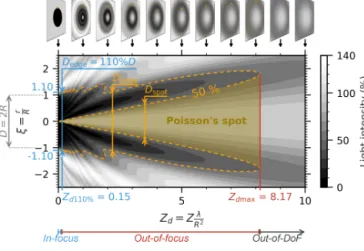
Figure 2, calculated in analogy to Fig. 2 of Korolev et al. (1998), shows the light intensity along a radius of the diffrac-tion pattern produced by an opaque disc with a normalized radial coordinate ξ =Rr as a function of Zd.
With increasing distance Zdfrom the object plane (where
Zd=0), the opaque disc is more and more out-of-focus and
the diffraction pattern shows a Poisson spot which contin-uously increases and an external diameter which generally increases with Zd, albeit with small oscillations for Zd<2.
From Zd=0.15 the disc shadow can appear with a
magnifi-cation greater than 110 %. This arbitrary limit (Knollenberg, 1970) defines the separation of in-focus from out-of-focus images. As Zdcontinues to increase, the diffraction pattern
Figure 2. Intensity level of the diffraction pattern of an opaque disc in Zd–ξ coordinates: the intensity profile along the ξ axis at a
spe-cific Zdrepresents the intensity profile along a section of the
diffrac-tion pattern of an opaque disc at a distance Zd(see the diffraction
pattern for Zd=1.0 in Fig. 1). As Zd increases, the image be-comes less focused and the diameter of the Poisson spot increases. At the 50 % intensity triggering level, the external diameter of the diffraction pattern of the disc shadow can appear with magnifica-tion greater than 110 % from Zd=0.15, which we define as the
arbitrary limit of an in-focus image, and the disc shadow totally dis-appears beyond Zd=8.17.
becomes more and more blurry, and at some point the light intensity no longer falls below a specific triggering level at any point of the pattern. This means for a 50 % intensity trig-gering level of a binary OAP probe that the disc shadow to-tally disappears beyond Zd max=8.17 (Korolev et al., 1998).
This distance delimits the region of the depth of field (DoF) of the particle (Korolev et al., 1991). Beyond this limit, a par-ticle is out-of-DoF and is no longer recorded on a 50 % in-tensity triggering level instrument. As Zmax=R2Zd max/λ,
the DoF increases with the square of the particle size and the inverse of the wavelength.
2.2 Experimental device
The two-dimensional stereo (2D-S) probe (Lawson et al., 2006) is an OAP that records the diffraction pattern of par-ticles illuminated by a laser beam with wavelength λ = 783 nm on a 128-photodiode array. As a particle crosses the laser beam of the instrument, slices of 128 pixels are recorded one after another at a specific frequency which is chosen such that the pixel size in the direction of the moving parti-cle is 10 µm. The size of the pixels in the array direction can slightly vary from one instrument to another. Based on our own calibration using a spinning glass disc with imprinted opaque disc shapes (described further below), we found a mean value of 11.4 µm for the pixel size parallel to the array for the 2D-S used in this study. Note that the 2D-S has been sent to the SPEC Inc. company for a complete check prior to
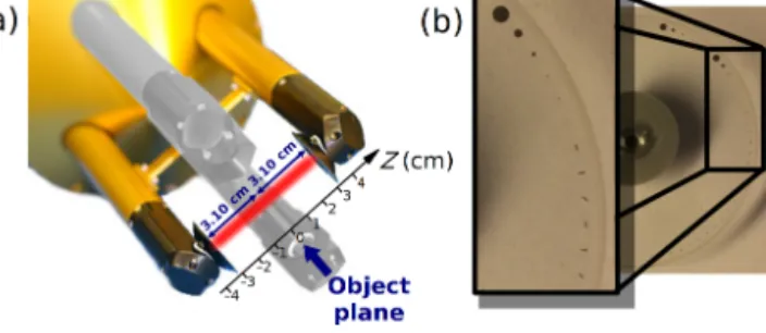
Figure 3. (a) 2D-S probe with a schematic of the laser beam. The probe consists of two pairs of arms allowing measurements in two orthogonal directions. We only consider one couple of arms here. The object plane is located in the middle of the laser beam be-tween the two arms. (b) Spinning disc with imprinted opaque parti-cle shapes.
the tests for this study. Images recorded are monochromatic images based on a 50 % intensity triggering level. The trans-mitting optics consist of a single-mode fiber-coupled diode laser and beam shaping optics (Lawson et al., 2006). Thus, we can assume that a particle is illuminated by a monochro-matic plane wave. The receiving system consists of imaging optics and a linear photodiode array. The imaging optical sys-tem is based on a Keplerian telescope design. The photodiode array is positioned in the focal plane of the back lens (the eye-piece) in the image space. The object plane is the conjugate plane, that is, the focal plane of the front lens (the objective) in the object space. Based on the instrument optics, the ob-ject plane is located in the middle of the laser beam between the two arms of the probe (Fig. 3a).
Therefore, distance Z discussed in the previous section corresponds to the distance of the particle to the object plane (located at Z = 0). The diffraction image of a particle cross-ing the laser beam at Z = x is identical to the diffraction image produced by a particle crossing the laser beam at Z = −x.
Considering opaque discs crossing the 2D-S laser beam, Fig. 4 shows the evolution of the DoF limit Zmaxand the
in-focus limit Z110 % as a function of the variable opaque disc
diameter D.
A particle with D = 500 µm is seen in-focus, i.e., Dedge<
110 %D, as long as the distance of the particle to the ob-ject plane is Z < 1.2 cm. From Z = 1.2 to Z = 3.1 cm (arm limit), the particle is out-of-focus; i.e., the particle is still detected (at least one photodiode triggered), but its image is progressively deformed due to diffraction. For a particle with D = 50 µm, the in-focus zone is very small (Z110%=
0.01 cm) and the particle is no longer detected beyond Zmax=0.65 cm. Particles larger than 109 µm should be
al-ways seen by the 2D-S since the DoF is starting to exceed the distance between the probe arms (6.2 cm). However, particles of that size are potentially observed with more or less im-portant distortion in the out-of-focus domain. Particles larger than 806 µm should be imaged by the 2D-S without
impor-Figure 4. Depth of field (DoF) limit (distance Zmaxfrom the object
plane) separating out-of-DoF and out-of-focus regions, and in-focus limit (distance Z110%from the object plane where the external
di-ameter of the diffraction pattern appears with 110 % magnification) separating out-of-focus and in-focus regions, for an opaque disc with diameter D measured with the two-dimensional stereo (2D-S) probe. The hatched area illustrates the arm limit and the 128-photodiode array size.
tant distortion, since Z110 %>3.1 cm for sizes larger than
806 µm.
In the following third section, we compare theoretical diffraction patterns of different opaque shapes with exper-imental measurements of the 2D-S probe. Therefore, sev-eral spinning glass discs with various chrome opaque par-ticle shapes imprinted on the glass disc surfaces were used (Fig. 3b). This has been performed for opaque disc shapes in the past (e.g., Hovenac and Hirleman, 1991; Reuter and Bakan, 1998) and most recently also for plate and rosette-type particles (Gurganus and Lawson, 2018). Here we present results for two opaque planar particle shapes: rectangle-type shapes which represent the cross section of a columnar particle and “H ”-type shapes which represent the cross section of a capped columnar particle. Particle shapes were imprinted with three different orientations: 0, 45, and 90◦. Note that the chosen shapes represent only one particu-lar projection of a 3-D particle (columnar or capped colum-nar particles) on a 2-D plane.
3 Results
3.1 Comparison of theoretical images with measurements
Figure 5 shows results for a 1 : 2 (width : height) short colum-nar particle with four different sizes (the well-known results for opaque discs are reported in Appendix B).
In each column, on the left-hand side are shown the theoretical 2D-S records and on the right-hand side are shown the images recorded by the 2D-S experimentally. The theoretical 2D-S records are obtained by AST-FFT simulations (Sect. 2.1) with a modeling resolution of 1 µm, 50 % intensity threshold, and subsequently 10 × 11.4 µm
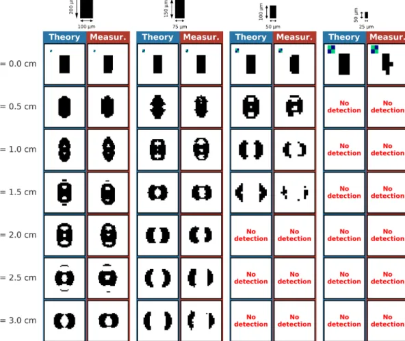
Figure 5. Theoretical and measured 2D-S diffracting patterns of 1 : 2 (width : height) opaque rectangular planar shape particles (short columns) at several distances Z from the object plane. Images are framed according to the particle size; the blue and green target in the first line shows the 2 × 2-pixel scale for the images in the entire column below.
pixelization. Note that images are framed according to the particle size; i.e., smaller particle images are up-scaled with respect to larger ones. Each line shows results for particles at a specific distance Z from the object plane (Z = 0 cm) to a distance very close to the arm of the probe (Z = 3 cm). Results obtained for negative values of Z look very similar (not shown). Note that different particle orientations (0, 90◦; see Sect. 2.2) were chosen for the measurements in order to avoid splitting of a particle into two or more images by the probe’s image separator, at least in one orientation. A strik-ing result is that measurements obtained with the 2D-S probe are in really good agreement with the theoretical diffraction simulation results, not only in terms of diffraction pattern, but also with respect to the DoF limit which is illustrated by the disappearing image at approximately the same Z value in theory and the corresponding measurement. We notice that several Poisson spots can appear in the same particle shadow, as observed for example for the 100 × 200 µm particle passing at Z = 2 cm in both the simulation and the measurement. In contrast to opaque disc particles which preserve their contour shape, columns recorded by the 2D-S
can end up in 2-D images that are very different from a column, as seen for the 75 × 150 µm particle at Z =1.5 cm. The image resembles more a disc with Poisson’s spot than a column. Also, particle images can present small patterns detached from the main particle, as seen at Z = 1.5 and Z =2.5 cm for the 100 × 200 µm particle. Approaching the DoF limit, the columnar particle is split into two symmetrical particles with the shape of a “crescent moon”. The evolution of the particle shape with Z with a 0.01 µm step is shown in the Supplement videos (available here: columnar particle with sizes of 25 × 50 µm (https://doi.org/10.5446/40656), 50 × 100 µm (https://doi.org/10.5446/40658), 75 × 150 µm (https://doi.org/10.5446/40660), and 100 × 200 µm (https://doi.org/10.5446/40662)).
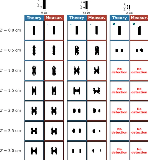
Figure 6 then shows results for a 1 : 4 (width : height) elon-gated column with three different sizes.
Comparison between theory and measurements again shows very good agreement. Also for this crystal geom-etry, diffraction can produce patterns that are very differ-ent compared to the initial shape. In addition, we notice that these patterns look very different than those found
Figure 6. As Fig. 5 for 1 : 4 (width : height) opaque rectangular planar shape particles (elongated columns).
in Fig. 5 for the shorter columns. Here, the diffraction pattern turns into a capped columnar shape as Z in-creases (see, e.g., 75 × 300 µm particle at Z = 3 cm) and ends by splitting into two symmetrical particles when Z approaches the DoF limit (see, e.g., 50 × 200 µm parti-cle with Z > 2 cm). This is also illustrated in the Sup-plement videos (available here: columnar particle with sizes of 25 × 100 µm (https://doi.org/10.5446/40657), 50 × 200 µm (https://doi.org/10.5446/40659), and 75 × 300 µm (https://doi.org/10.5446/40661)).
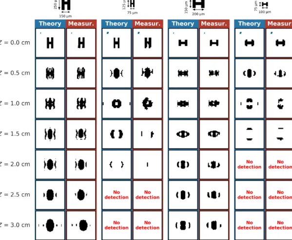
Figure 7 shows results for four capped columnar particles with different ratios and sizes.
Once again, the very good agreement between simu-lated and recorded images is striking. The diffraction pat-tern for one individual capped columnar particle can adopt many different image shapes, as can be seen for example for the 150 × 250 µm capped column. We notice that sev-eral small patterns may be detached from the main parti-cle as a function of distance Z from the object plane. We also notice that capped columnar particles can fall apart into
three distinct “large” parts in the produced binary diffrac-tion image as seen for the 200 × 150 µm particle at Z = 2 cm. The Supplement videos (available here: capped colum-nar particle with sizes of 75 × 125 µm with 25 × 25 µm bar (https://doi.org/10.5446/40652), 100×75 µm with 50×25 µm bar (https://doi.org/10.5446/40653), 150 × 250 µm with 50 × 50 µm bar (https://doi.org/10.5446/40654), and 200×150 µm with 100 × 50 µm bar (https://doi.org/10.5446/40655)) are very helpful for visualizing the evolution of the diffraction pattern.
As a particle moves away from the object plane, we no-tice that its image becomes more and more roundish regard-less of its initial shape. The information of the real shape of the particle ends up being lost as the diffraction patterns progressively adopt a more circular form. This is particu-larly striking on videos. This means that any particle shape far from the object plane produces a more and more circular diffraction pattern which no longer allows us to identify the original shape of the respective particle. See for example the theoretical 75 × 125 µm capped columnar particle diffraction
Figure 7. As Fig. 5 for opaque capped columnar planar shape particles: 250 × 150 µm (external edges) with 50 × 50 µm mid-column, 125 × 75 µm with 25 × 25 µm mid-column, 150 × 200 µm with 50 × 100 µm mid-column, and 75 × 100 µm with 25 × 50 µm mid-column.
pattern at Z = 1 cm (Fig. 7) or the theoretical and measured 75 × 150 µm short column diffraction pattern at Z = 1.5 cm (Fig. 5). Depending on the initial shape, the binary diffrac-tion pattern is generally broken into two, sometimes three image parts of similar sizes when approaching the DoF limit. Depending on the orientation of the particle, these two or three particles can be interpreted as different particles by the 2D-S probe. Indeed, the 2D-S probe stores a new particle as soon as a slice with 128 white pixels (image separator set by probe) is found. Because these two or three “particles” are registered as very close particles in time, algorithms will gen-erally remove these particles from the data set, thereby con-sidering them to be particles generated from shattering (Field et al., 2006). This can create significant differences when par-ticles are not properly recorded or deleted by the shattering algorithm before reaching the theoretical DoF limit. For ex-ample, the 75 × 150 µm short columnar particle (Fig. 5; sec-ond column) might be removed by the shattering algorithm beyond Z = 1.59 cm (see video in the Supplement available here: https://doi.org/10.5446/40660), whereas its theoretical DoF exceeds the distance between the arms. Therefore, it se-riously affects the sample volume which is based on the DoF
limit (Korolev et al., 1991) and consequently affects the re-trieved concentrations.
Another interesting remark based on these results is that an out-of-focus image of a distinct particle shape can closely resemble another particle of a very different shape. As an example, note that the diffraction pattern of a 75 × 300 µm columnar particle at Z = 2.5 cm (Fig. 6) looks a lot like an in-focus capped columnar particle in the object plane. Also, the diffraction pattern of a 75×125 µm capped columnar particle at Z = 1 cm (Fig. 7) looks like a disc with Poisson’s spot, meaning that an out-of-focus capped columnar ice particle can be interpreted as a droplet faintly out-of-focus.
3.2 Theoretical evolution of the equivalent and maximum particle diameters
In this section, we present some diffraction simulation results for four chosen particle shapes to illustrate the evolution of the particle diameter, including uncertainty evaluation. Our purpose here is neither to present an exhaustive list of results related to each shape nor to quantify the uncertainty of the probe in an absolute manner.
The size of the particle from a 2-D image has no abso-lute definition. Several definitions are used in the literature with different pros and cons depending on the objective of the study. In the study presented here, we illustrate results with two commonly used particle size definitions: the surface-equivalent diameter Deq and the maximum diameter Dmax.
Deqis defined as the diameter of a disc with the same surface
as the analyzed particle image. Dmaxis defined as the
diam-eter of the smallest circle encompassing the particle image (e.g., Chrystal, 1885; Welzl, 1991; Heymsfield et al., 2013; Wu and McFarquhar, 2016). Note that all triggered pixels of the image are considered here for the computation of Deqand
Dmax, even when the pattern is split into several fragments
(see Sect. 3.1).
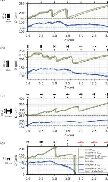
Figure 8 shows the theoretical evolution of Deq(solid blue
line) and Dmax(solid green line), applying the 50 % threshold
to a simulated 1×1 µm pixel image pattern, as a function of Z for four different particles: two rectangles with very similar true Deq(119.7 and 112.8 µm) but different aspect ratios (1 :
2 and 1 : 4, or short and elongate columns, respectively) and two capped column-type particles with the same shape but different sizes.
Dashed lines show the true Deq and Dmaxparticle
diam-eters. The produced binary images from diffraction simu-lations are presented on top of each sub-figure of Fig. 8 for a few distinct distances of Z (Z = 0, 0.5, 1.0, . . . , and 3.0 cm). Blue and green shadow areas in this figure show Deqand Dmaxfor the theoretical records by the 2D-S (pixel
of 10 × 11.4 µm). Indeed, a spread for each size would ap-pear due to the discrete pixel effect. As a photodiode needs to be shadowed from at least 50 % light intensity to be trig-gered, the number of triggered pixels will depend on the po-sition of the particle shadow on the photodiode array of the probe. To account for this discrete pixel effect, particles are systematically shifted over one 10 × 11.4 µm 2D-S pixel by increments of 1 µm in both directions. This discrete pixel ef-fect is illustrated in the Supplement video (available here: https://doi.org/10.5446/40663), showing the 150 × 250 µm capped columnar particle at Z = 0.5 cm. We note that the pixels at the edge can be triggered or not as the particle is shifted, which then affects the particle size.
At first, we discuss diffraction simulation results of short and elongated columns presented in Figs. 8a and 8b. Both figures illustrate the evolution of Deqand Dmaxas both
parti-cles pass the laser beam between Z = 0 and Z = 3.1 cm. The evolution of Deqis rather smooth with varying Z, compared
to Dmaxevolution, which is much more oscillating. Still, both
columnar particles have a comparable true Deq (119.7 µm
versus 112.8 µm), and both Dmax and Deq evolution show
some nice similarities. Nevertheless, between Z = 0 and Z = 3.1 cm, for the short column (Fig. 8a) Deqand Dmax from
theoretical binary images are always greater than the corre-sponding true Deq (119.7 µm) and Dmax(168.6 µm) values,
whereas the Deq and Dmax retrieved from binary
diffrac-tion images of the elongated column (Fig. 8b) are lying on
Figure 8. Evolution of the theoretical Deq (solid blue line) and
Dmax(solid green line) of the diffracting image of a particle as a
function of Z (with a 50 % intensity threshold), compared to the true Deq(dashed blue line) and the true Dmax(dashed green line)
of the particle. Binary images from diffraction patterns added on top of four figures for several Z distances. Blue and green shadow areas are the theoretical records by the 2D-S with the uncertainty due to the position of the particle in front of the photodiode array. Only 0◦ particle orientation is considered here.
either side of the theoretical value lines, Deq=112.8 and
Dmax=207.4 µm. Repeated abrupt decreases in measured
Dmax are related to changes in the outer binary pixel
en-sembles of the diffraction pattern which are drifting away from the particle center as Z increases. This then leads to sudden loss of outer pixel and related decrease in Dmax.
De-taching pixel ensembles are frequently observed, with two to three produced sub-images stemming from the diffraction pattern of one particle. This can lead to virtually large Dmax
(e.g., Dmax=240 µm for the short column at Z = 3.0 cm
corresponding to the true Dmaxof 168.6 µm).
Secondly, the two capped column-type particles are dis-cussed. With increasing Z, the size of the larger capped col-umn (Fig. 8c) increases for both diameter definitions Deqand
Dmax. Deq of this particle when observed at a distance of
3 cm is about 210 µm, which exceeds by 50 µm the true Deq
of 159.6 µm of the particle. Also, Dmax generally increases
with increasing Z, however with few transient smaller diam-eter decreases at some distances depending on the evolution of the diffraction pattern details at the edges of the binary par-ticle image. The smaller capped columnar parpar-ticle (Fig. 8d) disappears before reaching Z = 3.1 cm (arm limit). The ap-parent particle size first grows with Z, then shrinks contin-uously in terms of Deq (more abruptly in terms of Dmax),
followed by another phase of slight increase in Dmax, before
the particle then completely disappears in both diameter def-initions at a distance Z of roughly 1.8 cm. Again, it can be noticed that in general Deqchanges more gently with Z, as
compared to Dmax. Close to the DoF limit, which is estimated
from diffraction simulations for the particle in Fig. 8d as the position Z where the binary image disappears (roughly at Z =1.8 cm), Deqis underestimated, whereas Dmax
contin-ues to be overestimated as the particle image is formed by a few distant pixels. We note also that DoF limits from cal-culations of Zmax=D2Zd max/(4λ) produces different DoF
limit values for Deq and Dmaxsize definitions for the same
particle (DMT, 2009; SPEC, 2011). The DoF limit values are Zmax=1.66 (using Deq) and Zmax=4.13 cm (using Dmax).
These different DoF limit estimations (factor of 2.5 between both calculations) using the above equation for this particle means different sample volumes, and finally different con-centrations. For this particle, using the DoF limit estima-tions with Deqwould be closer to the DoF limit (Z = 1.8 cm)
found from diffraction simulation. Moreover, as the uncer-tainty in Deq for out-of-focus particles is relatively small
(Table 2) compared to Dmax (Fig. 8), it should be a
rela-tively good option to estimate the DoF limit. However, our arbitrary diameter definition used in the classical DoF limit calculation remains questionable, since ice particles are pri-marily non-spherical.
Furthermore, for both columnar and capped columnar pticles, it is evident that the discrete pixel effect (shadow ar-eas) is almost negligible with respect to the diameter vari-ability along the Z distance according to the diffraction sim-ulations.
Finally, Table 1 summarizes Fig. 8 in terms of maximum, minimum, and average Deq and Dmax diameters over the
whole distance between the two arms of the 2D-S probe com-pared to the true Deqand Dmax. For these four particles, we
note that uncertainty for particles with a DoF limit beyond the arm limit spans from −23 % to +35 % in Deqand from
−15 % to +48 % in Dmax. For the smallest particle,
uncer-tainty spans from −85 % to +39 % in Deqand from −88 %
to +69 % in Dmax. For this small particle, with a DoF limit
smaller than the arm limit, the lower bound of the uncertainty has been calculated for a 1-pixel particle.
3.3 Comparison of theoretical statistics with measurements
In this section, we compare particle size distributions re-trieved theoretically from diffraction pattern simulations and experimentally measured by the 2D-S probe. For the mea-surements, a spinning disc (Fig. 3b) has been utilized with imprinted short columnar particles shown in Fig. 5. The spin-ning disc contains four different particle sizes, all of them imprinted in three different orientations (0, 45, and 90◦) and repeated six times. Therefore, each particle size should be seen 18 times at each revolution of the spinning disc. We simulate and measure 10 s of disc spinning at 108.6 ± 0.2 rps (≈ 9.5 m s−1in equivalent particle speed), which should re-sult for each of the four short columns in about 19 500 im-ages; 9.5 m s−1 already represents the maximum equivalent speed of particles on the rotating disc, which is small com-pared to aircraft speeds and therefore does not allow us to study possible effects of electronic response time related to disc speed.
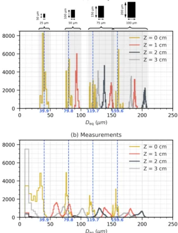
Figure 9a shows theoretical results obtained from diffrac-tion patterns by simulating each of the four particles 19 500 times.
Each of the three orientations (0, 45, and 90◦) accounts for one-third of the contribution of each of the four particles to the particle size distribution. The true equivalent diameter Deqof a 100 × 200 µm particle is 159.6 µm. At Z = 0 cm, the
particle image projected onto the photodiode array is undis-torted. However, we see in Fig. 9a that the diameter is not re-trieved perfectly and is also slightly varying. Depending on the position of the shadow particle projected onto the pho-todiode array, Deq can vary from 152 to 169 µm, which is
due to taking into account the discrete pixel effect. There-fore, even in the best case when particles cross the laser beam of the 2D-S in the object plane and without any noise, this particle can be recorded with an uncertainty in Deq of
up to 6 %, only due to the discrete pixel effect. By mov-ing the 100 × 200 µm particle away from the object plane to Z =1 cm, then 2 cm, and finally 3 cm, we notice that Deq
first starts to increase, and then decreases. The described be-havior depends on particle size and shape, but has a common feature: particle Deqgenerally starts to increase and then
de-creases until it disappears when reaching the DoF limit, as shown for the small capped column in Fig. 8d.
Figure 9b shows the size distribution of the four short columnar particles measured by the 2D-S. At Z = 0 cm, the number of counted particles (yellow curve with four dis-tinct modes attributed to four particle sizes) for the four par-ticle sizes (from larger to smaller ones) is 19 488, 19 484, 19 464, and 29 490. Note that most of the very small parti-cles (< 4 pixels at Z = 0 cm) are due to dust on the spinning disc (the first four bars of the orange histogram). The
num-Table 1. True Deqand Dmaxof particles shown in Fig. 8 compared with the minimum, maximum, and average theoretical Deqand Dmax
over the whole distance between the two arms of the 2D-S probe. The minimum and maximum relative errors with respect to true Deqand
Dmaxare shown in brackets behind minimum and maximum diameter values.
Column 75 × 150 µm Column 50 × 200 µm Capped column 200 × 150 µm Capped column 100 × 75 µm True Deq 119.7 µm 112.8 µm 159.6 µm 79.8 µm Mean Deq 139.4 µm 124.2 µm 194.8 µm 48.3 µm Min Deq 114.9 µm (−4 %) 86.9 µm (−23 %) 157.1 µm (−2 %) 12.0 µm (= 1 pixel) (−85 %) Max Deq 158.5 µm (+32 %) 148.5 µm (+32 %) 214.8 µm (+35 %) 111.1 µm (+39 %) True Dmax 168.6 µm 207.4 µm 251.4 µm 125.8 µm Mean Dmax 200.8 µm 205.8 µm 301.9 µm 91.8 µm
Min Dmax 163.9 µm (−3 %) 175.6 µm (−15 %) 248.9 µm (−1 %) 15.2 µm (= 1 pixel) (−88 %)
Max Dmax 244.6 µm (+45 %) 241.5 µm (+16 %) 373.0 µm (+48 %) 213.1 µm (+69 %)
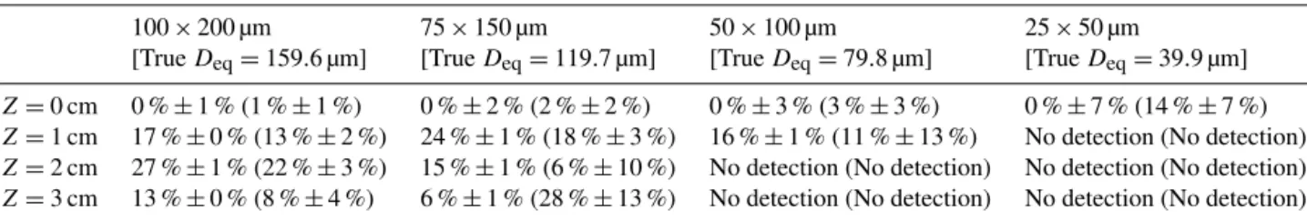
Table 2. Theoretical (measured) relative uncertainty 1Deq=ε ± σfor the four opaque short columnar shape particles shown in Fig. 9 with
three orientations (0, 45, and 90◦) of equal probability. ε represents the relative mean error and σ its relative standard deviation (due to the pixel effect) from the true Deq. For the 25 × 50 µm short columnar particle at Z = 0, only images with more than 4 pixels are considered.
100 × 200 µm 75 × 150 µm 50 × 100 µm 25 × 50 µm
[True Deq=159.6 µm] [True Deq=119.7 µm] [True Deq=79.8 µm] [True Deq=39.9 µm]
Z =0 cm 0 % ± 1 % (1 % ± 1 %) 0 % ± 2 % (2 % ± 2 %) 0 % ± 3 % (3 % ± 3 %) 0 % ± 7 % (14 % ± 7 %) Z =1 cm 17 % ± 0 % (13 % ± 2 %) 24 % ± 1 % (18 % ± 3 %) 16 % ± 1 % (11 % ± 13 %) No detection (No detection) Z =2 cm 27 % ± 1 % (22 % ± 3 %) 15 % ± 1 % (6 % ± 10 %) No detection (No detection) No detection (No detection) Z =3 cm 13 % ± 0 % (8 % ± 4 %) 6 % ± 1 % (28 % ± 13 %) No detection (No detection) No detection (No detection)
ber of counted particles smaller than 4 pixels at Z = 0 cm is 12 029. At Z = 0 cm, the four observed particle modes can be clearly attributed to the four different short columnar par-ticle sizes. Distributions show reasonably narrow peaks. The position of the individual peaks is on average 5 µm below the expected respective true Deq, which is half of the pixel
size. Experimentally, the discrete photodiodes in the array and the 50 % occultation criterion introduce a digitization un-certainty of roughly 1 size resolution (= 10 µm for the 2D-S) depending upon where the particle passes across the array (Baumgardner et al., 2017). We recall also that we found a mean value of 11.4 µm for the pixel size along the photo-diode array based on our own calibration using a spinning glass disc with a printed opaque disc shape of 800 µm in di-ameter. Smaller size effects could be that different particles cross different photodiodes at different positions of the lin-ear photodiode array, which is due to the fact that the ro-tation axis and the spinning glass disc center are not per-fectly coaxial. Indeed, all photodiodes may not have an iden-tical response. With increasing values of Z > 0 cm, distri-butions of individual modes are getting broader. Whereas at Z =1 cm the three larger particles are observed, at Z = 2 and Z = 3 cm solely the two larger particles have their DoF beyond these distances. For the larger short columnar par-ticle (100 × 200 µm), the four peaks corresponding to the four distances Z are well located compared to theoretical re-sults, and each peak contains 19 500 ± 20 records. The sec-ond larger short columnar particle (75×150 µm) shows quite
good agreement with simulations for peak position at Z = 1 and Z = 2 cm, and contains 19 514 and 18 548 records, re-spectively. The missing particles at Z = 2 cm appear in the very small mode centered around 90 µm. In this small mode, we found 1924 particles which correspond to 962 particles split into two parts (Fig. 5). Results at Z = 3 cm show two distinct modes centered on 72 and 102 µm, well below the theoretical peak at 128 µm. The 102 µm mode is due to split particles with 45 and 90◦orientations which were not sep-arated by the probe into two images. This mode is not cen-tered as the theoretical mode (128 µm) because the split parti-cles show fewer triggered pixels in measurements compared to theoretical simulations (see Fig. 5). This finding may be due to the fact that the probe’s 50 % threshold does not per-fectly coincide with the theoretical 50 % threshold. This ef-fect may particularly impact the resulting probe images when approaching the DoF limit. The 72 µm mode is due to split particles with 0◦ orientation such that a separator can be set by the probe which generates two smaller particles. The sum of the record number in the larger mode corresponding to 45 and 90◦ orientations (13 090) and half of the smaller mode corresponding to 0◦orientation (6403) yields in total 19 483. The 50×100 µm short column also shows two modes at Z =1 cm for the same reason. Particles smaller than 40 µm in Deqat Z ≥ 1 cm are not dust particles on the spinning disc
since their DoF limit is smaller than Z = 1 cm. Actually, it can be seen from visual inspection of consecutive images that these small particles result from the separation of very small
Figure 9. (a) Theoretical 2D-S Deqsize distribution for opaque
short columnar particles shown in Fig. 5. Each particle at each Z is simulated 19 500 times with three orientations (0, 45, and 90◦) and with different positions over the photodiode array. Uncertainty is then due to diffraction and to the discrete pixel effect. (b) 2D-S size distribution for the same four short columnar particles imprinted with three orientations (0, 45, and 90◦) on the spinning disc.
patterns from the main particles at the edge of the diffraction image. This effect is particularly striking at Z = 3 cm and is consistent with findings published in the literature. For ex-ample, fragmented diffraction patterns of spherical droplets traversing the sample area near the edges of the DoF were shown in the work by Korolev (2007); diffraction fringes around out-of-focus images measured by CIP were under-scored by Korolev and Field (2015). “Reacceptance” algo-rithms (e.g., Korolev and Field, 2015; McFarquhar et al., 2017a) should address rigorously the problem of intact, i.e., not shattered, but fragmented particles.
We stated in Sect. 3.2 that the uncertainty in Deq due to
diffraction in the out-of-focus region is far more important than the discrete pixel effect uncertainty. Table 2 shows the theoretical and measured uncertainty 1Deq=ε ± σ for the
four opaque short columnar particles shown in Fig. 9, where ε represents the relative mean error and σ its relative stan-dard deviation, both with respect to the true Deq. We notice
that standard deviation σ , both in theory and measurements,
is generally small compared to the mean error ε for out-of-focus particles, except when measurements present a two-modal distribution as seen for the 75 × 150 µm short colum-nar particle at Z = 2 and Z = 3 cm, and for the 50×100 µm short columnar particle at Z = 1 cm. For these specific cases, we notice that particles with true Deq larger than 100 µm
can have uncertainties up to 27 % ± 1 % theoretically and up to 28 % ± 13 % in measurements when split particles ap-pear. Particles with true Deq smaller than 100 µm (the two
smaller short columns of Fig. 5) do not show uncertainties larger than derived for the two larger particles in this table because uncertainties are solely quantified for a few discrete Zdistances. Uncertainties for particles smaller than 100 µm would dramatically increase as Z approaches the DoF limit as shown in Fig. 8d.
4 Conclusions
We presented in this study a first comparison of theoretical diffraction simulations of non-spherical cloud particles and respective image responses of OAP probes. First, the angular spectrum method has been applied to obtain diffraction pat-terns of spherical and non-spherical particles when viewed at specific distances from the object plane. For exemplary cloud particle shapes, diffraction simulations help in studying how the diameter retrieved from 2-D binary images is impacted by the distance from the object plane where the particle crosses the laser beam. Furthermore, we compared theoretical results with experimental measurements made with a 2D-S probe. The main results are the following.
1. The diffraction image formed by an opaque planar par-ticle, illuminated perpendicularly by a monochromatic coherent homogeneous plane wave, at a distance Z be-yond the object plane can be computed using angular spectrum theory.
2. Circular particles with diameters larger than 806 µm are theoretically always recorded by the 2D-S probe with-out noteworthy size deformation (< 10 %).
3. Circular particles with diameters larger than 109 µm are theoretically always recorded by the 2D-S (potentially with huge deformation), whereas particles smaller than 109 µm theoretically are no longer detectable once out-of-DoF.
4. Theoretical diffraction simulations allow us to estimate DoF limits (as from Figs. 5–7 and 9d) which are consis-tent with the measurements.
5. Diffraction images of out-of-focus particles are some-times very similar to other in-focus particle shapes. As an example, we observe that an out-of-focus elongated columnar ice particle can be interpreted as an in-focus capped columnar ice particle. An out-of-focus capped
column can also be viewed as a droplet faintly out-of-focus.
6. In general, diffraction images of all kinds of particle shapes consecutively lose their real shape information with increasing distance Z. Diffraction images show cir-cular fringes, which is the reason why particle image edges tend to arch when Z increases.
7. Due to the finite pixel size of the probe and the 50 % oc-cultation threshold, there is an uncertainty in the particle size measurements, even when Z = 0 cm. For the four short columnar particles presented in this study, this digitization uncertainty is less than 7 % in Deq.
How-ever, uncertainty for an out-of-focus particle is far more important and easily reaches several tens of percent of its diameter. These uncertainties are well retrieved ex-perimentally. Also, experimental size distributions are broader than theoretical distributions due to optical and electronic noises. According to the Baumgardner et al. (2017) overview paper, OAP probes are considered to size correctly particles smaller than 100 µm and larger than 100–200 µm to ±50 % and ±20 %, respectively. For the three largest short columnar particles with true Deqand true Dmaxof 112.8–159.6 and 168.6–251.4 µm,
respectively, we found for the 2D-S simulations an un-certainty that spans from −23 % to +35 % in Deqand
from −15 % to +48 % in Dmax. For the smallest
parti-cle, with a DoF limit smaller than the arm limit, with true Deq of 79.8 µm and true Dmax of 125.8 µm, we
found an uncertainty that spans from −85 % to +39 % in Deqand from −88 % to +69 % in Dmax.
8. The intercomparison of theoretical and experimental Deqresults for the four short columnar particles at
dis-tinct distances Z shows a rather good agreement in re-trieved uncertainties with respect to true Deq, which is
primarily driven by the diffraction effect and to a minor extent by the discrete pixel effect. This agreement dete-riorates when particle patterns are separated into two or more images by the probe.
The good agreement between the simulated and measured diffraction patterns (see Figs. 5, 6, 7, and B1) suggests that the laser beam of the used 2D-S probe is well collimated and the use of the plane-wave approximation is well founded. Fu-ture investigations, especially concerning grayscale thresh-olds, could take into account properties of the laser beam and the optical system. For example, angular spectrum theory was used in the work by Hayman et al. (2016) to simulate the diffraction pattern of an opaque disc illuminated by an ellip-tical Gaussian beam, where an opellip-tical receiver point spread function was considered.
This study suggests that the incorrect particle sizing of cloud particles by OAPs is predominantly due to the diffrac-tion effect in the out-of-focus region. Reducing the distance
between the probe arms allows one to reduce diffraction ef-fects, but simultaneously reduces the sampling volume. In order to reduce the sizing uncertainty, it would be extremely useful to get a direct and independent measure of the dis-tance Z at which a cloud particle crosses the laser beam of the probe. The knowledge of Z would allow one to re-move an unknown in inversion techniques to better estimate the true particle size of non-spherical particles in analogy to what has been suggested by Korolev (2007) for spheri-cal particles. At the moment, we think that the simulation of diffraction images of various cloud particle shapes will help us to better characterize OAP uncertainties in terms of small particle concentrations. This topic has not been in the scope of this study. Small particle concentrations can be extremely wrong, which has its origins in artificial small particles from diffraction, shattering, photodiode malfunctioning, and other noise. Each artifact’s small particle is assigned a very small DoF and thus sample volume (Bansemer and Heymsfield, 2018), leading to extremely overestimated small particle con-centrations. Finally, assuming that real 3-D opaque parti-cles produce diffraction images analogous to those obtained with their plane cross-section shape, the diffraction simula-tion method presented in this study will allow us to conceive an OAP simulator using numerical 3-D particles which can be randomly oriented. However, it should be noted that this method does not take into account reflection and refraction effects of the light which can be non-negligible for ice cloud particles.
Data availability. The data from this study can be obtained by con-tacting the corresponding author of this article.
Appendix A: Angular spectrum theory
In this Appendix, we use the same terminology as has been used in Sect. 3.10 of the classic textbook by Goodman (1996). Suppose that a monochromatic plane wave is propa-gating in the positive Z direction and the complex field across the Z = 0 plane is represented by Ui(x, y,0). A diffracting
structure is introduced in the plane Z = 0. The amplitude transmittance function tA(x, y) is the ratio of the
transmit-ted field amplitude Ut(x, y,0) to the incident field amplitude
Ui(x, y,0) at each position (x, y) in the Z = 0 plane; that is,
Ut(x, y,0) = tA(x, y)Ui(x, y,0). (A1)
In this work, the amplitude transmittance function tA(x, y)
is defined as follows: tA(x, y) =
(
1 if outside the opaque shape,
0 if in the opaque shape, (A2) and corresponds to the binary matrix representing the studied opaque shape.
In the Fourier domain, the angular spectrum of Ut(x, y,0)
is
A(fx, fy,0) = +∞
Z Z
−∞
Ut(x, y,0)e−i2π(fxx+fyy)dxdy. (A3)
The angular spectrum of U (x, y, z) at Z = z is given by a solution of the differential equation which represents the Helmholtz equation in the Fourier domain (Ersoy, 2007). This solution can be written as
A(fx, fy, z) = A(fx, fy,0)H (fx, fy), (A4)
where H (fx, fy) = e iz
q
k2−4π2(f2
x+fy2)under the condition of
homogeneous waves (k2>4π2(fx2+fy2)), which is the case in this study. Applying an inverse Fourier transform gives the resulting wave field at the distance Z = z:
U (x, y, z) =
+∞
Z Z
−∞
A(fx, fy, z)e−i2π(fxx+fyy)dfxdfy. (A5)
The diffraction pattern of the particle is then given by the intensity at Z = z: I (x, y, z) = U (x, y, z)2.
Finally, a simple low-pass filter can be used to remove spu-rious noisy high frequencies.
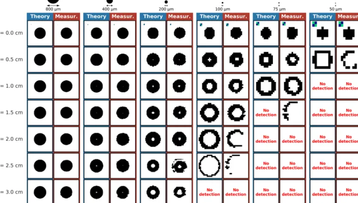
Appendix B: Comparison of theoretical diffraction patterns and measurements of disc shape particles on a spinning disc.
Figure B1. As Fig. 5 for opaque disc shape particles. Videos in the Supplement are available here: circular particle with radii of 25 (https://doi.org/10.5446/40646), 37.5 (https://doi.org/10.5446/ 40647), 50 (https://doi.org/10.5446/40648), 100 (https://doi.org/ 10.5446/40649), 200 (https://doi.org/10.5446/40650), and 400 µm (https://doi.org/10.5446/40651).
Supplement. Image sequences of diffraction patterns for particles at increasing distance from the object plane have been added as a Supplement. All videos are from the series “Simulations of cloud particle diffraction pattern” (Vaillant de Guélis, 2019) available on the TIB AV-Portal at https://av.tib.eu/series/627/simulations+of+ cloud+particle+diffraction+pattern. The supplement related to this article is available online at: https://doi.org/10.5194/amt-12-2513-2019-supplement.
Author contributions. TVdG wrote the manuscript. TVdG and VS performed the theoretical part. CG and BL conceived the test bench. TVdG made the experimental measurements. RD wrote the script to read the 2D-S raw data file. All the authors contributed discussion and feedback essential to the study.
Competing interests. The authors declare that they have no conflict of interest.
Acknowledgements. We would like to thank the FEMTO-ST Insti-tute (UMR 6174) for conceiving the spinning glass discs. This work has been financially supported by the French government space agency CNES.
Review statement. This paper was edited by Wiebke Frey and re-viewed by Darrel Baumgardner and one anonymous referee.
References
Bacon, N. J., Swanson, B. D., Baker, M. B., and Davis, E. J.: Breakup of levitated frost particles, J. Geophys. Res.-Atmos., 103, 13763–13775, https://doi.org/10.1029/98JD01162, 1998. Baker, B., Mo, Q., Lawson, R. P., O’Connor, D., and Korolev,
A.: Drop Size Distributions and the Lack of Small Drops in RICO Rain Shafts, J. Appl. Meteorol. Clim., 48, 616–623, https://doi.org/10.1175/2008JAMC1934.1, 2009.
Bansemer, A. and Heymsfield, A.: A Multi-Instrument Comparison of Small Ice Particle Size Distributions Measured from Aircraft, in: 15th Conference on Cloud Physics/15th Conference on At-mospheric Radiation, Vancouver, BC, Canada, 9–13 July, 2018. Baumgardner, D., Abel, S. J., Axisa, D., Cotton, R., Crosier, J.,
Field, P., Gurganus, C., Heymsfield, A., Korolev, A., Krämer, M., Lawson, P., McFarquhar, G., Ulanowski, Z., and Um, J.: Cloud Ice Properties: In Situ Measurement Challenges, Meteor. Mon., 58, 9.1–9.23, https://doi.org/10.1175/AMSMONOGRAPHS-D-16-0011.1, 2017.
Boucher, O., Randall, D., Artaxo, P., Bretherton, C., Fein-gold, G., Forster, P., Kerminen, V.-M., Kondo, Y., Liao, H., Lohmann, U., Rasch, P., Satheesh, S. K., Sherwood, S., Stevens, B., and Zhang, X. Y.: Clouds and aerosols, in: Climate change 2013: the physical science basis. Contribu-tion of Working Group I to the Fifth Assessment Report of the Intergovernmental Panel on Climate Change,
Cam-bridge University Press, UK and New York, USA, 571–657, https://doi.org/10.1017/CBO9781107415324.016, 2013. Cantrell, W. and Heymsfield, A.: Production of Ice in
Tropo-spheric Clouds: A Review, B. Am. Meteorol. Soc., 86, 795–808, https://doi.org/10.1175/BAMS-86-6-795, 2005.
Cho, H. R., Iribarne, J. V., and Richards, W. G.: On the orientation of ice crystals in a cumulonimbus cloud, J. Atmos. Sci., 38, 1111–1114, https://doi.org/10.1175/1520-0469(1981)038<1111:OTOOIC>2.0.CO;2, 1981.
Chrystal, M.: Sur le problème de la construction du cercle minimum renfermant n points donnés d’un plan, B. Soc. Math. Fr., 13, 198– 200, https://doi.org/10.24033/bsmf.303, 1885.
Connolly, P. J., Flynn, M. J., Ulanowski, Z., Choularton, T. W., Gallagher, M. W., and Bower, K. N.: Calibration of the Cloud Particle Imager Probes Using Calibration Beads and Ice Crystal Analogs: The Depth of Field, J. Atmos. Ocean. Tech., 24, 1860– 1879, https://doi.org/10.1175/JTECH2096.1, 2007.
DeMott, P. J., Hill, T. C. J., McCluskey, C. S., Prather, K. A., Collins, D. B., Sullivan, R. C., Ruppel, M. J., Mason, R. H., Irish, V. E., Lee, T., Hwang, C. Y., Rhee, T. S., Snider, J. R., McMeeking, G. R., Dhaniyala, S., Lewis, E. R., Wentzell, J. J. B., Abbatt, J., Lee, C., Sultana, C. M., Ault, A. P., Ax-son, J. L., Diaz Martinez, M., Venero, I., Santos-Figueroa, G., Stokes, M. D., Deane, G. B., Mayol-Bracero, O. L., Grassian, V. H., Bertram, T. H., Bertram, A. K., Moffett, B. F., and Franc, G. D.: Sea spray aerosol as a unique source of ice nu-cleating particles, P. Natl. Acad. Sci. USA, 113, 5797–5803, https://doi.org/10.1073/pnas.1514034112, 2016.
DMT: Single particle imaging, Data analysis user’s guide, DOC-0223, Rev. A, Tech. Rep., 34 pp., 2009.
Ersoy, O. K.: Diffraction, Fourier optics and imaging, John Wiley & Sons, Hoboken, New Jersey, USA, 2007.
Field, P. R., Heymsfield, A. J., and Bansemer, A.: Shattering and Particle Interarrival Times Measured by Optical Array Probes in Ice Clouds, J. Atmos. Ocean. Tech., 23, 1357–1371, https://doi.org/10.1175/JTECH1922.1, 2006.
Field, P. R., Lawson, R. P., Brown, P. R. A., Lloyd, G., West-brook, C., Moisseev, D., Miltenberger, A., Nenes, A., Blyth, A., Choularton, T., Connolly, P., Buehl, J., Crosier, J., Cui, Z., Dearden, C., DeMott, P., Flossmann, A., Heymsfield, A., Huang, Y., Kalesse, H., Kanji, Z. A., Korolev, A., Kirchgaessner, A., Lasher-Trapp, S., Leisner, T., McFarquhar, G., Phillips, V., Stith, J., and Sullivan, S.: Secondary Ice Production: Current State of the Science and Recommendations for the Future, Meteor. Mon., 58, 7.1–7.20, https://doi.org/10.1175/AMSMONOGRAPHS-D-16-0014.1, 2017.
Gardiner, B. A. and Hallett, J.: Degradation of in-cloud forward scattering spectrometer probe mea-surements in the presence of ice particles, J. Atmos. Ocean. Tech., 2, 171–180, https://doi.org/10.1175/1520-0426(1985)002<0171:DOICFS>2.0.CO;2, 1985.
Gaskill, J. D.: Linear systems, Fourier transforms, and optics, Wi-ley, New York, USA, 1978.
Goodman, J. W.: Introduction to Fourier optics, McGraw-Hill, New York, USA, 2nd Edn., 1996.
Gurganus, C. and Lawson, P.: Laboratory and Flight Tests of 2D Imaging Probes: Toward a Better Understanding of Instru-ment Performance and the Impact on Archived Data, J. Atmos.
Ocean. Tech., 35, 1533–1553, https://doi.org/10.1175/JTECH-D-17-0202.1, 2018.
Hallett, J. and Mossop, S. C.: Production of secondary ice particles during the riming process, Nature, 249, 26–28, https://doi.org/10.1038/249026a0, 1974.
Hayman, M., McMenamin, K. J., and Jensen, J. B.: Response Time Characteristics of the Fast-2D Optical Array Probe Detector Board, J. Atmos. Ocean. Tech., 33, 2569–2583, https://doi.org/10.1175/JTECH-D-16-0062.1, 2016.
Heymsfield, A. J., Schmitt, C., and Bansemer, A.: Ice Cloud Particle Size Distributions and Pressure-Dependent Terminal Velocities from In Situ Observations at Temperatures from 0◦to −86◦C, J. Atmos. Sci., 70, 4123–4154, https://doi.org/10.1175/JAS-D-12-0124.1, 2013.
Hirleman, E. D., Holve, D. J., and Hovenac, E. A.: Calibration of single particle sizing velocimeters using photomask reticles, in: 4th International Symposium on Applications of Laser Anemom-etry to Fluid Mechanics, Lisbon, Portugal, 11–14 July, 6–10, 1988.
Hovenac, E. A.: Use of rotating reticles for calibration of single par-ticle counters, International Congress on Applications of Lasers and Electro-Optics, Arlington, VA, USA, 10–13 November 1986, 58, 129–134, https://doi.org/10.2351/1.5057795, 1986.
Hovenac, E. A. and Hirleman, E. D.: Use of Rotating Pinholes and Reticles for Calibration of Cloud Droplet Instrumentation, J. Atmos. Ocean. Tech., 8, 166–171, https://doi.org/10.1175/1520-0426(1991)008<0166:UORPAR>2.0.CO;2, 1991.
Hovenac, E. A., Hirleman, E. D., and Ide, R. F.: Calibration and sample volume characterization of PMS optical array probes, in: International Conference on Liquid Atomisation and Spray Sys-tems, Imperial College, London, 8–10 July, 1985.
Joe, P. and List, R.: Testing and performance of two-dimensional optical array spectrometers with greyscale, J. At-mos. Ocean. Tech., 4, 139–150, https://doi.org/10.1175/1520-0426(1987)004<0139:TAPOTD>2.0.CO;2, 1987.
King, W. D.: Air flow and particle trajectories around air-craft fuselages, IV: Orientation of ice crystals, J. At-mos. Ocean. Tech., 3, 433–439, https://doi.org/10.1175/1520-0426(1986)003<0433:AFAPTA>2.0.CO;2, 1986.
Knollenberg, R. G.: The Optical Array: An Alternative to Scat-tering or Extinction for Airborne Particle Size Determination, J. Appl. Meteorol., 9, 86–103, https://doi.org/10.1175/1520-0450(1970)009<0086:TOAAAT>2.0.CO;2, 1970.
Koenig, L. R.: Drop freezing through drop breakup, J. Atmos. Sci., 22, 448–451, https://doi.org/10.1175/1520-0469(1965)022<0448:DFTDB>2.0.CO;2, 1965.
Korolev, A.: Reconstruction of the Sizes of Spherical Par-ticles from Their Shadow Images, Part I: Theoretical Considerations, J. Atmos. Ocean. Tech., 24, 376–389, https://doi.org/10.1175/JTECH1980.1, 2007.
Korolev, A. and Field, P. R.: Assessment of the performance of the inter-arrival time algorithm to identify ice shattering artifacts in cloud particle probe measurements, Atmos. Meas. Tech., 8, 761– 777, https://doi.org/10.5194/amt-8-761-2015, 2015.
Korolev, A. and Isaac, G. A.: Shattering during sampling by OAPs and HVPS, Part I: Snow particles, J. Atmos. Ocean. Tech., 22, 528–542, https://doi.org/10.1175/JTECH1720.1, 2005.
Korolev, A. and Sussman, B.: A Technique for Habit Classification of Cloud Particles, J. Atmos. Ocean.
Tech., 17, 1048–1057, https://doi.org/10.1175/1520-0426(2000)017<1048:ATFHCO>2.0.CO;2, 2000.
Korolev, A. V., Kuznetsov, S. V., Makarov, Y. E., and Novikov, V. S.: Evaluation of Measurements of Particle Size and Sample Area from Optical Array Probes, J. At-mos. Ocean. Tech., 8, 514–522, https://doi.org/10.1175/1520-0426(1991)008<0514:EOMOPS>2.0.CO;2, 1991.
Korolev, A. V., Strapp, J. W., and Isaac, G. A.: Evalua-tion of the Accuracy of PMS Optical Array Probes, J. At-mos. Ocean. Tech., 15, 708–720, https://doi.org/10.1175/1520-0426(1998)015<0708:EOTAOP>2.0.CO;2, 1998.
Korolev, A. V., Emery, E. F., Strapp, J. W., Cober, S. G., Isaac, G. A., Wasey, M., and Marcotte, D.: Small Ice Particles in Tro-pospheric Clouds: Fact or Artifact? Airborne Icing Instrumen-tation Evaluation Experiment, B. Am. Meteorol. Soc., 92, 967– 973, https://doi.org/10.1175/2010BAMS3141.1, 2011.
Lawson, R. P.: Effects of ice particles shattering on the 2D-S probe, Atmos. Meas. Tech., 4, 1361–1381, https://doi.org/10.5194/amt-4-1361-2011, 2011.
Lawson, R. P., Angus, L. J., and Heymsfield, A. J.: Cloud Particle Measurements in Thunderstorm Anvils and Possi-ble Weather Threat to Aviation, J. Aircraft, 35, 113–121, https://doi.org/10.2514/2.2268, 1998.
Lawson, R. P., O’Connor, D., Zmarzly, P., Weaver, K., Baker, B., Mo, Q., and Jonsson, H.: The 2D-S (Stereo) Probe: Design and Preliminary Tests of a New Airborne, Speed, High-Resolution Particle Imaging Probe, J. Atmos. Ocean. Techn., 23, 1462–1477, https://doi.org/10.1175/JTECH1927.1, 2006. Leisner, T., Pander, T., Handmann, P., and Kiselev, A.: Secondary
ice processes upon heterogeneous freezing of cloud droplets, 14th Conference on Cloud Physics, Boston, MA, USA, 7–11 July 2014, https://ams.confex.com/ams/14CLOUD14ATRAD/ webprogram/Paper250221.html (last access: 16 April 2019), 2014.
Mason, J., Strapp, W., and Chow, P.: The Ice Particle Threat to Engines in Flight, in: 44th AIAA Aerospace Sciences Meeting and Exhibit, American Institute of Aeronautics and Astronautics, https://doi.org/10.2514/6.2006-206, 2006.
Matsushima, K. and Shimobaba, T.: Band-limited angular spec-trum method for numerical simulation of free-space propaga-tion in far and near fields, Opt. Express, 17, 19662–19673, https://doi.org/10.1364/OE.17.019662, 2009.
Matsushima, K., Schimmel, H., and Wyrowski, F.: Fast calculation method for optical diffraction on tilted planes by use of the an-gular spectrum of plane waves, J. Opt. Soc. Am., 20, 1755–1762, https://doi.org/10.1364/JOSAA.20.001755, 2003.
McFarquhar, G. M., Baumgardner, D., Bansemer, A., Abel, S. J., Crosier, J., French, J., Rosenberg, P., Korolev, A., Schwarzoen-boeck, A., Leroy, D., Um, J., Wu, W., Heymsfield, A. J., Twohy, C., Detwiler, A., Field, P., Neumann, A., Cotton, R., Axisa, D., and Dong, J.: 11 – Processing of Ice Cloud In Situ Data Collected by Bulk Water, Scattering, and Imaging Probes: Fundamentals, Uncertainties, and Efforts toward Consistency, Meteor. Mon., 58, 11.1–11.33, https://doi.org/10.1175/AMSMONOGRAPHS-D-16-0007.1, 2017a.
McFarquhar, G. M., Baumgardner, D., and Heymsfield, A. J.: 0 - Background and Overview, Meteor. Mon., 58, v– ix, https://doi.org/10.1175/AMSMONOGRAPHS-D-16-0018.1, 2017b.
Mitchell, D. L., Rasch, P., Ivanova, D., McFarquhar, G., and Nou-siainen, T.: Impact of small ice crystal assumptions on ice sedi-mentation rates in cirrus clouds and GCM simulations, Geophys. Res. Lett., 35, L09806, https://doi.org/10.1029/2008GL033552, 2008.
Miyamoto, K. and Wolf, E.: Generalization of the Maggi-Rubinowicz theory of the boundary diffrac-tion wave – Part II, J. Opt. Soc. Am., 52, 626–636, https://doi.org/10.1364/JOSA.52.000626, 1962.
Mossop, S. C.: Comparisons between concentration of ice crys-tals in cloud and the concentration of ice nuclei, Journal de Recherches Atmospheriques, 3, 119–124, 1968.
Noel, V. and Sassen, K.: Study of planar ice crystal orientations in ice clouds from scanning polarization lidar observations, J. Appl. Meteorol., 44, 653–664, https://doi.org/10.1175/JAM2223.1, 2005.
Reuter, A. and Bakan, S.: Improvements of Cloud Par-ticle Sizing with a 2D-Grey Probe, J. Atmos. Ocean. Tech., 15, 1196–1203, https://doi.org/10.1175/1520-0426(1998)015<1196:IOCPSW>2.0.CO;2, 1998.
SPEC: 2D-S post-processing using 2D-S View Software: User man-ual, Version 1.1, Tech. Rep., 48 pp., 2011.
Takahashi, T., Nagao, Y., and Kushiyama, Y.: Possible High Ice Particle Production during Graupel–Graupel Collisions, J. Atmos. Sci., 52, 4523–4527, https://doi.org/10.1175/1520-0469(1995)052<4523:PHIPPD>2.0.CO;2, 1995.
Thompson, B. J.: Diffraction by Opaque and Transparent Particles, Opt. Eng., 2, 43–46, https://doi.org/10.1117/12.7971274, 1964. Vaillant de Guélis, T.: Simulations of cloud particle diffraction
pat-tern, TIB AV-Portal, https://av.tib.eu/series/627/simulations+of+ cloud+particle+diffraction+pattern, last access: 16 April 2019. Vaillant de Guélis, T., Shcherbakov, V., and Schwarzenböck, A.:
Diffraction patterns from opaque planar objects simulated with Maggi-Rubinowicz method and angular spectrum theory, Opt. Express, 27, 9372–9381, https://doi.org/10.1364/OE.27.009372, 2019.
Welzl, E.: Smallest enclosing disks (balls and ellipsoids), in: New Results and New Trends in Computer Science, edited by: Maurer, H., Lecture Notes in Computer Science, Springer Berlin Heidel-berg, 359–370, 1991.
Wu, W. and McFarquhar, G. M.: On the Impacts of Different Definitions of Maximum Dimension for Nonspherical Particles Recorded by 2D Imaging Probes, J. Atmos. Ocean. Tech., 33, 1057–1072, https://doi.org/10.1175/JTECH-D-15-0177.1, 2016.