HAL Id: insu-02624093
https://hal-insu.archives-ouvertes.fr/insu-02624093
Submitted on 6 Aug 2020
HAL is a multi-disciplinary open access
archive for the deposit and dissemination of
sci-entific research documents, whether they are
pub-lished or not. The documents may come from
teaching and research institutions in France or
abroad, or from public or private research centers.
L’archive ouverte pluridisciplinaire HAL, est
destinée au dépôt et à la diffusion de documents
scientifiques de niveau recherche, publiés ou non,
émanant des établissements d’enseignement et de
recherche français ou étrangers, des laboratoires
publics ou privés.
Dynamic Response of Ionospheric Plasma Density to the
Geomagnetic Storm of 22-23 June 2015
Chigomezyo Ngwira, John-bosco Habarulema, Elvira Astafyeva, Endawoke
Yizengaw, Olusegun Jonah, Geoff Crowley, Andrew Gisler, Victoria Coffey
To cite this version:
Chigomezyo Ngwira, John-bosco Habarulema, Elvira Astafyeva, Endawoke Yizengaw, Olusegun
Jonah, et al.. Dynamic Response of Ionospheric Plasma Density to the Geomagnetic Storm of 22-23
June 2015. Journal of Geophysical Research Space Physics, American Geophysical Union/Wiley, 2019,
124 (8), pp.7123-7139. �10.1029/2018JA026172�. �insu-02624093�
Chigomezyo M. Ngwira1,2,3 , John-Bosco Habarulema4,5 , Elvira Astafyeva6 ,
Endawoke Yizengaw7 , Olusegun F. Jonah8 , Geoff Crowley1 , Andrew Gisler1 ,
and Victoria Coffey9
1Atmospheric and Space Technology Research Associates, Louisville, CO, USA,2NASA Goddard Space Flight Center, Greenbelt, MD, USA,3Previously at Department of Physics, The Catholic University of America, Washington, DC, USA, 4Space Science Directorate, South African National Space Agency, Hermanus, South Africa,5Department of Physics and Electronics, Rhodes University, Grahamstown, South Africa,6Department of Planetology and Space Sciences, University of Paris Diderot, Paris, France,7Space Science Application Laboratory, The Aerospace Corporation, El Segundo, CA, USA,8Haystack Observatory, Massachusetts Institute of Technology, Westford, MA, USA,9NASA Marshall Space Flight Center, Huntsville, AL, USA
Abstract
On 21–22 June 2015, three consecutive interplanetary shocks slammed into the Earth's magnetosphere. Immediately after the third shock at 18:36 UT on 22 June, marked by an exceptional sudden storm commencement with an amplitude of ΔSYM-H = ∼106 nT, a major geomagnetic storm commenced. In the present study, a multi-instrument approach comprising observations, data analysis, and modeling is used to examine the global ionospheric response. Results show that enhanced storm time processes produced major total electron content (TEC) variations at different latitudes, longitudes, and phases of the storm. A closer inspection of the TEC observations reveals strong longitudinal and hemispherical asymmetry. In addition, multiple equatorward and poleward propagating traveling ionospheric disturbances (TIDs) were detected in the TEC data. Equatorward propagating TIDs are consistent with vertical neutral winds simulated from Thermosphere-Ionosphere-Electrodynamics General Circulation Model; however, poleward TIDs were not reproduced in the model. We find that a combination of driving processes including enhanced high-latitude injection, prompt penetration electric fields, disturbance dynamo effect, neutral winds, and composition changes were acting at different stages of the storm.1. Background
Geomagnetic storms are a manifestation of the efficiency of coupling processes that are intrinsic to the inter-action of the solar wind and the magnetosphere. Storm-generated disturbances in electric fields, neutral winds, or composition changes can lead to profound modification of our planet's upper atmosphere through solar wind-magnetosphere-ionosphere interaction. These disturbances appear as increase or decrease of the plasma density distributions in the ionosphere (see, e.g., Buonsanto, 1999; Crowley, Emery, Roble, Carlson, & Knipp, 1989; Habarulema et al., 2016; Kuai et al., 2015; Mendillo, 2006; Ngwira, McKinnell, Cil-liers, & Yizengaw, 2012). Ionospheric disturbances in turn can impact operation of technological systems that depend on transionospheric radio wave propagation, such as navigation and communication systems (Cherniak & Zakaharenkova, 2016; Goodman, 2005).
Storm time disturbances in the ionosphere can lead to production of positive (increase) and/or negative (decrease) electron density structures. Understanding the basic geophysical processes that pertain to diver-gent storm features is one of the priority areas of ionospheric physics (including, Astafyeva et al., 2018; Crowley, Emery, Roble, Carlson, Salah, et al., 1989; Mendillo, 2006; Ngwira, McKinnell, Cilliers, & Coster, 2012; Ngwira & Coster, 2017; Yizengaw et al., 2005, and references therein). There is a consensus within the ionospheric community that negative storms are caused by the movement of neutral composition changes (e.g., Crowley, Emery, Roble, Carlson, & Knipp, 1989; Fuller-Rowell et al., 1996; Yizengaw et al., 2005). Geo-magnetic storms are associated with enhanced energy deposited from the solar wind to the magnetosphere that increases the Joule heating effect at high latitudes. As a result, the dayside normal poleward wind is decreased but the equatorward wind on the nightside is enhanced. This effect induces a storm circulation
Key Points:
• We investigate strong global total electron content (TEC) variations observed during the June 2015 geomagnetic storm
• For the first time, multiple equatorward and poleward TIDs were observed and reported during this major storm
• Excitation of equatorward TIDs associated with enhanced high-latitude injection, however, poleward TIDs were not captured by TIE-GCM model Supporting Information: • Supporting Information S1 • Figure S1 Correspondence to: C. M. Ngwira, [email protected]; [email protected] Citation: Ngwira, C. M., Habarulema, J. B., Astafyeva, E., Yizengaw, E., Jonah, O. F., Crowley, G., et al. (2019). Dynamic response of ionospheric plasma density to the geomagnetic storm of 22–23 June 2015. Journal
of Geophysical Research: Space Physics,
124, 7123–7139. https://doi.org/10. 1029/2018JA026172
Received 9 OCT 2018 Accepted 3 JUL 2019
Accepted article online 18 JUL 2019 Published online 17 AUG 2019
©2019. American Geophysical Union. All Rights Reserved.
Journal of Geophysical Research: Space Physics
10.1029/2018JA026172
pattern that transports air with rich molecular species to lower latitudes. Transportation of molecular rich air to lower latitudes in the presence of high recombination rates leads to reduction of the electron density, and consequently a net negative storm effect. On the other hand, positive storms, which are the subject of this study, are mainly grouped as a function of latitude, display several different characteristics that con-tinue to challenge our understanding, thus various mechanisms have been offered to explain their existence (see, e.g., Buonsanto, 1999; Crowley et al., 2010; Foster, 1993; Habarulema et al., 2015; Ngwira, McKinnell, Cilliers, & Yizengaw, 2012; Ngwira & Coster, 2017; Yizengaw et al., 2008, and references therein).
The geomagnetic storm of 22–24 June 2015 (hereafter June 2015 storm) has attracted wide interest within the scientific community because it is identified as the second largest storm of the present solar cycle 24, having reached a minimum SYM-H just below −200 nT on 23 June (see, e.g., Astafyeva et al., 2016; Baker et al., 2016; Liu et al., 2015; Nakamura et al., 2016; Reiff et al., 2016). On examination of the interplanetary features of coronal mass ejections (CMEs) that regulate geomagnetic storm intensity and variability, Liu et al. (2015) propose a sheath-ejecta-ejecta process and a sheath-sheath-ejecta setting for the multistep development of the June 2015 geomagnetic disturbance. In addition, these authors found that two contrasting scenarios of how the CME structure produces intense geomagnetic storms were at play.
The intense storm event of June 2015 caused dramatic ionospheric and thermospheric variability that impacted Global Navigation Satellite Systems (GNSS) and degraded the performance of the European Geostationary Navigation Overlay Service (Cherniak & Zakaharenkova, 2016). For example, using Swarm satellite observations, Astafyeva et al. (2016) studied the dayside and nightside evolution of ionospheric total electron content (TEC) during June 2015 storm. Their low-latitude observations disclose extreme topside ionospheric response during the initial phase and early main phase, which they attribute to prompt penetra-tion electric fields (PPEFs). They also reported a second positive storm effect driven by addipenetra-tional physical processes, such as the increase of thermospheric composition. In another study of the June 2015 storm, Astafyeva et al. (2017) investigated the global ionospheric and thermospheric response. By combining obser-vations and modeling, they show that in the thermosphere the dayside neutral mass density increased more than 300% above the quiet day levels with a stronger effect in the summer hemisphere. Similarly, Singh and Sripathi (2017), using ground-based ionosondes and GPS (Global Positioning System) receivers over India, found that after the storm commencement on 22 June, plasma bubbles were suppressed in the Indian sec-tor in contrast to the European secsec-tor. Furthermore, Singh and Sripathi (2017) show that a negative ssec-torm response was observed in the northern hemisphere, whereas a positive storm developed in the Southern Hemisphere on 23 June. More recently, Astafyeva et al. (2018) performed a global evaluation of equatorial and low-latitude effects for 22–23 June and revealed that the equatorial electrojet (EEJ) and equatorial zonal electric fields were strongly disturbed by PPEFs at the beginning of the storm (22 June) but the enhanced electron density during the main phase on 23 June was largely due to disturbed thermospheric conditions. The goal of the present study is to further probe the global ionospheric response during this geomagnetic storm. Specifically, this paper is devoted to investigation of multiple equatorward and poleward propagating traveling ionospheric disturbances (TIDs), for the first time, and to observations that show strong longitudi-nal and hemispherical TEC variations. These are major aspects not treated in previous studies highlighted above. A combination of different approaches comprising in situ satellite and ground-based observations, and numerical modeling is employed. The following section outlines the data sources and analysis applied in this paper, whereas the results are provided in section 3. An interpretation of the results follows in section 4.
2. Data and Method
2.1. GPS TEC and TID Analysis
To obtain a good sense of the global evolution of the storm, we adopt all available global absolute vertical TEC (VTEC) data with 5-min time step. The VTEC data are readily provided by the MIT Haystack Observatory through Madrigal CEDAR database (http://cedar.openmadrigal.org). In-depth information on the data pro-cessing techniques used to generate the GPS VTEC from satellite observations is summarized by Rideout and Coster (2006) and more recently by Vierinen et al. (2016). The Madrigal VTEC maps are strictly data-driven and have no underlying models that smooth out real gradients in the TEC (Rideout & Coster, 2006). This leads to occurrence of numerous blank data cells in regions with sparse coverage by GPS receivers. To identify the storm-induced large-scale changes and better understand the impact, we removed/subtracted the quiet time monthly mean values from the disturbed day values (of 22–23 June 2015) and analyzed the
resulting residual VTEC (dVTEC). To compute the quiet time monthly mean values, a total of 12 quiet days were selected during the month of June 2015 based on Kp index being less than 3 for the entire day. In addition, we identify the wavelike spatial and temporal structures associated with TIDs by detrending the background variations of VTEC using the Savitzky-Golay low-pass filter (Savitzky & Golay, 1964). The filter is applied to individual line-of-sight TEC measurements for each GNSS satellite and receiver pair on a 1-hr sliding window in similar approach to Coster et al. (2017). Then TID properties including wavefront, wavelength, and period are derived from two-dimensional (2-D) TID maps and keograms. The period of each wave was determined by taking the peak-to-peak wave in time as one wave period, while horizontal TID velocities were computed from basic wave relations. We define the wavelength as the distance between peak-to-peak of each wave by using visual inspection of TEC/TID maps. A comprehensive description of the TID analysis method adopted in this study is documented by, for example, Jonah et al. (2016, 2018). 2.2. Equatorial Vertical Drift
The equatorial ionization anomaly (EIA) is a dominant feature of the low-latitude ionosphere (e.g., de Siqueira et al., 2011; Luo et al., 2017; Zhao et al., 2005). Separated by a trough (minimum) at the geomag-netic equator, the EIA appears as two electron density maximums (crests) on either sides of the geomaggeomag-netic equator at about ±15◦. The EIA is primarily influenced by electric fields and neutral winds. For eastward electric fields, an uphill E × B drift is created that uplifts the plasma to higher altitude from where it then diffuses down along magnetic field lines to low-middle latitudes producing the two crests. This process is the well-known equatorial fountain effect (Appleton, 1946). By contrast, neutral winds largely control the asymmetry of the EIA (Aydogdu, 1988; Lin et al., 2005; Luo et al., 2017).
The magnitude and direction of the dayside vertical drift, which directly corresponds to the EEJ, can be eas-ily estimated via ground-based magnetometer observations (e.g., Anderson, Anghel, et al., 2002; Anderson et al., 2004; Chandra & Rastogi, 1974; Yizengaw et al., 2011). The strength of the daytime EEJ can be deter-mined from two magnetometers, one located along the magnetic equator and the other situated 6◦to 9◦away from the equator. This is possible because the EEJ current causes strong enhancement of the H-component magnetic field recorded within 3◦of the magnetic equator. To mitigate the effect of different offset values of individual magnetometers, the nighttime baseline values of the H-component are removed from the cor-responding magnetometer data sets. This provides the daytime H-component variation (H) due to external currents induced magnetic field. Assuming all other external currents (e.g., Sq, magnetopause, tail, and ring currents) detected by magnetometers located within ∼10 geomagnetic latitudes are in the order of the same magnitude and direction, the EEJ current can be isolated by subtracting the H-component variation of a site off the equator from that at the equator (EEJ = Hequ−Hoff-equ). The drift is estimated, from EEJ observations,
through a mathematical neural network expression. The neural network was first trained and tested in the American sector using Jicamarca drift data. Subsequently, using collocated observations of ground-based magnetometers, IVM and VEFI on-board C/NOFS satellite, it was successfully tested in the Philippine and Indian longitude sectors (Anderson et al., 2009) and in the African sector (Yizengaw et al., 2011; Yizengaw et al., 2014).
2.3. TIE-GCM Model
To help us understand the processes regulating the ionospheric electron density, we employ the Thermosphere-Ionosphere-Electrodynamics General Circulation Model (TIE-GCM), a global 3-D main-stream circulation model of the Earth's upper atmosphere (see, e.g., Richmond, 1992). It comprises the physical and chemical processes relevant for the upper stratosphere, and self-consistently solves the Eulerian continuity, momentum, and energy equations involving the coupled ionosphere and thermosphere system. The model is built on a spherical coordinate system fixed relative to the rotating Earth with horizontal lat-itude and longlat-itude axes and vertical pressure surfaces axis. TIE-GCM is made up of 49 constant pressure surface levels operating in the altitude region approximately 60 and 500 km having a resolution of 5×5 degrees in latitude and longitude. The model computes global distributions of the neutral gas temperature and winds, the height of the constant pressure surface, and the number densities of major constituents, that is, O2, N2, and O, including certain minor neutral constituents. The TIE-GCM version resident at ASTRA was used for the present paper. It is important to note that we used the standard model setting for our sim-ulation. This type of setting does not include tidal forcing that is important for coupling of the ionosphere to the lower atmosphere (e.g., Jones et al., 2014).
Journal of Geophysical Research: Space Physics
10.1029/2018JA026172
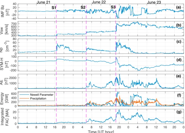
Figure 1. OMNI interplanetary solar wind measurements and the geomagnetic response during the period 21–23 June
2015. The vertical magenta dashed lines (S1, S2, and S3) indicate the time of arrival of the three successive coronal mass ejections that slammed into the Earth. FAC = field-aligned current.
For this study TIE-GCM was run with inputs from the time-dependent high-latitude ionospheric electric potential and auroral precipitation patterns provided by the Assimilative Mapping of Ionospheric Electro-dynamics (AMIE) procedure (see, e.g., Crowley & Hackert, 2001; Richmond, 1992, and references therein). AMIE is an inversion technique driven by data from a diverse array of sources to create a pragmatic rep-resentation of the high-latitude electrodynamic state at a given instance. AMIE can be driven by a range of inputs, including magnetic perturbations from ground-based magnetometers, electric fields computed from ion velocities recorded by radars, digital ionosondes, and satellite observations such as AMPERE (Active Magnetosphere and Planetary Electrodynamics Response) and the Defense Meteorological Satel-lite Program. Other observations that have also been utilized to provide ionospheric conductance inputs for AMIE include particle precipitation data from satellites and UV remote sensing data. From these data, the distribution of different electrodynamic quantities, for example, the electric potential and electric field, height-integrated conductivity, and horizontal and field-aligned currents (FACs) can be determined via electrodynamic equations.
3. Results
3.1. Geomagnetic Disturbance of 22–23 June 2015
On 21–22 June 2015, three successive interplanetary shocks impacted the Earth's magnetosphere (Liu et al., 2015), as marked by the magenta vertical dashed Lines S1, S2, and S3 in Figure 1. The figure exhibits (a) OMNI interplanetary magnetic field (IMF) Bz component, (b) solar wind velocity, (c) solar wind density, (d) SYM-H index, (e) AE index, (f) Newell solar wind coupling function (Newell et al., 2007) and the auroral precipitation calculated from the AE index based on Ostgaard et al. (2002) formulation, and (g) the integrated examined FACs for the Northern Hemisphere derived from AMPERE (Anderson, Takahashi, et al., 2002) on board Iridium spacecraft. The IMF was quite intense having a predominantly southward Bz component from 18:36 to 19:49 UT on 22 June with a storm time peak at ∼19:24 UT reaching a value of −38.9 nT before turning northward suddenly. On 23 June, IMF recorded an extended period of southward Bz between 01:30 and 06:00 UT during which the peak of main phase of the storm occurred. The solar wind speed and density
Figure 2. Time evolution of VTEC (a, c, and e) and storm-to-quiet residual dVTEC (b, d, and f) on 22–23 June. From
top to bottom: 70◦W (American region), 30◦E (European-African) and 120◦E (Asian-Australian). The vertical dotted line represents the time of arrival of Shock S3, while the location of the geomagnetic equator is depicted by the horizontal solid line.
responded strongly to shock S3 with both exhibiting marked jumps. After Shock S3, the speed remained elevated around 600 km/s, while the density steadily decreased to pre-storm levels over a period of about 10-hr. Our major interest for this study is the initial phase immediately after shock S3 at about 18:36 UT on 22 June and the main/recovery phase on 23 June. These periods were associated with intense high-latitude energy injections, multiple TIDs, and large TEC perturbations.
The ring current and high-latitude geomagnetic activity response as portrayed by SYM-H and auroral elec-trojet (AE) indices are shown in Figure 1 (d and e, respectively). After Shock S3, an extreme jump of SYM-H index from −21 to 85 nT (ΔSYM-H =106 nT) was registered, while the AE index, which was already elevated, responded with a sharp increase. The SSC was immediately followed by the rapid growth of the
Journal of Geophysical Research: Space Physics
10.1029/2018JA026172
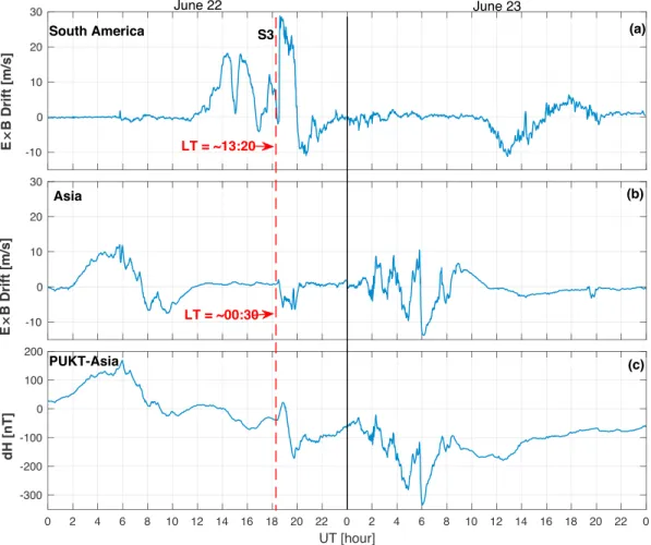
Figure 3. Equatorial electrojet response over South America (a) and Asia (a) during the geomagnetic storm of 22–23
June 2015; dH at a single equator station PUKT (c) is shown for additional verification. Solid black line marks the separation between the 2 days.
storm main phase, which reached a value of −122 nT shortly after 20:00 UT on 22 June. The peak of the main phase occurred at around 04:30 UT on 23 June hitting a minimum SYM-H value of −201 nT (e.g., Astafyeva et al., 2016; Liu et al., 2015; Reiff et al., 2016). Next we examine the solar wind coupling efficiency and the high-latitude energy deposition during the storm (Figure 1f). These parameters are determined using inter-planetary solar wind data (IMF, speed and density) in conjunction with ground-based geomagnetic field measurements. As demonstrated in here, the Newell parameter manifests a sudden large enhancement, which suggests that a highly efficient solar wind-magnetosphere-ionosphere coupling process occurred. Both auroral precipitation and AMPERE FAC (Figure 1g) also sharply responded to shock S3, but we note that similar to AE response, auroral precipitation was already elevated even before S3, which is consistent with AMPERE derived FACs. At the high latitudes, intense TEC was observed around the auroral oval (not shown), which we believe was generated by the intense auroral precipitation.
3.2. Global Ionospheric Response During the June 2015 Storm
As pointed out before, the ionosphere dramatically responded during the June 2015 storm. The present study focuses on the response of the low- and middle-latitude ionosphere. During geomagnetic storms, the EIA crests are sometimes subject to drastic variations and under extreme conditions can significantly expand poleward into the midlatitudes producing the “super fountain effect” (e.g., Astafyeva, 2009; Mannucci et al., 2005; Vlasov et al., 2003). To investigate the global low- and middle-latitude behavior, we focus on VTEC response in three times zones, namely, American (70◦W), European-African (30◦E), and Asian-Australian (120◦E). The evolution of VTEC and storm-to-quiet time residual dVTEC (where dVTEC = storm-day − quiet-day) are revealed in Figure 2. It should be noted that to increase the number of observational points, which was necessary in African and in Asian regions, the cells with zero TEC were filled in with the averaged TEC values from 8 cells around them. In the European-African sector (c and d, nightside) and
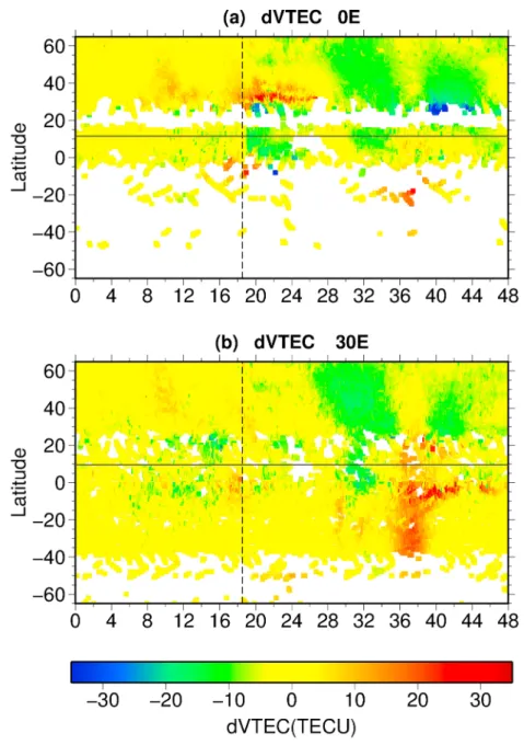
Figure 4. Comparison of residual dVTEC for 0◦E and 30◦E longitudes on 22–23 June 2015. The vertical dotted line represents the time of arrival of Shock S3, while the horizontal solid line represents the geomagnetic equator.
Asian-Australian sector (e and f, postmidnight), TEC generally decreased following the SSC on 22 June and EIA was not formed. Even so, we do note that some enhanced TEC (Figure 2d) is seen around the southern hemisphere in the European-African sector.
On the other hand, a dramatic TEC response was observed in the American sector (Figures 2a and 2b) after SSC. There is a clear asymmetry between the northern and southern EIA with the southern crest appearing to have formed much earlier compared to the northern crest. In fact, a strongly enhanced northern crest fully emerged about 2-hr after shock S3, while the southern crest appears to gradually fade away at the same time. On 23 June, marked positive TEC variations are observed in the Asian-Australian sector (Figure 2f) during the main phase and in the European-Africa sector (Figure 2d) during the recovery phase. These TEC enhancements are observed to last over 6-hr, thus can be classified as long-lasting storm enhanced density (SED) features (e.g., Buonsanto, 1999; Ngwira, McKinnell, Cilliers, & Coster, 2012; Pedatella et al., 2009). The most intense TEC perturbations are observed in the southern winter hemisphere around the southern EIA crest. In contrast to these observations, the American sector (Figure 2b) was characterized by deep TEC
Journal of Geophysical Research: Space Physics
10.1029/2018JA026172
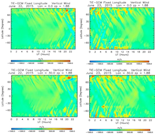
Figure 5. Comparison of simulated vertical winds from the TIE-GCM at fixed longitudes 0◦E and 30◦E. TIE-GCM = Thermosphere-Ionosphere-Electrodynamics General Circulation Model.
depletion during and after the main phase on 23 June. The deepest depletions were registered in the North American region.
The EEJ reaction to the storm in the American and Asian sectors is examined from the equatorial E × B vertical drift data in Figure 3. AMBER (Yizengaw & Moldwin, 2009) and LISN (Valladares & Chau, 2012) data were used to derive the EEJ for American (station pair PUER-LETI, Puerto Maldonado and Leticia) and Asian (BANG-PUKT, Bangkok and Phuket) sectors, respectively, as described in the previous section. Data for the African sector were not available for this period. Figure 3a clearly demonstrates that after Shock S3 the dayside American sector experienced a rapid enhancement of the E×B drift increasing from −3 m/s starting at about 18:36 UT (13:20 LT) to a peak value of 28 m/s at about 18:42 UT (13:26 LT). In contrast, we estimate the nightside current using dH variations at a single geomagnetic equator station, as shown for PUKT in Figure 3c. After the SSC on 22 June, the Asian sector (postmidnight) recorded a sharp-slight increase of dH for a short period, indicating the presence of eastward current, followed by a rapid decrease that is associated with westward current. There is reasonable agreement between the dH and E × B drifts (Figure 3b), thus giving us further confidence in our interpretation of equatorial electrodynamics. Furthermore, the E × B drift variations shown in the present study for both American and Asian sectors are well correlated with C/NOFS vertical plasma drift and SWARM EEJ in situ satellite measurements (see Astafyeva et al., 2018, for comparison).
On 23 June, a decrease of the morning E × B drift (Figure 3a) was registered in the American sector from ∼10:00–16:00 UT (05:00–11:00 LT). In the Asian sector (Figure 3b), daytime E × B drift was characterized by several upward and downward oscillations between 01:00–11:00 UT. These oscillations are considered to be the competing effect between PPEFs and the disturbance dynamo effect (Astafyeva et al., 2018). Downward (negative) drifts can move the ionospheric plasma to lower altitudes where recombination rates are higher resulting in reduced TEC. Perhaps this could explain the strong decrease in TEC observed in the Ameri-can sector (23 June); however, there is no evidence of signifiAmeri-cant TEC changes across the Asian-Australian sector on June 22 and during postmidnight on 23 June, which could be due to competing effect of drivers.
Figure 6. Detrended total magnetic field at two African ground stations on 22–23 June. The yellow shaded area
indicates the specific time of interest when the magnetic field variations at the two stations have large differences.
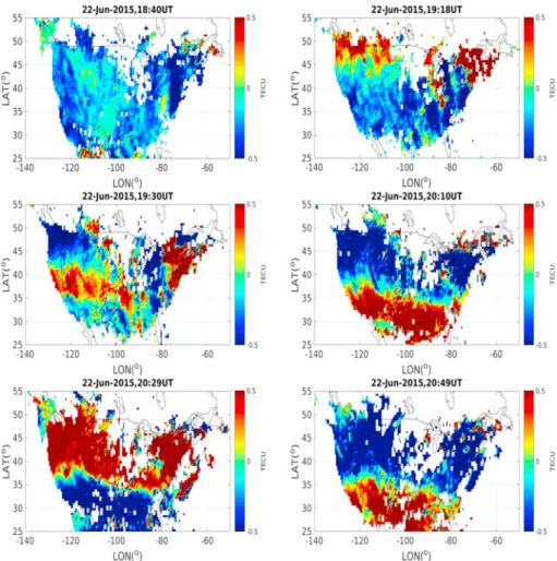
Figure 7. Total electron content perturbation maps showing traveling ionospheric disturbances propagating over North
Journal of Geophysical Research: Space Physics
10.1029/2018JA026172
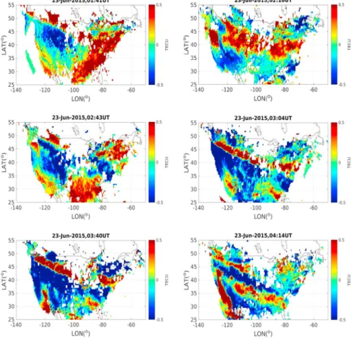
Figure 8. Total electron content perturbation maps showing traveling ionospheric disturbances propagating over North
America at selected time steps during the main phase of the geomagnetic storm on 23 June.
Nevertheless, there was no formation of the EIA during those periods of strong downward drifts in both sectors.
3.3. Longitude and Hemispheric Dependence
In this section, the basis of our investigation are the differences in the longitude and hemispherical response to the storm, specifically targeting the European-African sector. Additional residual dVTEC data in Figure 4 allows us to compare the storm time response at 0◦E and 30◦E. At 0◦E (Figure 4a), there is sparse data in the Southern Hemisphere because it is mostly ocean off the West African coast. Nevertheless, two distinct cases of TEC longitudinal difference are apparent: (1) immediately after arrival of shock S3 on 22 June, and (2) during the recovery phase on 23 June. Furthermore, there is a clear poleward directed enhanced TEC feature at the 30◦E longitude (Figure 4b) starting around 06:00 UT (hour 30) on 23 June that is not as clear for the 0◦E. Also, the intensity of dVTEC (absolute value) along the 0◦latitude related to this enhanced TEC feature is higher in Southern Hemisphere at 30◦E than at 0◦E.
To determine the cause of the TEC variations noted above, we performed a simulation of the storm response using the TIE-GCM model. The TIE-GCM simulated vertical wind patterns for the two sectors are shown in Figure 5. These winds show a very similar response pattern, which suggests that neutral winds could not be the primary cause of the TEC differences but may probably be driven by electric fields. A closer inspection of the detrended total geomagnetic field variations discloses significant differences, as highlighted by the yellow shaded area in Figure 6. Detrending was performed by subtracting the nighttime baseline values of the total magnetic field from the corresponding magnetometer data sets, as discussed in section 2.2. The negative geomagnetic field perturbations at low latitudes are associated with westward current. The largest perturbations are linked to stronger westward currents and downward E × B drifts. Thus, we are confident that the competing effect between electric fields and neutral winds is dominated by electric fields since the wind patterns are relatively similar.
Figure 9. Keograms of total electron content perturbations on (left column) 22 June (18:00–23:59 UT) and (right
column) 23 June (00:00–06:00 UT) in the North America sector. Equatorward large-scale traveling ionospheric disturbances are marked by the dotted arrows. Three longitudinal cuts at 70◦W, 90◦W, and 110◦W are displayed.
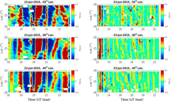
Figure 10. Keograms of total electron content perturbations on (left column) 22 June (18:00–23:59 UT) and (right
column) 23 June (12:00–23:59 UT) in the Brazilian sector. Both equatorward (left column) and poleward (right column) traveling ionospheric disturbances are marked by the dotted arrows. Three longitudinal cuts at 55◦W, 50◦W, and 45◦W are displayed.
Journal of Geophysical Research: Space Physics
10.1029/2018JA026172
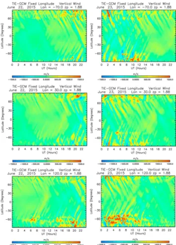
Figure 11. Simulated vertical winds from the TIE-GCM at fixed longitudes 70◦W, 30◦E, and 120◦E. Left column shows 22 June and on the right is 23 June. TIE-GCM = Thermosphere-Ionosphere-Electrodynamics General Circulation Model.
3.4. Equatorward and Poleward Propagating TIDs
Another interesting feature in Figure 2 (b, d, and f) is the manifestation of multiple equatorward and pole-ward extending storm time TEC structures that can be described as TIDs (See supporting information for more analysis). To further analyze the TIDs, 2-D TEC maps are created using the TEC data obtained from our analysis described in section 2.1. The American sector is specifically chosen for this analysis because of the dense GNSS receiver network distribution that allows for the TEC structures to be more clearly mani-fested. The TEC maps are shown in Figures 7 and 8. Both figures display snapshots of TEC perturbations at selected time steps. Large-scale TIDs (or LSTIDs) extending across North America are observed propagating equatorward from the northeast to the southwest direction in both cases. To some extent, LSTIDs typically have long wavelengths that extend to thousands of kilometers, large periods of approximately an hour or more, and traditionally propagate equatorward from high latitudes in either hemisphere.
In order to deduce TID properties such as velocity, wavelength, and period, we construct TEC keogram, as revealed in Figure 9. The keogram images in this study are obtained from the differential TEC derived by using the TID analysis technique described above in section 2.1 The idea is to alternate time variation along fixed longitude and varying latitudes; that is, the differential TEC values were average over range of latitudes and fixed longitude as a function of time for each keogram image. The keograms are constructed for three different longitudes and show elongated TEC structures extending from high to low latitudes. These structures are shifted in time, which implies that they are propagated with time. Based on keogram analysis (see Jonah et al., 2018, for details), TIDs propagate at velocities ranging between 600 and 800 m/s, with a roughly 60-min period and an amplitude of 0.5 TECU. These LSTID properties are consistent with values provided in previous studies (e.g., Coster et al., 2017; Tsugawa et al., 2003; Tsugawa et al., 2004; Zhang et al., 2017). The TIDs observed on 22 June appear to have wavelengths between 1,000 and 3,000 km (Figure 7/ 9), while the TIDs on 23 June have wavelengths between 1,000 and 2,000 km (Figure 8/9).
In addition to equatorward LSTIDs, multiple poleward propagating TIDs that appear to originate at the geo-magnetic equator are also observed in this study. To further probe the presence of poleward TIDs, we also created TEC keograms using data from three Brazilian longitudes shown in Figure 10. The right-side con-tains results for 22 June (18:00–23:59 UT), while the left-side concon-tains results for 23 June (12:00–23:59 UT). Looking at the plots, it is immediately clear that poleward propagating TIDs are present on 23 June but not on 22 June. The poleward TIDs have a wavelength range of 200–500 km and propagate with average velocity of 212 ± 10 m/s and period between 50–90 min. Based on these characteristics, these waves can be classified as medium-scale TIDs (or MSTIDs; Hocke & Schlegel, 1996). Also, it is worth noting that the poleward TIDs were not detected in the North American sector using the same techniques above and during this same time interval. Therefore, we believe that the poleward TIDs did not travel further into the midlatitudes. We suppose that the generation of large-amplitude equatorward propagating TIDs reported in this study is related to enhanced energy injection into the auroral ionosphere. These TIDs are the ionospheric man-ifestation of traveling atmospheric disturbances excited by impulsive auroral processes at high latitudes (Guo et al., 2015; Hines, 1960; Hocke & Schlegel, 1996). During geomagnetic storms, LSTIDs are frequently detected at ionospheric F region heights in the low-middle latitudes. They are induced by low-frequency fast moving traveling atmospheric disturbances with wavelengths of several thousand kilometers that can propagate over large distances. LSTIDs typically tend to exhibit an equatorward meridional propagation from polar regions (Ding et al., 2007; Katamzi & Habarulema, 2013; Ngwira, McKinnell, Cilliers, & Coster, 2012). Our claim on the excitation of these LSTIDs is supported by observations and derived quantities in Figure 1. Furthermore, simulated TIE-GCM model vertical winds in Figure 11 show clear signatures of equa-torward propagating structures initiated at high latitudes in both hemispheres. Several LSTIDs structures are evident but more enhanced vertical winds with velocities in excess of 1,000 m/s are predominately seen at high latitudes after shock S3 at all longitudes on 22 June and also between midnight and 15:00 UT on 23 June. Such high velocities are typical of LSTIDs (Dashora et al., 2009; Habarulema et al., 2016; Ngwira, McKinnell, Cilliers, & Coster, 2012). Interestingly, some of the TID features cross the equator penetrating into the opposite hemisphere (interhemispherical TIDs) in agreement with observations.
4. Discussion and Summary
The arrival of a large CME on 22 June was immediately followed by a major geomagnetic storm. Observa-tions disclose that both positive and negative TEC phases were produced. The TEC decrease can be related to the presence of a downward equatorial E × B drift, as shown in Figure 3. A downward drift is indication of westward electric fields or the equatorial counter EEJ. On the dayside, however, sudden large TEC increases were observed with more than 25 TECU (at selected stations) above the quiet day level representing roughly a 71% increase. For an eastward electric field penetrated to the dayside equator (Figure 3), we expect an increase in the TEC during this interval in the low- and middle-latitude ionosphere (Foster & Rich, 1998; Kelley et al., 2003; Maruyama et al., 2004; Tsurutani et al., 2004).
The trigger for the penetration electric field could perhaps be the sudden reversal of IMF Bz (from +2 to −16 nT in 5 min) at the time of Shock S3, as disclosed in Figure 1. In general, equatorial drifts can be amplified by penetration electric fields of high-latitude origin (Kikuchi et al., 2000). The action of eastward penetration electric fields is to uplift equatorial plasma due to an upward E × B drift so that more plasma is available at higher altitudes where recombination rates are low. This results in a net increase of electron density (or TEC) and an enhanced equatorial fountain effect that explains the development of EIA crests. Furthermore, studies show that the effect of penetration electric field alone in producing enhanced TEC is less than by combining storm-induced equatorward neutral winds and penetration electric fields (Lin et al., 2005). But it must be emphasized that the wind effect is only expected to affect the TEC a few hours after storm commencement if propagation time from high latitudes to equator is taken into account.
On closer inspection of the EIA response (Figure 2), a strong asymmetry between the northern crest and southern crest is clearly evident on 22 June. This asymmetry and development of the EIA was not seen prior to the storm (20 and 21 June), thus implying it was storm induced. Generally, we see a temporally extended EIA crest in the southern (winter) compared to the northern (summer). One of the most striking features in Figure 2 is that the northern EIA crest only develops after shock S3 arrival, while the southern EIA can be seen developing much earlier in the day. The vertical plasma drift plays a big role in the development of the EIA. As discussed above and disclosed in Figure 3, the plasma drift was significantly elevated after Shock S3
Journal of Geophysical Research: Space Physics
10.1029/2018JA026172
but there is also some enhancement just after 1200 UT in the American sector. However, it is well-known that the latitudinal distribution of ionization within the EIA is driven also by thermospheric meridional winds (e.g., Batista et al., 2011; Nogueira et al., 2011, and references therein). A more symmetric EIA implies that a weaker neutral wind effect exists. It is worth noting that the asymmetry can also be due to symmetric winds, that is, transequatorial wind transport from summer to winter hemisphere, as often seen during storms. The June 2015 storm took place at solstice conditions, when the background thermospheric winds on the dayside are strong and directed from summer to winter (Fuller-Rowell et al., 1996). This asymmetry in the neutral winds could explain the asymmetry several hours before the storm.
The high-latitude source of equatorward propagating LSTIDs shown here is clearly related to enhanced storm time neutral winds triggered by large energy deposition in the auroral ionosphere. However, the ini-tiation process of poleward propagating TIDs originating at the dip equator is not quite clear. For instance, Habarulema et al. (2016) suggest that changes in E×B vertical drift after the storm onset could be the source of poleward propagating TIDs, but on the other hand, the poleaward TIDs in the American sectors don't show any correlation with changes in E × B drift. Furthermore, it is worth noting that the TIE-GCM model evidently captures equatorward LSTIDs, including their interhemispherical propagation, but does not repro-duce the poleward propagating MSTIDs of equatorial origins at all. So then, what could be driving these poleward TIDs? What components or physics is missing in the TIE-GCM model? Or are we seeing cases of interhemispherical TIDs amplified as the cross the geomagnetic equator? As pointed out in section 2.3, we used the standard TIE-GCM model settings, which do not include tidal forcing that is important for cou-pling of the ionosphere to the lower atmosphere. Perhaps this could explain why the model is not able to reproduce the poleward propagating MSTIDs.
Regardless of the results shown here, poleward MSTIDs have generally not been extensively studied as compared to their equatorward counterparts that are a common feature during geomagnetic storms. How-ever, there has been a growing number of studies that identify these poleward TIDs (e.g., Ding et al., 2013; Habarulema et al., 2015; Habarulema et al., 2017; Jonah et al., 2018; Zakharenkova et al., 2016, and refer-ences therein). The excitation mechanism(s) for the poleward MSTIDs is still under debate, to the best of our knowledge, but some studies suggest that those events originating at the dip equator during storms are likely related to increased Lorentz coupling due to changes in EEJ (Habarulema et al., 2015; Habarulema et al., 2017). Other studies suggest that poleward TIDs could be produced via deep convection induced by atmospheric gravity waves generated from tropospheric weather (e.g., Jonah et al., 2018). The implication of this mixed-result scenario is that poleward propagating TIDs could be excited/driven by a variety of physical processes that could not be identified in this study, such as tropospheric or mesospheric sources (e.g., Ding et al., 2013; Jonah et al., 2018; Vadas & Liu, 2009; Vadas & Crwoley, 2010; Valladares & Hei, 2012). At present we do not have enough information to full address the questions above, Therefore, more in-depth studies are required to explore the drivers of poleward propagating MSTIDs, including modifying specification of inputs and coupling in the TIE-GCM simulation environment.
References
Anderson, D., Anghel, A., Chau, J., & Veliz, O. (2004). Daytime vertical E×B drift velocities inferred from ground-based magnetometer observations at low latitudes. Space Weather, 2, S11001. https://doi.org/10.1029/2004SW000095
Anderson, D., Anghel, A., Yumoto, K., Ishitsuka, M., & Kudeki, E. (2002). Estimating daytime vertical E×B drift velocities in the equa-torial F-region using ground-based magnetometer observations. Geophysical Research Letters, 29(12), 1596. https://doi.org/10.1029/ 2001GL014562
Anderson, D., Araujo-Pradere, E., & Scherliess, L. (2009). Comparing daytime, equatorial E×B drift velocities and TOPEX/TEC obser-vations associated with the 4-cell, non-migrating tidal structures. Annales Geophysicae, 27, 2861–2867. https://doi.org/10.5194/ angeo-27-2861-2009
Anderson, B. J., Takahashi, K., Kamei, T., Waters, C. L., & Toth, B. A. (2002). Birkeland current system key parameters derived from Iridium observations: Method and initial validation results. Journal of Geophysical Research, 107(A6), 1079. https://doi.org/10.1029/ 2001JA000080
Appleton, E. V. (1946). Two anomalies in the ionosphere. Nature, 157, 691.
Astafyeva, E. (2009). Dayside ionospheric uplift during strong geomagnetic storms as detected by the CHAMP, SAC-C, TOPEX and Jason-1 satellites. Advances in Space Research, 43, 1749–1756. https://doi.org/10.1016/j.asr.2008.09.036
Astafyeva, E., Zakharenkova, I., & Alken, P. (2016). Prompt penetration electric fields and the extreme topside ionospheric response to the June 22–23, 2015 geomagnetic storm as seen by the Swarm constellation. Earth, Planets and Spaces, 68, 152. https://doi.org/10.1186/ s40623-016-0526-x
Astafyeva, E., Zakharenkova, I., Hozumi, K., Alken, P., Co˙Isson, P., Hairston, M. R., & Coley, W. R. (2018). Study of the equatorial and Low-Latitude electrodynamic and ionospheric disturbances during the 22–23 June 2015 geomagnetic storm using ground-based and spaceborne techniques. Journal of Geophysical Research: Space Physics, 123, 2424–2440. https://doi.org/10.1002/2017JA024981
Acknowledgments
Anthea Coster and Evan Thomas are acknowledged for their support to this study. The authors thank M. B. Moldwin, C. E Valladares, and the rest of the AMBER and LISN teams for the equatorial magnetometer data. AMBER is operated by Boston College with funding from NASA and AFOSR. LISN is a project led by the University of Texas at Dallas in collaboration with the Geophysical Institute of Peru and other institutions that provide information for the benefit of the scientific community. Their data are available from http://lisn.igp.gob.pe website. We thank the NSF-funded CEDAR OpenMadrigal web service http://cedar.openmadrigal.org for the VTEC data used in this work. OMNI solar wind data are publicly available via the NASA Goddard Space Flight Center Space Physics Data Facility (http://cdaweb.gsfc.nasa.gov/). We thank the AMPERE team and the AMPERE Science Center for providing the Iridium-derived data products. The results presented in this paper rely on data collected at magnetic
observatories. We thank the national institutes that support them and INTERMAGNET for promoting high standards of magnetic observatory practice www.intermagnet.org. Research at ASTRA and the Catholic University of America is supported by NSF CEDAR Grant AGS-1651268. J. B. H.'s work was partially supported by funding Grant 112090 from the South African National Research Foundation. O. F. Jonah acknowledge support from NASA LWS grant NNX15AB83G. The authors thank the anonymous reviewers for their assistance in evaluating this paper.
Astafyeva, E., Zakharenkova, I., Huba, J. D., Doornbos, E., & van den IJssel, J. (2017). Global ionospheric and thermospheric effects of the geomagnetic disturbances: Multi-instrumental observations and modeling. Journal of Geophysical Research: Space Physics, 122, 11,716–11,742. https://doi.org/10.1002/2017JA024174
Aydogdu, M. (1988). North-south asymmetry in the ionospheric equatorial anomaly in the African and the west Asian regions pro-duced by asymmetrical thermospheric winds. Journal of Atmospheric and Terrestrial Physics, 50(7), 623–627. https://doi.org/10.1016/ 0021-9169(88)90060-8
Baker, D. N., Jaynes, A. N., Turner, D. L., Nakamura, R., Schmid, D., Mauk, B. H., et al. (2016). A telescopic and microscopic examination of acceleration in the June 2015 geomagnetic storm: Magnetospheric Multiscale and Van Allen Probes study of substorm particle injection.
Geophysical Research Letters, 43, 6051–6059. https://doi.org/10.1002/2016GL069643
Batista, I. S., Diogo, E. M., Souza, J. R., Adbu, M. A., & Bailey, G. J. (2011). https://doi.org/10.1007/978-94-007-0326-1&urluscore;23 Buonsanto, M. J. (1999). Ionospheric storms—A review. Space Science Reviews, 88, 563–601.
Chandra, H., & Rastogi, R. G. (1974). Geomagnetic storm effects on ionospheric drifts and the equatorial Es over the magnetic equator.
Indian Journal of Radio and Space Physics, 3, 332–336.
Cherniak, I., & Zakaharenkova, I. (2016). First observations of super plasma bubbles in Europe. Geophysical Research Letters, 43, 11,137–11,145. https://doi.org/10.1002/2016GL071421
Coster, A. J., Goncharenko, L., Zhang, S.-R., Erickson, P. J., Rideout, W., & Vierinen, J. (2017). GNSS Observations of ionospheric variations during the 21 August 2017 solar eclipse. Geophysical Research Letters, 44, 12,041–12,048. https://doi.org/10.1002/2017GL075774 Crowley, G., Emery, B. A., Roble, R. G., Carlson, H. C., & Knipp, D. J. (1989). Thermospheric dynamics during the equinox transition study
I. Model simulations for September 18 and 19, 1984. Journal of Geophysical Research, 94, 16,925–16,944.
Crowley, G., Emery, B. A., Roble, R. G., Carlson, H. C., Salah, J. E., Wickwar, V. B., et al. (1989). Thermospheric dynamics during the equinox transition study of September 1994 II. Validation of the NCAR-TGCM. Journal of Geophysical Research, 94, 16,945–16,960. Crowley, G., & Hackert, C. L. (2001). Quantification of high latitude electric field variability. Geophysical Research Letters, 28(14),
2783–2786. https://doi.org/10.1029/2000GL012624
Crowley, G., Knipp, D. J., Drake, K. A., Lei, J., Sutton, E., & Lu̇hr, H. (2010). Thermospheric density enhancements in the dayside cusp region during strong Byconditions. Geophysical Research Letters, 37, L07110. https://doi.org/10.1029/2009GL042143
Dashora, N., Sharma, S., Dabas, R. S., Alex, S., & Pandey, R. (2009). Large enhancements in low latitude total electron content during 15 May 2005 geomagnetic storm in Indian zone. Annales Geophysicae, 27, 1802–1820.
de Siqueira, P. M., de Paula, E. R., Muella, M. T. A. H., Rezende, L. F. C., Abdu, M. A., & Gonzalez, W. D. (2011). Storm-time total electron content and its response to penetration electric fields over South America. Annales Geophysicae, 29, 1765–1778.
Ding, F., Wan, W., Ning, B., & Wang, M. (2007). Large-scale traveling ionospheric disturbances observed by GPS total electron content during the magnetic storm of 29–30 October 2003. Journal of Geophysical Research, 112, A06309. https://doi.org/10.1029/2006JA012013 Ding, F., Wan, W., Ning, B., Zhao, B., Li, Q., Wang, Y., et al. (2013). Observations of poleward-propagating large-scale traveling Discussions
ionospheric disturbances in southern China. Annales Geophysicae, 31, 377–385. https://doi.org/10.5194/angeo-31-377-2013 Foster, J. C. (1993). Storm time plasma transport at middle and high latitude. Journal of Geophysical Research, 98(A2), 1675–1689. Foster, J. C., & Rich, F. J. (1998). Prompt midlatitude electric fields effects during severe geomagnetic storms. Journal of Geophysical
Research, 103(A11), 26,367–26,372.
Fuller-Rowell, T. J., Codrescu, M. V., Rishbeth, H., Moffett, R. J., & Quegan, S. (1996). Seasonal response of the thermosphere and ionosphere to geomagnetic storms. Journal of Geophysical Research, 101, 2343–2353.
Goodman, J. M. (2005). Operational communication systems and relationships to the ionosphere and Space Weather. Advances in Space
Research, 36(12), 2241–2252.
Guo, J., Forbes, J. M., Wei, F., Feng, X., Liu, H., Wan, W., et al. (2015). Observations of a large-scale gravity wave propagating over an extremely large horizontal distance in the thermosphere. Geophysical Research Letters, 6560–6565. https://doi.org/10.1002/ 2015GL065671
Habarulema, J. B., Katamzi, Z. T., & Yizengaw, E. (2015). First observations of poleward large-scale traveling ionospheric disturbances over the african sector during geomagnetic storm conditions. Journal of Geophysical Research: Space Physics, 120, 6914–6929. https://doi.org/ 10.1002/2015JA021066
Habarulema, J. B., Katamzi, Z. T., Yizengaw, E., Yamazaki, Y., & Seemala, G. (2016). Simultaneous storm time equatorward and poleward large-scale TIDs on a global scale. Geophysical Research Letters, 43, 6678–6686. https://doi.org/10.1002/2016GL069740
Habarulema, J. B., Yizengaw, E., Katamzi, Z. T., Moldwin, M. B., & Buchert, S. (2017). Storm time global observations of large-scale TIDs from ground-based and in situ satellite measurements. Journal of Geophysical Research: Space Physics, 123, 711–724. https://doi.org/10. 1002/2017JA024510
Hines, C. O. (1960). Internal atmospheric gravity waves at ionospheric heights. Canadian Journal of Physics, 38, 1441–1481.
Hocke, K., & Schlegel, K. (1996). A review of atmospheric gravity waves and traveling ionospheric disturbances. Annales Geophysicae, 14, 917–940.
Jonah, O. F., Coster, A., Zhang, L. G. S., Erickson, P. J., de Paula, E. R., & Kherani, E. A. (2018). TID Observations and source analysis during the 2017 memorial day weekend geomagnetic storm over North America. Journal of Geophysical Research: Space Physics, 123, 8749–8765. https://doi.org/10.1029/2018JA025367
Jonah, O. F., Kherani, E. A., & de Paula, E. R. (2016). Observation of TEC perturbation associated with mediumscale traveling ionospheric disturbance and possible seeding mechanism of atmospheric gravity wave at a Brazilian sector. Journal of Geophysical Research: Space
Physics, 121, 2531–2546. https://doi.org/10.1002/2015JA022273
Jones, Jr. M., Forbes, J. M., Hagan, M. E., & Maute, A. (2014). Impacts of vertically propagating tides on the mean state of the ionosphere-thermosphere system. Journal of Geophysical Research: Space Physics, 119, 2197–2213. https://doi.org/10.1002/ 2013JA019744
Katamzi, Z. T., & Habarulema, J. B. (2013). Traveling ionospheric disturbances observed at South African midlatitudes during the 29–31 October 2003 geomagnetically disturbed period. Advances in Space Research, 53, 48–62. https://doi.org/10.1016/j.asr.2013.10.019 Kelley, M. C., Makela, J. J., Chau, J. L., & Nicolls, M. J. (2003). Penetration of the solar wind electric field into the magnetosphere/ionosphere
system. Geophysical Research Letters, 30(4), 1158. https://doi.org/10.1029/2002GL016321
Kikuchi, T., Lu̇ehr, H., Schlegel, K., Tachihara, H., Shinohara, M., & Kitamura, T.-I. (2000). Penetration of auroral electric fields to the equator during a substorm. Journal of Geophysical Research, 105, A10.
Kuai, J., Liu, L., Liu, J., Zhao, B., Chen, Y., Le, H., & Wan, W. (2015). The long-duration positive storm effects in the equatorial ionosphere over Jicamarca. Journal of Geophysical Research: Space Physics, 120, 1311–1324. https://doi.org/10.1002/2014JA020552
Journal of Geophysical Research: Space Physics
10.1029/2018JA026172
Lin, C. H., Richmond, A. D., Heelis, R. A., Bailey, G. J., Lu, G., Liu, J. Y., et al. (2005). Theoretical study of the low- and midlatitude ionospheric electron density enhancement during the October 2003 superstorm: Relative importance of the neutral wind and electric field. Journal of Geophysical Research, 110, A12312. https://doi.org/10.1029/2005JA011304
Liu, J. D., Hu, H., Wang, R., Yang, Z., Zhu, B., Liu, Y. A., et al. (2015). Plasma and magnetic field characteristics of solar coronal mass ejections in relation to geomagnetic storm intensity and variability. Astrophysical Journal Letters. arXiv:1508.01267v1 [physics.space-ph, 10.1088/2041-8205/809/2/L34.
Luo, W., Zhu, Z., Xiong, C., & Chang, S. (2017). The response of equatorial ionization anomaly in 120◦E to the geomagnetic storm of 18 August 2003 at different altitudes from multiple satellite observations. Space Weather, 15, 1588–1601. https://doi.org/10.1002/ 2017SW001710
Mannucci, A. J., Tsurutani, B. T., Iijima, B. A., Komjathy, A., Saito, A., Gonzalez, W. D., et al. (2005). Dayside global ionospheric response to the major interplanetary events of October 29–30, 2003 “Halloween Storms”. Geophysical Research Letters, 32, L12S02. https://doi. org/10.1029/2004GL021467
Maruyama, T., Ma, G., & Nakamura, M. (2004). Signature of TEC storm on 6 November 2001 derived from dense GPS receiver network and ionosonde chain over Japan. Journal of Geophysical Research, 109, A10302. https://doi.org/10.1029/2004JA010451
Mendillo, M. (2006). Storms in the ionosphere: Patterns and processes for total electron content. Reviews of Geophysics, 44, RG4001. https:// doi.org/2005RG000193
Nakamura, R., Sergeev, V. A., Baumjohann, W., Plaschke, F., Magnes, W., Fischer, D., et al. (2016). Transient, small-scale field-aligned currents in the plasma sheet boundary layer during storm time substorms. Geophysical Research Letters, 43, 4841–4849. https://doi.org/ 10.1002/2016GL068768
Newell, P. T., Sotirelis, T., Liou, K., Meng, C.-I., & Rich, F. J. (2007). A nearly universal solar wind-magnetosphere coupling function inferred from 10 magnetospheric state variables. Journal of Geophysical Research, 112, A01206. https://doi.org/10.1029/2006JA012015 Ngwira, C. M., & Coster, A. (2017). Global ionospheric electron density disturbances during the initial phase of a geomagnetic storm on
April 5, 2010. In T. Fuller-Rowell, E. Yizengaw, P. H. Doherty, & S. Basu (Eds.), In ionospheric space weather: Longitude and hemispheric
dependences and lower atmosphere forcing(Vol. 220, pp. 257–279). https://doi.org/10.1002/978111892916.ch21
Ngwira, C. M., McKinnell, L. A., Cilliers, P. J., & Coster, A. J. (2012). Ionospheric observations during the geomagnetic storm events on 24–27 July 2004: Long-duration positive storm effects. Journal of Geophysical Research, 117, A00L02. https://doi.org/10.1029/ 2011JA016990
Ngwira, C. M., McKinnell, L. A., Cilliers, P. J., & Yizengaw, E. (2012). An investigation of ionospheric disturbances over South Africa during the magnetic storm on 15 May 2005. Advances in Space Research, 49, 327–335. https://doi.org/10.1016/j.asr.2011.09.035
Nogueira, P. A. B., Adbu, M. A., Batista, I. S., & de Siqueira, P. M. (2011). Equatorial ionization anomaly and thermospheric meridional winds during two major storms over Brazilian low latitudes. Journal of Atmospheric and Solar–Terrestrial Physics, 73, 1535–1543. https:// doi.org/10.1016/j.jastp.2011.02.008
Ostgaard, N., Germany, G., Stadnes, J., & Vondrak, R. R. (2002). Energy analysis of substorms based on remote sensing techniques, solar wind measurements, and geomagnetic indices. Journal of Geophysical Research, 107(A9), 1233. https://doi.org/10.1029/2001JA002002 Pedatella, N. M., Lei, J., Larson, K. M., & Forbes, J. M. (2009). Observations of the ionospheric response to the 15 December 2006
geomag-netic storm: Long-duration positive storm effect. Geophysical Research Letters, 114, A12313. https://doi.org/10.1029/2009JA014568 Reiff, P. H., Daou, A. G., Sazykin, S. Y., Nakamura, R., Hairston, M. R., Coffey, V., et al. (2016). Multispacecraft observations and modeling
of the 22/23 June 2015 geomagnetic storm. Geophysical Research Letters, 43, 7311–7318. https://doi.org/10.1002/2016GL069154 Richmond, A. D. (1992). Assimilative mapping of ionospheric electrodynamics. Advances in Space Research, 12(6), 659–668. Rideout, W., & Coster, A. (2006). Automated GPS, processing for global total electron content data. GPS Solutions, 10(3), 219–228. Savitzky, A., & Golay, M. J. E. (1964). Smoothing and differentiation of data by simplified Least-Squares procedures. Analytical Chemistry,
36, 1627–1639. https://doi.org/10.1021/ac60214a047
Singh, R., & Sripathi, S. (2017). Ionospheric response to 22–23 June 2015 storm as investigated using Ground-Based ionosondes and GPS receivers over India. Journal of Geophysical Research: Space Physics, 122, 11,645–11,664. https://doi.org/10.1002/2017JA024460 Tsugawa, T., Saito, A., & Otsuka, Y. (2004). A statistical study of large-scale travelling ionospheric disturbances using the GPS network in
Japan. Journal of Geophysical Research, 109, A06302. https://doi.org/10.1029/2003JA010302
Tsugawa, T., Saito, A., Otsuka, Y., & Yamamoto, M. (2003). Damping of large-scale traveling ionospheric disturbances detected with GPS networks during the geomagnetic storm. Journal of Geophysical Research, 108(A3), 1127. https://doi.org/10.1029/2002JA009433 Tsurutani, B., Mannucci, A., Iijima, B., Abdu, M. A., Humberto, J., Sobral, A., et al. (2004). Global dayside ionospheric uplift and
enhancement associated with interplanetary electric fields. Journal of Geophysical Research, 109, A08302. https://doi.org/10.1029/ 2003JA010342
Vadas, S. L., & Crwoley, G. (2010). Sources of the traveling ionospheric disturbances observed by the ionospheric TIDDBIT sounder near Wallops Island on 30 October 2007. Journal of Geophysical Research, 115, A07324. https://doi.org/10.1029/2009JA015053
Vadas, S. L., & Liu, H. (2009). Generation of large-scale gravity waves and neutral winds in the thermosphere from the dissipation of convectively generated gravity waves. Journal of Geophysical Research, 114, A10310. https://doi.org/10.1029/2009JA014108
Valladares, C. E., & Chau, J. L. (2012). The low-latitude ionosphere sensor network: Initial results. Radio Science, 47, RS0L17. https://doi. org/10.1029/2011RS004978
Valladares, C. E., & Hei, M. A. (2012). Measurement of the characteristics of TIDs using small and regional networks of GPS receivers during the campaign of 17–30 July of 2008. International Journal of Geophysics, 2012, 548784. https://doi.org/10.1155/2012/548784 Vierinen, J., Coster, A. J., Rideout, W. C., Erickson, P. J., & Norberg, J. (2016). Statistical framework for estimating GNSS bias. Atmospheric
Measurement Techniques, 9(3), 1303–1312. https://doi.org/10.5194/amt-9-1303-2016
Vlasov, M., Kelley, M. C., & Kil, H. (2003). Analysis of ground-based and satellite observations of F,-region behavior during the great magnetic storm of July 15, 2000. Journal of Atmospheric and Solar-Terrestrial Physics, 65, 1223–1234.
Yizengaw, E., Dewar, J., MacNeil, J., Moldwin, M. B., Galvan, D., Sanny, J., et al. (2008). The occurrence of ionospheric signatures of plasmaspheric plumes over different longitudinal sectors. Journal of Geophysical Research, 113, A08318. https://doi.org/10.1029/ 2007JA012925
Yizengaw, E., & Moldwin, M. B. (2009). African Meridian B-field Education and Research (AMBER) Array. Earth Moon Planet, 104(1), 237–246. https://doi.org/10.1007/s11038-008-9287-2
Yizengaw, E., Moldwin, M. B., Dyson, P. L., & Immel, T. J. (2005). Southern Hemisphere ionosphere and plasmasphere response to the interplanetary shock event of 29-31 October 2003. Journal of Geophysical Research, 110, A09S30. https://doi.org/10.1029/2004JA010920 Yizengaw, E., Moldwin, M. B., Mebrahtu, A., Damtie, B., Zesta, E., Valladares, C. E., & Doherty, P. (2011). Comparison of storm time equatorial ionospheric electrodynamics in the African and American sectors. Journal of Atmospheric and Solar-Terrestrial Physics, 73(1), 156–163. https://doi.org/10.1016/j.jastp.2010.08.008
Yizengaw, E., Moldwin, M. B., Zesta, E., Biouele, C. M., Damtie, B., Mebrahtu, M., et al. (2014). The longitudinal variability of equatorial electrojet and vertical drift velocity in the african and american sectors. Annales of Geophysicae, 32, 231–238. https://doi.org/10.5194/ angeo-32-231-2014
Zakharenkova, I., Astafyeva, E., & Cherniak, I. (2016). GPS And GLONASS observations of traveling ionospheric disturbances during the 2015 St. Patrick's Day storm. Journal of Geophysical Research: Space Physics, 121, 12,138–12,156. https://doi.org/10.1002/2016JA023332 Zhang, S., Erickson, P. J., Goncharenko, L., Coster, A. J., Rideout, W., & Vierinen, J. (2017). Ionospheric bow waves and perturbations induced by the 21 August 2017 solar eclipse. Geophysical Research Letters, 44, 12,067–12,073. https://doi.org/10.1002/2017GL076054 Zhao, B., Wan, W., & Liu, L. (2005). Responses of equatorial anomaly to the October–November 2003 superstorms. Annales of Geophysicae,