Geophysical validation of SCIAMACHY Limb Ozone Profiles

HAL Id: hal-00328416

https://hal.archives-ouvertes.fr/hal-00328416

Submitted on 26 Jan 2006

HAL is a multi-disciplinary open access

archive for the deposit and dissemination of

sci-entific research documents, whether they are

pub-lished or not. The documents may come from

teaching and research institutions in France or

abroad, or from public or private research centers.

L’archive ouverte pluridisciplinaire HAL, est

destinée au dépôt et à la diffusion de documents

scientifiques de niveau recherche, publiés ou non,

émanant des établissements d’enseignement et de

recherche français ou étrangers, des laboratoires

publics ou privés.

Profiles

E. J. Brinksma, A. Bracher, D. E. Lolkema, A. J. Segers, I. S. Boyd, K.

Bramstedt, H. Claude, Sophie Godin-Beekmann, G. Hansen, G. Kopp, et al.

To cite this version:

E. J. Brinksma, A. Bracher, D. E. Lolkema, A. J. Segers, I. S. Boyd, et al.. Geophysical validation

of SCIAMACHY Limb Ozone Profiles. Atmospheric Chemistry and Physics, European Geosciences

Union, 2006, 6 (1), pp.209. �hal-00328416�

www.atmos-chem-phys.org/acp/6/197/ SRef-ID: 1680-7324/acp/2006-6-197 European Geosciences Union

Chemistry

and Physics

Geophysical validation of SCIAMACHY Limb Ozone Profiles

S. Godin-Beekmann6, G. Hansen7, G. Kopp8, T. Leblanc9, I. S. McDermid9, Y. J. Meijer3, H. Nakane10, A. Parrish11, C. von Savigny2, K. Stebel7, D. P. J. Swart3, G. Taha12,13, and A. J. M. Piters1

1_{KNMI, Postbus 201, 3730 AE De Bilt, The Netherlands}

2_{Institute of Environmental Physics (IFE), University of Bremen, PO Box 330440, 28334 Bremen, Germany} 3_{National Institute for Public Health and the Environment (RIVM), Bilthoven, The Netherlands}

4_{NIWA, Environmental Research Institute, Ann-Arbor, MI 48108, USA}

5_{Deutscher Wetterdienst, Meteorologisches Observatorium, Albin SchwaigerWeg 10, 82383 Hohenpeissenberg, Germany} 6_{Service d’A´eronomie – CNRS, Institut Pierre Simon Laplace, 4 Place Jussieu, 75252 Paris Cedex 05, France}

7_{Norwegian Institute for Air Research (NILU), Polar Environmental Centre, Tromsoe, Norway} 8_{IMK, Forschungszentrum Karlsruhe and Universit¨at Karlsruhe, Germany}

9_{NASA-JPL, Wrightwood (CA) USA}

10_{Atmospheric Environment Division, National Institute for Environmental Studies, 16-2, Onogawa, Tsukuba, Ibaraki}

305-8506, Japan

11_{University of Massachusetts, USA}

12_{Science and Application International Corporation, Hampton (VA), USA} 13_{NASA-Langley Research Center, MS 475, Hampton (VA), 23681, USA}

Received: 6 April 2005 – Published in Atmos. Chem. Phys. Discuss.: 14 July 2005 Revised: 20 December 2005 – Accepted: 6 January 2006 – Published: 26 January 2006

Abstract. We discuss the quality of the two available

SCIA-MACHY limb ozone profile products. They were retrieved with the University of Bremen IFE’s algorithm version 1.61 (hereafter IFE), and the official ESA offline algorithm (here-after OL) versions 2.4 and 2.5. The ozone profiles were com-pared to a suite of correlative measurements from ground-based lidar and microwave, sondes, SAGE II and SAGE III (Stratospheric Aerosol and Gas Experiment).

To correct for the expected Envisat pointing errors, which have not been corrected implicitly in either of the algorithms, we applied a constant altitude shift of −1.5 km to the SCIA-MACHY ozone profiles.

The IFE ozone profile data between 16 and 40 km are bi-ased low by 3–6%. The average difference profiles have a typical standard deviation of 10% between 20 and 35 km.

We show that more than 20% of the SCIAMACHY offi-cial ESA offline (OL) ozone profiles version 2.4 and 2.5 have unrealistic ozone values, most of these are north of 15◦S. The remaining OL profiles compare well to correlative in-struments above 24 km. Between 20 and 24 km, they under-estimate ozone by 15±5%.

Correspondence to: A. J. M. Piters

(piters@knmi.nl)

1 Introduction

SCIAMACHY (SCanning Imaging Absorption spectroMe-ter for Atmospheric CartograpHY) is a limb and nadir mode viewing satellite instrument, which also has the possibil-ity to do occultation measurements, that measures the Earth reflectance between 240 and 2380 nm (Bovensmann et al., 1999).

In the limb mode, horizontal scans of the Earth’s atmo-sphere from about −3 to +92 km are made, with 3.3 km ver-tical intervals. Thirteen of these scans are used for ozone profile retrieval.

Two SCIAMACHY limb ozone profile products are cur-rently available, both are discussed in this paper. Retrievals have been developed by these two groups: The Institute for Environmental Physics in Bremen (IFE), who developed an unofficial SCIAMACHY product (often referred to as “scien-tific product” within the SCIAMACHY community) and the DLR in Oberpfaffenhofen, who developed the official ESA offline algorithm.

The retrieved ozone profile is a smoothed version of the true profile. The smoothing is described by the averaging kernel matrix in combination with the a priori profile, in the sense that every element of the retrieved profile is the a priori value plus a weighted average of differences between true and a priori at several heights.

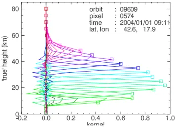
Fig. 1. Example of averaging kernels used in the IFE1.61 ozone

profile retrievals (mid latitude, 1 January, for details see legend within the figure). The averaging kernels are defined on a fixed vertical grid with resolution of about 3 km up to 50 km, and 5 km above.

Figure 1 shows an example of the averaging kernels for the IFE product. Evidently, the limb retrieval has a high vertical resolution (sharp averaging kernels), especially around the ozone maximum at approximately 20 km.

The squares in Fig. 1 show the altitude assignment of each of the elements in the ozone profile. Between 15 and 45 km the kernels peak at the assigned altitude of a profile element. SCIAMACHY is insensitive to ozone below 12 km, which is reflected in the averaging kernel shapes in Fig. 1. The IFE retrieval takes into account some layers below that altitude in order to obtain smooth tropospheric profiles. This is evi-dently not measurement information.

IFE limb ozone profile retrievals are based on the Chap-puis bands of ozone (von Savigny et al., 2005a), which are in the visible wavelengths. Retrievals are performed from SCIAMACHY level 0 files using the SCIARAYS radiative transfer model (Kaiser, 2001). One ozone profile per SCIA-MACHY state is retrieved, in units of number density against altitude. Averaging kernels are provided. For the a priori pro-files, the SBUV climatology (McPeters, 1993) is used.

ESA offline DLR retrievals (hereafter OL) are based on ozone absorption exclusively in the ultraviolet window of 319–333 nm. Four ozone profiles per state are retrieved. The available data consist of the 2002 data described in Brinksma et al. (2004), and two recent subsets: data be-tween 20 September 2004 and 27 November 2004 (hereafter OL2.4) and data from 7 December 2004 and onward (in this paper through 17 February, hereafter OL2.5). Although the version numbers differ, the processor and all inputs relevant for ozone profile retrievals were identical (S. Hilgers, DLR, personal communication, 2005). These data are relatively re-cent at the time of writing, hence the number of collocations with ground and balloon instruments is limited, because for many locations, data were not yet available in databases. For

the OL data sets, we will only consider the ozone profiles in units of number density (which we derive from the listed partial columns) against altitude. Averaging kernels for the offline algorithm are not contained in the product or publicly available.

In an earlier paper, validation of the offline algorithm ver-sion 2.1 applied to the validation reference data set (383 se-lected SCIAMACHY limb states from 18 July through 16 December 2002), and the IFE algorithm version 1.6, applied to available level 0 states between July and December 2002 was discussed based on comparisons to correlative instru-ments (Brinksma et al., 2004). Conclusions were that the OL2.1 as well as IFE1.6 profiles agreed within about 10% for the 20–40 km region when compared with groundbased data, and within about 20% when compared with satellite data. However, the standard deviations on the differences be-tween SCIAMACHY and correlative instruments were rather large (10–40%). The results were dominated by uncertainties in the altitude assignment, caused by Envisat pointing inac-curacies, which are discussed in Sect. 2. Another problem was that the data set was too small to get good statistics. In the current paper, we present the status of the most recent algorithm versions, based on recent SCIAMACHY measure-ments in which the pointing problem should be less.

A number of more recent validation studies on IFE version 1.6 have been performed. Bracher et al. (2005) compared IFE1.6 data from October and November 2003 with MIPAS-IMK and GOMOS-ACRI data products. The three retrievals mutually agreed within 15% between 22 and 38 km. Com-parisons with ozone sondes by Segers et al. (2005) show that IFE1.6 and sondes differ 10–15% in the 10–30 km range, after application of an overal shift of 2 km to cor-rect for the pointing error. The analysed period is August– December 2002. They also showed that the gradients in ozone (below as well as above the ozone number density maximum) were too steep. Palm et al. (2005) compared IFE1.6 data between August 2002 and August 2003 with two microwave radiometers in Bremen and Ny- ˚Alesund and concluded that they agree within the expected covariance of the intercomparison, after shifting the SCIAMACHY pro-files downward with 1.5 km. A preliminary comparison with FTIR for only a few collocations showed large devia-tions, especially below 20 km. Comparisons of IFE1.6 data with ASUR measurements for 11 flights in September 2002, February 2003 and March 2003 (Kuttipurath et al., 2004) re-sult in deviations ranging from −12 to +15% between 20 and 40 km, after subtraction of a constant positive bias of 12% in the ASUR data. The pointing error in this study was ac-counted for by applying a retrieved tangent height error fol-lowing Kaiser et al. (2004). De Clercq et al. (2004) compared IFE1.6 data between July and December 2002 with measure-ments from ozone sondes, lidars and microwave radiome-ters. Deviations between 18 and 40 km range from −30% to +30%, which is mainly caused by Envisat’s altitude regis-tration error (see Sect. 2).

Recently, data processed with a newer algorithm, namely IFE version 1.61, have become available. Since these data are considerably different from the previous version, we will limit the discussion to version 1.61 only. The validated data set consists of five months of data (all available orbits during January, March, May, September, and November 2004).

2 Envisat pointing

A study of the Envisat pointing accuracy showed that differ-ences of up to 3 km were found between the on-board orbit propagator and the retrieved pointing (from the UV limb ra-diances) for the period up to December 2003 (Kaiser et al., 2004). This was confirmed in the studies of De Clercq et al. (2004) and Segers et al. (2005) who estimated the shift by optimising the correlation of the SCIAMACHY profiles, ap-plying different altitude shifts, with ground-based measure-ments. The tangent height retrieval for 2004 (von Savigny et al., 2005b) showed that even after the Envisat orbit model improvement in December 2003 an offset of about 1 km is present in the SCIAMACHY level 1 data sets, with the re-sulting pointing systematically too high. Indications for a seasonal (sinusoidal) variation with an amplitude of about 220 m were found in 2004. Compared to the amplitude be-fore December 2003 of about 800 m this is a significant im-provement. Several further pointing anomalies due to, e.g., star tracker failure etc. were found, but none of them oc-curred during the months considered here. More information on the spatial and temporal variation of the tangent height errors can be found in (von Savigny et al., 2005b).

The best way to correct for the error caused by the pointing inaccuracy, would be to correct before or during the retrieval. However, neither the IFE nor the OL data described in this paper have implicit pointing corrections. There is a need to correct at least in a provisional way, in order to be able to assess as well as possible the quality of the SCIAMACHY ozone profiles. An earlier validation paper (Brinksma et al., 2004), that covered ozone profiles in the second half of 2002, was inconclusive due to the Envisat platform pointing inac-curacy. The reason is that errors in altitude and errors in ozone concentration cannot always be distinguished.

Since the variation on the pointing inaccuracy itself is typ-ically only 220 m (von Savigny et al., 2005b), it is reason-able to apply a constant altitude shift to the SCIAMACHY profiles before the comparisons are performed. Sensitivity studies with the IFE retrieval code showed that for tangent height offsets of less than about 4 km, the difference between shifting the retrieved profile and a proper tangent height cor-rection before the retrieval is only a few percent for altitudes between 15 and 40 km.

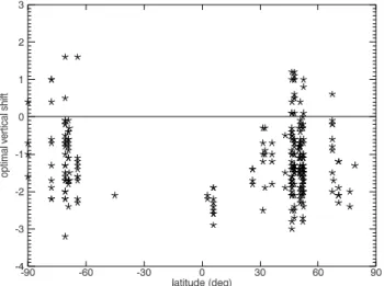
In order to find the appropriate value for this shift, we optimised the correlation between individual ozone sondes and the IFE profiles by applying different shifts, similar as was done by Segers et al. (2005). The resulting most

op-Fig. 2. Individual altitude shifts that would optimize the correlation

between IFE profiles and ozone sondes.

Table 1. Correlative data sets used in this paper. Listed are the

num-ber of stations (left) and the numnum-ber of collocations (right). Collo-cation criteria are given in Sect. 4.1.

Instrument IFE1.61 OL2.4/2.5 Lidar 6 363 6 278 Microwave 3 107 2 49

Sondes 7 30 SAGE II 884 350 SAGE III 1071

timal individual shifts are shown in Fig. 2. The spread in the shifts is much larger than the expected variation in the pointing inaccuracy. This should be expected, because dif-ferences between sondes and SCIAMACHY profiles are not only caused by pointing errors. The average shift is approx-imately −1.5 km. Therefore we chose this value for the con-stant altitude shift in this paper.

3 Correlative data sets

An overview of the correlative data sets used to study the quality of the IFE and OL data is presented in Table 1. We do not discuss the validation based on airborne campaigns conducted in 2002 and 2003 (Kuttipurath et al., 2004), be-cause no SCIAMACHY profiles were retrieved with version IFE1.61 or OL 2.4/2.5 in that timespan.

3.1 Lidar

Stratospheric ozone profiles measured by the lidars at pri-mary NDSC sites are regularly compared to measurements by other instruments, and also to a travelling lidar. This

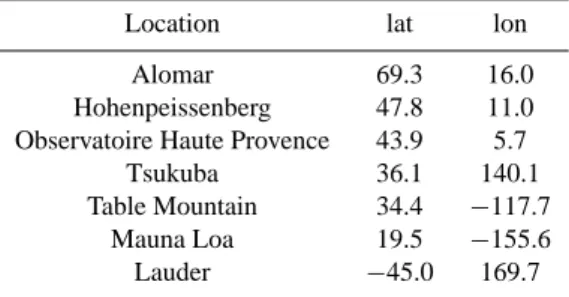
Table 2. Locations of lidar sites used in this paper.

Location lat lon Alomar 69.3 16.0 Hohenpeissenberg 47.8 11.0 Observatoire Haute Provence 43.9 5.7

Tsukuba 36.1 140.1 Table Mountain 34.4 −117.7

Mauna Loa 19.5 −155.6 Lauder −45.0 169.7

ensures their high quality measurements (e.g., McPeters et al., 1999; McDermid et al., 1998). Typical accuracies for stratospheric ozone lidar instruments are 2% for the 20 to 35 km region, and 5–10% for other altitudes (e.g., Keckhut et al., 2004). Lidar profiles are reported with a resolution of 300 m, however the correlation length is typically a few kilometers (ranging from at least 1 km in the tropopause to at most 8 km at 50 km.

Lidar measurements were taken at various midlatitude and one tropical locations, see Table 2.

3.2 Microwave instruments

3.2.1 Mauna Loa and Lauder Microwave

The instruments are groundbased microwave spectrometers observing atmospheric thermal emission at 110.8 GHz. They record the spectral lineshape of an ozone rotational transition every 20 min at about 10◦ to 20◦ elevation. Observations continue 24 h a day whenever weather permits. An ozone mixing ratio profile (in ppmv) from 56 hPa to 0.05 hPa (or 20–68 km) is retrieved for every 4–6 h period, day and night, using a semi-empirical optimal estimation retrieval method. Reference temperature and pressure profiles are used in data retrievals and in ozone mixing ratio to number density con-versions reported in the data set. Stratospheric (and meso-spheric) ozone profiles measured by microwaves at Mauna Loa and Lauder are regularly validated within the framework of NDSC. Their precision is 4–6%, accuracy 5–9% for night-time ozone profiles and daynight-time ozone profiles in the strato-sphere (Parrish et al., 1992; Connor et al., 1995). Resolution is 6–10 km below 3 hPa (about 40 km altitude) and increases to 15 km at 0.05 hPa (about 70 km altitude).

3.2.2 M´erida Microwave

The ground-based microwave radiometer MIRA 2 has been in operation on Pico Espejo near M´erida, Venezuela, since March 2004. The instrument covers the frequency range 268–281 GHz and and is capable to measure volume mixing ratio profiles of ozone, ClO, HNO3, and N2O. Ozone

verti-cal profiles in the vertiverti-cal range 20–65 km are retrieved from

measurements of the rotational transmission line at 273 GHz. The typical integration time for one profile is about 1 h and the uncertainty in the retrieved profiles due to standing waves and systematic errors amounts to at least 1 ppmv (Kopp et al., 2003). Errors due to thermal noise are almost negligible due to the integration of the measured spectra.

3.3 Sondes

Balloon based ozone sondes are launched on a regular ba-sis from globally distributed stations. A sonde samples the atmosphere up to about 30 km with a resolution of ten to hundred meters, depending on the balloon and sonde type. Ozone is measured using electro chemical cells. In a com-parison study by McPeters et al. (1999) it was shown that due to uncertainties in the composition of the chemical so-lutions, the ozone measurements from two individual sondes could show a difference of 1–2%, and that sondes agree with lidar, microwave and other measurements within 5% in the 20–45 km region.

3.4 SAGE II

The longest record of satellite high-resolution profile mea-surements has been made by the solar occultation instru-ment Stratospheric Aerosol and Gas Experiinstru-ment (SAGE II) which was launched on the Earth Radiation Budget Satellite (ERBS) in October 1984 and is still operational and collect-ing data. SAGE II uses solar occultation to measure the atten-uation of solar radiation between the satellite (McCormick, 1987). The inversion uses the “onion-peeling” approach to yield 1-km vertical resolution ozone profiles with a horizon-tal resolution of about 200 km (Mauldin et al., 1985; Chu et al., 1989). SAGE II has a repeat cycle of slightly more than a month and a vertical resolution of about 1 km. From SAGE II measurements ozone number concentrations at the 0.60 µm wavelength channel are derived (focusing on 15– 60 km). Accuracy and precision for the previous version of SAGE II (version 6.1) are characterised by Wang et al. (2002) at 16 and 53 km with an acccuracy between 5 and 7% and a precision between 3.2 and 6.7%. Validation by Wang et al. (2002) shows an agreement within 10% of SAGE II profiles with ozone sonde measurements from the tropopause up to 30 km. SAGE II v6.1 profiles slightly overestimate (less than 5%) ozone between 15 to 20 km. Extensive validation of an older version of SAGE II (version 5.96) show SAGE II to be within 7% at 20 to 50 km with correlative measurements (Cunnold et al., 1989). The version 6.2 of SAGE II was im-proved in respect to the previous version by adjustment to the aerosol clearing and by the correction of channels 520 and 1020 nm for absorption of the oxygen dimer (information on SAGE II can be found at http://www-sage2.larc.nasa.gov).

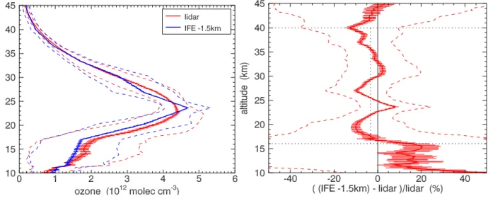
Fig. 3. Averaged profiles with their standard deviations (dashed lines) and errors (horizontal dashes) are shown in the left panel. In the right

panel, average relative differences with respect to lidar are shown as solid line, with the error on this average (defined as standard deviation of the differences divided by the square root of the number of lidar profiles (145), horizontal dashes) and the standard deviations (dashed lines). The dotted line between 16 and 40 km denotes the value of the average bias: −3% in that altitude region. An altitude shift of −1.5 km has been applied to the IFE data.

3.5 SAGE III

The Stratospheric Aerosol and Gas Experiment III (SAGE III) was launched on 10 December 2001. The instrument makes use of solar-occultation measurements, similar to those described for SAGE II above. SAGE III solar products (version 3.0) were released in mid 2004, and this is the version used in this paper. They have been intercompared with the SAGE II, HALOE, POAM III satellite instrument, and with sondes and groundbased instruments. Compared with SAGE II, a difference of 1–2% in the northern hemisphere, and about 3% in the southern hemisphere is found. These errors are independent of altitude (Taha et al., 2004).

4 SCIAMACHY IFE ozone profile validation

4.1 Validation approach

IFE ozone profile data retrieved from all available level 0 orbits during January, March, May, September, and Novem-ber 2004 were compared with groundbased lidar, microwave radiometer, and sondes. They were also compared with SAGE II and SAGE III data. Collocation criteria were a max-imum distance of 1000 km, and maxmax-imum time difference of 12 h (20 h for nighttime instruments) between SCIAMACHY overpass and correlative measurement. For SAGE III, the distance criterion was replaced by 3◦latitude and 10◦ lon-gitude. Within these limits, the nearest match between the SCIAMACHY and correlative data was selected for each

in-dividual measurement (except for comparisons with lidar, where one lidar measurement was allowed to be collocated with multiple IFE profiles, as long as the collocation criteria were met). The number of collocation profiles for the differ-ent correlative data sets are given in Table 1.

4.2 Validation results

In this subsection, we will first present comparisons in which averages were made over multiple location, and then show a few examples at unique locations.

Collocations between lidar and IFE are found only at mid-latitudes and one tropical location. Averaged over all collo-cations, we conclude that the IFE ozone profiles are lower than the lidar profiles by about 3% (16–40 km; see Fig. 3). The average difference profile has a zigzag shape with max-ima around 31 and 24 km, minmax-ima around 40, 20 and 27 km, the value varying between −10% and +10%. This shape stems from an oscillation in the IFE ozone profiles, which are likely a consequence of the fact that the air volumes sampled by SCIAMACHY at different tangent heights are not exactly aligned vertically. The maximum ozone number densities are in general too high (about 8%) compared to the lidar ozone profiles. In the lower stratosphere (18–23 km), the IFE ozone concentrations are too low.

IFE data were also compared with SAGE II data, results are shown in Fig. 4. This was done both for the original SAGE data, as well as for SAGE data that were convolved us-ing the IFE averagus-ing kernels and a prioris. SAGE II colloca-tions with IFE are mostly between 60◦S and 60◦N, with only

Fig. 4. As Fig. 3, but now with respect to SAGE II (884 collocations). For SAGE II, original profiles are shown, as well as profiles convolved

with the IFE averaging kernels using also the IFE a priori profiles.

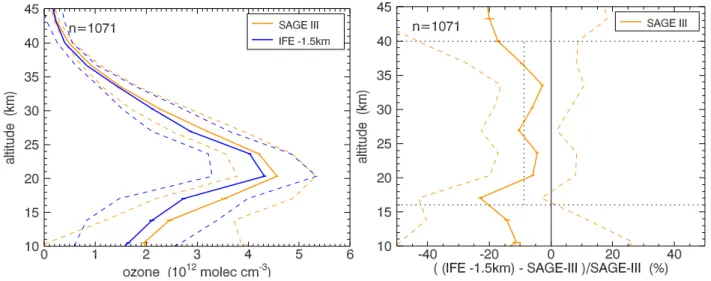
Fig. 5. As Fig. 4, but now with respect to SAGE III (1071 collocations).

a few collocations in the polar regions. Averaged over all col-locations, we see that IFE is about 6% lower than SAGE II (averaged over 16–40 km), with averaging kernels applied. Best results are found between 30 and 35 km.

As in the comparisons with lidar, we see the characteristic profile shape with IFE ozone number densities often too low around 27 km (7%). In the lower stratosphere (18–22 km), again the IFE ozone concentrations are too low, in compar-isons with SAGE II also between 16 and 18 km.

Figure 5 shows comparisons with SAGE III. This compar-ison results in a larger bias (−9% between 16 and 40 km) than the comparison with SAGE II (both with averaging ker-nels applied). Intercomparisons between the two SAGE

in-struments indicate that SAGE III is biased with respect to SAGE II: SAGE III ozone number densities are 2% higher between 15–40 km, SAGE II has a known bias below 15 km (see Sect. 3.5).

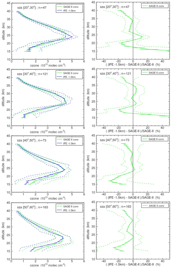
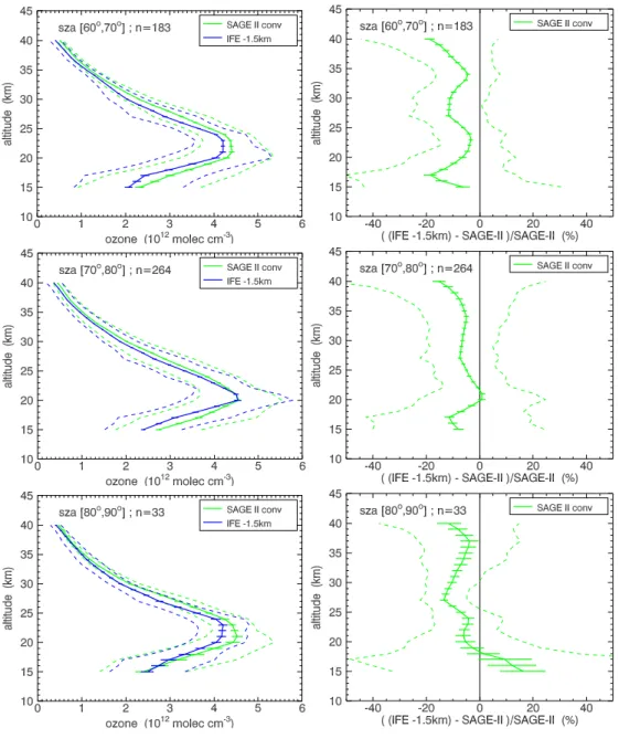
The average difference between IFE1.61 and SAGE-II profiles depends on the solar zenith angle (sza) of the SCIA-MACHY measurement. In Fig. 6, where comparisons are grouped into 10◦ sza bands, evidently the characteristic zigzag shape is present for all sza ranges, with a slight varia-tion in the altitude of the maxima and minima within 2 km.

– For sza between 50◦ and 90◦, the average IFE1.61 ozone number densities are smaller than the SAGE-II

Fig. 6. Shown here are comparisons between IFE1.61 and SAGE II, convolved with the IFE averaging kernels, grouped into 10 degree solar

Fig. 6. Continued.

values almost everywhere between 15 and 40 km. The average difference profiles are rather flat, with values ranging from −10% to 0, except for the lower levels of profiles with sza above 80◦ (+15% at 16 km) and with sza between 50◦and 60◦(−25% at 17 km).

– For sza between 20◦and 40◦the IFE1.61 profiles are on average closer to the SAGE-II profiles. The average de-viation is −1.7% between 20 and 40 km, but the peaks in the difference profile just below the ozone maximum are more pronounced, ranging from −18% at 20 km to +7% at 24 km. Below 18 km the positive difference be-comes rapidly larger.

– For sza between 40◦_{and 50}◦_{, there is no significant}

dif-ference between IFE1.61 and SAGE-II profiles between 23 and 37 km, where the zigzag shape is absent. Below 23 km the difference grows to −30% at 17 km.

We also grouped comparisons with lidar into solar zenith angle groups, namely below 30◦(56 collocations), 30◦–60◦ (235 collocations), and 60◦–90◦ (72 collocations). Solar zenith angles below 30◦ and between 30◦and 60◦give re-sults that are very similar to those shown in Fig. 3. The 60◦– 90◦sza’s show worse results, with IFE results biased low by 7% over the 15–40 km region.

When looking for a latitude dependence, we see some-thing similar, midlatitude results are biased low by about

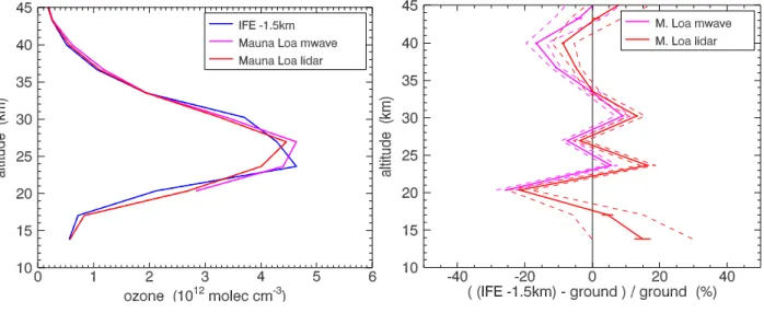
Fig. 7. As Fig. 3, but now with respect to lidar and microwave, and only for the Mauna Loa location (44 lidar-microwave-SCIAMACHY

collocations).

Fig. 8. As Fig. 3, but now with respect to microwave, only for the Merida (Venezuela) location, 15 collocations. ‘Unsmoothed data’ refer

to comparison between original IFE and microwave results, ‘smoothed data’ refer to a comparison where IFE data were smoothed using the microwave radiometer averaging kernels.

7% (15–40 km, 257 collocations), tropical results (contain-ing only Mauna Loa) are not consistently biased but do differ significantly from the lidar data (one sigma level, 106 collo-cations). In Fig. 7, we show IFE data over Mauna Loa that were collocated with lidar as well as microwave measure-mens, and therefore have fewer collocations (44). There is no significantly different result with respect to microwave than there is with respect to lidar. In Fig. 8, an example of com-parisons at another tropical location (M´erida, Venezuela) is shown. These comparisons are not consistent with those at Mauna Loa above 37 km.

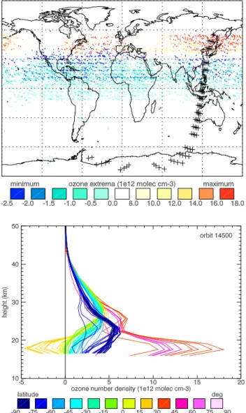
Table 3. Numbers of OL profiles with extreme values (either below

zero or above 8.0×1012cm−3).

lats total min<0.0 max>8.0

[30, 90] 2725 206 (7.5%) 972 (35%)

[−15, 30] 4938 2935 (60%) 0 (0%)

Fig. 9. Most extreme ozone concentration retrieved per profile, as

a function of location (top panel). Of the overplotted orbit (black crosses), all ozone profiles are shown in the bottom panel, where colour indicates their latitude.

There were no significantly different validation results found between each of the five months for which the IFE data were retrieved.

5 SCIAMACHY offline ozone profile verification and validation

The data set discussed here consists of OL2.4 (20 September–27 November 2004) and OL 2.5 (7 December 2004 and onward, in this paper, through 17 February 2005). Although the data are given in terms of partial columns as well as mixing ratios as a function of altitude and pressure, we will only use the partial columns, and convert these to

number densities (see the remarks in Appendix A). The col-location criteria were the same as those for the IFE data.

For the OL data, unlike the IFE data, four SCIAMACHY profiles are retrieved within one state.

5.1 Verification of SCIAMACHY offline data

Verification of the OL data shows that within the current data set, about 35% of the retrieved profiles at latitudes north of 30◦N show unrealistically high ozone concentrations be-tween about 15 and 25 km. Also, about 7.5% of the profiles north of 30◦N, and 60% of the profiles between 15◦S and 30◦N, show negative values around the tropopause region. Detailed numbers are shown in Table 3.

In Fig. 9, bottom panel, we show examples of such unre-alistic profiles for one orbit, and in the top panel we show at which locations this type of profile was found, with an indication of the most extreme (either negative or positive) value. Note that if a profile was realistic, it is not plotted. We were not able to find what caused these retrieval errors, we only verified that there was no link to ground albedo (which was assumed to be 0.3 across the globe) or to the “state IDs” (which are settings for the integration time and number of spectra taken per tangent height). Evidently, there is a clear latitude dependence (see Table 3). Also a longitudinal de-pendence was found, extreme positive values above 30◦N were found over Asia and the Atlantic (see Fig. 9), but al-most never over Europe or North America.

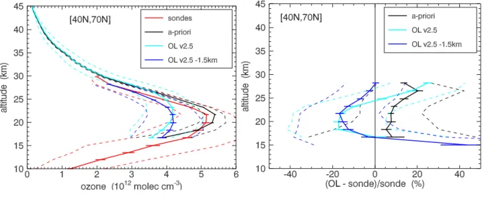
OL2.5 and the a priori profiles used in this retrieval were both compared with collocated sondes between 40 and 70◦_{N. The OL data set was first filtered to remove all profiles}

that had either ozone number densities below zero or above 8×1012cm−3_{. Also the collocated correlative data for these}

cases were filtered out. The results are shown in Fig. 10: the a prioris compare better with sondes than the retrieval. In the wavelength window where the retrieval is performed (319– 333 nm) almost no light is returned from the atmosphere be-low about 24 km (this height depends on latitude and time of year), which is evident from radiative transfer studies, e.g., see Flittner et al. (2000), that show weighting functions at 322 nm. This might explain the result.

From Fig. 10 it is not clear whether the match between sondes and retrieval above 27 km is a coincidence or a re-trieval result. The average of the unshifted rere-trievals almost perfectly match the average a priori, and the average a priori is shifted about 1.5 km with respect to the average sonde pro-file. So even if the retrieval would just return the a priori the match to the sondes would be good.

5.2 Validation of SCIAMACHY offline data

As was outlined in Sect. 2, we chose to apply a downward shift of 1.5 km to all SCIAMACHY data to correct provision-ally for the Envisat pointing inaccuracy. To assess the qual-ity of the OL2.4 and OL2.5 data above 24 km, comparisons

Fig. 10. Comparison of collocated OL2.5 (with and without a −1.5 km shift applied) and sonde ozone profiles in the Northern Hemisphere

(40–70◦N). Averaged ozone profiles and the averaged a prioris used in the OL retrieval are shown in the left panel, percent differences with respect to sondes are shown in the right panel. Dashed lines indicate one standard deviation divided by the square root of the number (30) of collocations. Evidently, the OL2.5 data compare worse than their own a prioris for altitudes of 24 km and lower.

with groundbased lidar and microwave were made, as well as with SAGE II. Averaging kernels were not available. Outliers like those discussed in the previous subsection were removed from the averages. Results below 24 km confirm that the ozone maximum is underestimated (by up to 20% at 20 km). In Fig. 11 we show comparisons of OL2.4 and OL2.5 (to-gether) with lidar. The number of collocations was 86 and 192, respectively. We see that OL profiles above 24 km agree with lidar results to within 2σ . They disagree significantly between 20 and 24 km (15±5% too low).

These results are consistent with comparisons performed with SAGE II and microwave (not shown). A similar latitude dependence that was described for the IFE data (Sect. 4.2) was evident from the OL (2.4. and 2.5 together) to SAGE II comparisons: at the NH mid latitudes, SCIA OL profiles seem to deviate more than in the other regions. Retrievals in the SH do not show this latitude dependence.

The retrieval above 40 km and below 15 km will stay close to the a priori. It is therefore expected that the altitude shift applied to the retrieved profile causes the ozone values to be smaller than the a priori above 40 km, and larger than the a priori below 15 km. When we assume that the a priori is close to the true profile for these heights, we would expect the altitude shifted SCIAMACHY profile to have smaller values than the true profile above 40 km, and larger values than the true profile below 15 km. This is indeed what can be seen in Figs. 10 and 11.

6 Conclusions and outlook

We validated the SCIAMACHY ozone profiles retrieved us-ing the IFE algorithm version 1.61 with various correlative instruments. The standard deviation of the differences is typ-ically 10% between 20 and 35 km. The IFE profiles are bi-ased low by 3 to 6% with respect to lidar and SAGE II, re-spectively. There is a solar zenith angle dependence in these results, which is discussed in detail. For solar zenith angles below 30◦(typically in the tropics) the average bias between 20 and 40 km is −1.7% compared to SAGE II.

The IFE algorithm is under development. A future version will probably include a radiative-transfer based correction for the inaccurate Envisat pointing, which was described in an earlier paper (Kaiser et al., 2004)

More than 20% of the OL ozone profiles version 2.4 and 2.5 have unrealistic ozone values, most of these are north of 15◦S. The remaining OL profiles compare well to lidar and SAGE II above 24 km. Between 20 and 24 km, they under-estimate ozone by 15±5%. There are indications that the retrieval is very restrained to the a priori. A new offline al-gorithm is currently under development (DLR, private com-munication, 2005). In this new OL algorithm, a different fit window, similar to that now used in the IFE algorithm, will be applied.

Fig. 11. As Fig. 3, but here OL data versions 2.4 and 2.5 (together) are compared with 42 collocated lidar profiles.

Appendix A

Remarks on SCIAMACHY offline data set

Since documentation of the offline data is currently not avail-able, we will make a few remarks for the benefit of potential users of these data.

– Profiles are reported in terms of partial columns and

in mixing ratio. Mixing ratio profiles were generated from the partial columns using a very crude tempera-ture and pressure climatology, and are therefore subject to large errors. Users who need mixing ratio units can get more accurate results by converting the reported par-tial columns into number density, and then into mixing ratio using appropriate (e.g., NCEP or ECMWF) tem-perature and pressure profiles.

– The temperature and pressure profiles reported in the

files are climatological values and were not retrieved.

– The averaging kernels of the profiles are not reported.

This means that true validation cannot be carried out. The a prioris can be deduced by applying the reported iterative change to the profile in each of the retrieval steps backwards.

Acknowledgements. This research was funded in part by the

Netherlands Agency for Aerospace Programmes (NIVR), by ESA under the SciLoV project, and by BMBF under the project DLR 50EE0502. Lidar measurements used in this work were partly funded by ESA under the EQUAL validation projects. We acknowledge the use of ozone profile observations from the Envisat-NILU, the WOUDC, and the NDSC databases. We acknowledge the help of DLR personnel for useful discussions about the offline data retrieval.

Edited by: P. C. Simon

References

Bracher, A., Bovensmann H., Bramstedt K., Burrows J. P., von Clar-mann T., et al.: Cross comparisons of O₃and NO₂profiles mea-sured by the atmospheric Envisat instruments GOMOS, MIPAS, and SCIAMACHY, Adv. Space Res., in press, 2005.

Bovensmann, H., Burrows, J. P., Buchwitz, M., Frerick, J., No¨el, S., Rozanov, V. V., Chance, K. V., and Goede, A. P. H.: SCIA-MACHY: Mission objectives and measurement modes, J. Atmos. Sci., 56, 2, 127–150, 1999.

Brinksma, E. J., Piters, A. J. M., Boyd, I. S., Parrish, A., Bracher, A., et al.: Sciamachy Ozone Profile Validation, Proceedings of the Second Workshop on the Atmospheric Chemistry Valida-tion of Envisat (ACVE-2), 3–7 May 2004, ESA-ESRIN, Frascati, Italy (ESA SP-562), 2004.

Chu, W. P., McCormick, M. P., Lenoble, J., Brogniez, C., and Pru-vost, P.: SAGE II inversion algorithm, J. Geophys. Res., 94, 8339–8351, 1989.

Connor, B. J., Parrish, A., Tsou, J.-J., and McCormick, P.: Er-ror analysis for the ground-based microwave ozone measurement during STOIC, J. Geophys. Res., 100(D5), 9283–9291, 1995. Cunnold, D. M., Chu, W. P., Barnes, R. A., McCormick, M. P., and

Veiga, R. E.: Validation of SAGE II Ozone Measurements, J. Geophys. Res., 94, 8447–8460, 1989.

De Clercq, C., Lambert, J.-C., Calisesi, Y., Claude, H., Stubi, R., von Savigny, C., and the ACVT-GBMCD Ozone Profile Team: Integrated characterization of Envisat ozone profile data using ground-based network data, Proceedings of the Envisat & ERS Symposium, Salzburg, Austria, 6–10 September 2004, ESA SP-572, 2004.

Flittner, D. E., Bhartia, P. K., and Hermann, B. M.: O3profiles

re-trieved from limb scatter measurements: Theory, Geophys. Res. Lett., 27(17), 2601–2604, 2000.

Kaiser, J.: Retrieval from Limb Measurements, PhD Thesis, Uni-versity of Bremen, Germany, 2001.

Kopp, G., Berg, H., Blumenstock, Th., Fischer, H., Hase, F., Hochschild, G., H¨opfner, M., Kouker, W., Reddmann, Th.,

Ruhnke, R., Raffalski, U., and Kondo, Y.: Evolution of ozone and ozone related species over Kiruna during the THESEO 2000-SOLVE campaign retrieved from ground-based millimeter wave and infrared observations, J. Geophys. Res., 108(D5), 8308, doi:10.1029/2001JD001064, 2003.

Kaiser, J., Von Savigny, C., Eichmann, K.-U., No¨el, S., Bovens-mann, H., and Burrows, J.: Satellite-pointing retrieval from at-mospheric limb-scattering of solar UV-B radiation, Can. J. Phys., 82, 1041–1052, doi:10.1193/P04-071, 2004.

Keckhut, P., McDermid, S., Swart, D., McGee, T., Godin-Beekmann, S., et al.: Review of ozone and temperature lidar val-idations performed within the framework of the Network for the Detection of Stratospheric Change, J. Environ. Monit., 6, 721– 733, 2004.

Kuttippurath, J., Kleinb¨ohl, A., Bremer, H., K¨ullmann, H., and Notholt, J.: Validation of SCIAMACHY ozone limb profiles by ASUR, Proceedings of the Second Workshop on the Atmo-spheric Chemistry Validation of Envisat (ACVE-2), 3–7 May 2004, ESA-ESRIN, Frascati, Italy (ESA SP-562).

Mauldin III, L. E., Zuan, N. H., McCormick, M. P., Guy, J. H., and Vaughn, W. R.: Stratospheric Aerosol and Gas Experiment: A functional description, Opt. Eng., 24, 307–312, 1985.

McCormick, M. P.: SAGE II: An overview, Adv. Space Res., 7(3), 219–226, 1987.

McDermid, I. S., Bergwerff, J. B., Bodeker, G., Boyd, I. S., Brinksma, E. J., et al.: OPAL: Network for the Detection of Stratospheric Change Ozone Profiler Assessment at Lauder, New Zealand. II. Intercomparison of Revised Results, J. Geophys. Res., 103, 28 693–28 699, 1998.

McPeters, R. D.: Ozone profile comparisons, in: The atmospheric effects of stratospheric aircraft, Report of the 1992 models and measurements workshop, NASA reference publication 1292, edited by: Prather, M. J. and Remsberg, E. E., D31–D37, 1993. McPeters, R. D., Hofmann, D. J., Clark, M., Flynn, L., Froidevaux,

L., et al.: Results from the 1995 Stratospheric Ozone Profile Intercomparison at Mauna Loa, J. Geophys. Res., 104, 30 505– 30 514, 1999.

Palm, M., von Savigny, C., Warneke, T., Velazco, V., Notholt, J., K¨unzi, K., Burrows, J., and Schrems, O.: Intercomparison of O₃profiles observed by SCIAMACHY, ground based microwave and FTIR instruments, Atmos. Chem. Phys. Discuss., 5, 911– 936, 2005,

SRef-ID: 1680-7375/acpd/2005-5-911.

Parrish, A., Connor, B. J., Tsou, J. J, McDermid, I. S., and Chu, W. P.: Ground-based Microwave Monitoring of Stratospheric Ozone, J. Geophys. Res., 97(D2), 2541–2546, 1992.

Segers, A. J., von Savigny, C., Brinksma, E. J., and Piters, A. J. M.: Validation of IFE-1.6 SCIAMACHY limb ozone profiles, Atmos. Chem. Phys., 5, 3045–3052, 2005,

SRef-ID: 1680-7324/acp/2005-5-3045.

von Savigny, C., Rozanov, A., Bovensmann, H., Eichmann, K.-U., No¨el, S., Rozanov, V. V., Sinnhuber, B.-M., Weber, M., and Bur-rows, J.: The ozone hole breakup in September 2002 as seen by SCIAMACHY on Envisat, J. Atmos. Sci., 62(3), 721–734, 2005a.

von Savigny, C., Kaiser, J. W., Bovensmann, H., McDermid, I. S., Leblanc, T., and Burrows, J.: Spatial and Temporal Characteri-zation of SCIAMACHY Limb Pointing Errors During the First Three Years of the Mission, Atmos. Chem. Phys., 5, 2593–2602, 2005b,

SRef-ID: 1680-7324/acp/2005-5-2593.

Taha, G., Thomason, L. W., Trepte, C., and Chu, W. P.: Valida-tion of SAGE III Data Products Version 3.0, Quadrennial Ozone Symposium, QOS, 1–8 September, 2004, Kos, Greece, Proceed-ings of QOS, pp. 115–116, 2004.

Wang, H.-J., Cunnold, D. M., Thomason, L. W., Zawodny, J. M., and Bodeker, G. E.: Assessment of SAGE II version 6.1 ozone data quality, J. Geophys. Res., 107(D23), 4691, doi:10.1029/2002JD002418, 2002.