HAL Id: insu-03171037
https://hal-insu.archives-ouvertes.fr/insu-03171037
Submitted on 17 Mar 2021
HAL is a multi-disciplinary open access
archive for the deposit and dissemination of
sci-entific research documents, whether they are
pub-lished or not. The documents may come from
teaching and research institutions in France or
abroad, or from public or private research centers.
L’archive ouverte pluridisciplinaire HAL, est
destinée au dépôt et à la diffusion de documents
scientifiques de niveau recherche, publiés ou non,
émanant des établissements d’enseignement et de
recherche français ou étrangers, des laboratoires
publics ou privés.
Distributed under a Creative Commons Attribution| 4.0 International License
Variations of the peak positions in the longitudinal
profile of noon-time equatorial electrojet
Zié Tuo, Vafi Doumbia, Pierdavide Coïsson, N’guessan Kouassi, Abdel Aziz
Kassamba
To cite this version:
Zié Tuo, Vafi Doumbia, Pierdavide Coïsson, N’guessan Kouassi, Abdel Aziz Kassamba. Variations
of the peak positions in the longitudinal profile of noon-time equatorial electrojet. Earth Planets
and Space, Springer/Terra Scientific Publishing Company, 2020, 72 (1), �10.1186/s40623-020-01305-z�.
�insu-03171037�
FULL PAPER
Variations of the peak positions
in the longitudinal profile of noon-time
equatorial electrojet
Zié Tuo
1*, Vafi Doumbia
1, Pierdavide Coïsson
2, N’Guessan Kouassi
1and Abdel Aziz Kassamba
1Abstract
In this study, the seasonal variations of the EEJ longitudinal profiles were examined based on the full CHAMP satel-lite magnetic measurements from 2001 to 2010. A total of 7537 satelsatel-lite noon-time passes across the magnetic dip-equator were analyzed. On the average, the EEJ exhibits the wave-four longitudinal pattern with four maxima located, respectively, around 170° W, 80° W, 10° W and 100° E longitudes. However, a detailed analysis of the monthly averages yielded the classification of the longitudinal profiles in two types. Profiles with three main maxima located, respectively, around 150° W, 0° and 120° E, were observed in December solstice (D) of the Lloyd seasons. In addition, a secondary maximum observed near 90° W in November, December and January, reinforces from March to October to establish the wave-four patterns of the EEJ longitudinal variation. These wave-four patterns were divided into two groups: a group of transition which includes equinox months March, April and October and May in the June solstice; and another group of well-established wave-four pattern which covers June, July, August of the June solstice and the month of September in September equinox. For the first time, the motions in the course of seasons of various maxima of the EEJ noon-time longitudinal profiles have been clearly highlighted.
Keywords: Equatorial electrojet, Longitudinal variation, Seasonal dependence
© The Author(s) 2020. This article is licensed under a Creative Commons Attribution 4.0 International License, which permits use, sharing, adaptation, distribution and reproduction in any medium or format, as long as you give appropriate credit to the original author(s) and the source, provide a link to the Creative Commons licence, and indicate if changes were made. The images or other third party material in this article are included in the article’s Creative Commons licence, unless indicated otherwise in a credit line to the material. If material is not included in the article’s Creative Commons licence and your intended use is not permitted by statutory regulation or exceeds the permitted use, you will need to obtain permission directly from the copyright holder. To view a copy of this licence, visit http://creat iveco mmons .org/licen ses/by/4.0/.
Introduction
The equatorial electrojet (EEJ) is a daytime ionospheric current that flows eastward along the magnetic equator at about 105 km altitude (Chapman 1951). Most of the EEJ characteristics like day-to-day, seasonal, latitudi-nal, longitudinal variability and the counter-electrojet phenomenon have been described through its magnetic effect recorded on ground as well as onboard polar orbit-ing satellites (Cain and Sweeney 1973; Gouin 1967; Guru-baran 2002; Langel et al. 1993). During the International Equatorial Electrojet Year (IEEY), simultaneous meas-urements were carried out in the longitude sectors of Asia, Africa and South America (Amory-Mazaudier et al.
1993; Arora et al. 1993). Magnetic data recorded along
station chains across the dip-equator resulted in impor-tant advances for understanding the EEJ characteristics. Based on this dataset, Doumouya et al. (2003) estab-lished the longitudinal profile of EEJ, which was found to be inversely correlated with the geomagnetic main field intensity. However, Doumouya and Cohen (2004) noticed a relative amplified EEJ intensity in the longitude sector around 100° E when they included the magnetic data from Baclieu (105.44° E, 9.25 N 1.35° dip-lat) in Viet-nam. This observation was confirmed by the CHAlleng-ing Minisatellite Payload (CHAMP) satellite magnetic data (Doumouya and Cohen 2004). The geomagnetic field measurements operated onboard Satelite de Appli-caciones Cientificas-C (SAC-C), Oersted and CHAMP satellites resulted in improved descriptions of the EEJ longitudinal variation (Alken and Maus 2007; Doumouya and Cohen 2004; Jadhav et al. 2002). Thus, the EEJ lon-gitudinal profiles are now known to exhibit up to three or four maxima located approximately around − 90° E, 0°,
Open Access
*Correspondence: [email protected]
1 Laboratoire de Physique de l’Atmosphère et de Mécanique des fluides, UFR-SSMT, Université Felix Houphouet Boigny, Abidjan, Côte d’Ivoire Full list of author information is available at the end of the article
Page 2 of 9 Tuo et al. Earth, Planets and Space (2020) 72:174
100° E and 180° E (Alken and Maus 2007; Doumbia et al.
2007; Doumbia and Grodji 2016; Doumouya and Cohen
2004; Jadhav et al. 2002). According to Alken and Maus (2007), Doumbia et al (2007) and Doumbia and Grodji (2016), these longitudinal structures of the EEJ can be subject of seasonal variations. Indeed, it was shown that the EEJ longitude profiles with three maxima are observed during the December solstice, while the profiles with four maxima are observed during equinoxes and the June solstice. However, the transitions between the EEJ longitudinal patterns of three maxima and those of four maxima and the background physical processes are not well understood.
In the present study, the seasonal variations of the EEJ longitudinal structures are examined. In that purpose the longitudinal variation of the EEJ is revisited from the full CHAMP satellite magnetic data recorded from 2001 to 2010. In particular, the progressive changes from three maxima to four maxima, and vice versa, of the EEJ lon-gitude patterns in the course of the year is analyzed on the basis of the average monthly longitude profiles. The motions of the upper mentioned maxima according to the seasons are also examined.
Data and data processing
Data
The present work is based on CHAMP satellite OVer-hauser Magnetometer (OVM) data that were recorded from 2001 to 2010 (Rother and Michaelis 2019) (https ://isdc-old.gfz-potsd am.de/index .php). CHAMP was a near-polar orbiting satellite that was launched on July 15, 2000 onto a low altitude (about 460 km) circular orbit, with an inclination of 87.3° and orbital period of 93.55 min (Alken and Maus 2007; Lühr et al. 2004; Lühr and Maus 2006). The satellite was deorbited on Septem-ber 19, 2010. One of the advantages of CHAMP orbit is that it provides a good latitudinal and local time cover-age allowing accurate studies of the ionospheric current systems.
The geomagnetic force F was recorded with the OVM magnetometer at a sampling rate of 1 s, in the range from 18,000 to 65,000 nT, with 10 pT resolution and noise level of 50 pT. The absolute error is estimated at about 0.5 nT. The magnetic data recorded on board CHAMP satellites are composed of the sum of the geomagnetic main field, the crustal anomaly fields, the magnetic effects of iono-spheric and magnetoiono-spheric currents and their induced effects in the ground. Thus, any study of one of these sources requires its contribution to be isolated from that of the other magnetic sources. The purpose of the present work is to study the EEJ by analyzing its magnetic effect, extracted from the total observed magnetic force F.
Data processing
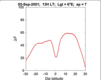
The geomagnetic main field that represents about 99% of the total measured field, is estimated and removed by using the International Geomagnetic Reference Field (IGRF-12) model (Thébault et al. 2015). The remaining residual field, shown in Fig. 1, is designated as total resid-uals (�F) . ( F ) is expected to include the crustal fields and the magnetic effects of ionospheric and magneto-spheric currents. The EEJ magnetic effect is confined to a relative narrow latitude band and produces a V-shape depression at the magnetic dip-equator. This effect seems to overlap a long-wavelength background signal, from which it will be isolated. The approach consists of poly-nomial fitting of the background signal (Doumouya and Cohen 2004).
For this study, magnetically quiet time data are selected according to the values of the Kp index that is set to be
smaller than 3+. Noon-time data for satellite passes
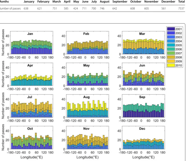
between 11 and 13 LT are considered to estimate the EEJ strength ( Feej ). Table 1 depicts the numbers of satellite
noon-time passes selected per month. Figure 2 shows the monthly distribution of satellite passes per year. A total number of 7537 noon-time satellite passes have been selected.
Extracting the EEJ magnetic effect by using a polynomial fitting
The magnetic effect of the EEJ was extracted from the total magnetic residuals by subtracting the background signal (Fig. 3). The background signal was fitted with a 12-degree polynomial. This degree was chosen by trial-and-error testing from 6° to 30° (Doumbia and Grodji
Fig. 1 The total residuals ( F) isolated from the CHAMP satellite
observed total force ( F ) by subtracting the geomagnetic main field estimated with IGRF model
2016; Doumouya and Cohen 2004). The solid line repre-sents the total residuals and the dashed line reprerepre-sents the polynomial fitting of the background signal. The right panel of Fig. 3 shows the latitudinal profiles of the EEJ magnetic effect extracted for a CHAMP satellite pass across the dip-equator at 1° E on 17 September 2001. The EEJ magnetic effect exhibits a sharp depression with a minimum at the dip-equator. This depression is flanked by two maxima that are located on the average at about ± 7◦ on either side of the magnetic dip-equator. The dif-ference in amplitudes for the same day may be due to the longitudinal dependence of the EEJ. For different days,
this difference also includes the day-to-day variability of the EEJ. (Doumouya and Cohen 2004; Thomas et al.
2017).
Correction of satellite altitude effects on the EEJ strength
The CHAMP satellite mission lasted about 10 years from 2000 to 2010. This duration is close to the length of one solar cycle. During this period, the satellite orbit continu-ously drifted from the initial altitude of 460 km to 250 km at the end of the mission (Fig. 4). The decreasing altitude of CHAMP gradually moved it closer to the EEJ. As a consequence, the observed EEJ effects may have gradually
Table 1. Monthly distribution of selected noon-time satellite passages between 11 LT and 13 LT during geomagnetically quiet days with Kp < 3+.
Months January February March April May June July August September October November December Total
Number of passes 638 621 751 585 424 711 700 746 642 608 605 561 7537
Page 4 of 9 Tuo et al. Earth, Planets and Space (2020) 72:174
increased due to the decreasing distance between the sat-ellite and the EEJ current, located at about 105 km alti-tude. Thus, variations of the observed EEJ strength can be expected to include both the effects of the solar cycle and the satellite altitude variations. In this section, we reduce the effects of satellite altitude variations. The altitude effect correction consists of normalizing the measure-ments to 400 km altitude applying Eq. (1). This method is based on Le Mouël et al. (2006) appendix.
where F400 is the EEJ strength at h400= 400 km, Fsat
is the EEJ strength at a given altitude hsat , hsat is the
dis-tance between the satellite and the EEJ altitude. h400 is
the distance between the normalized altitude and the EEJ altitude. (1) F400= hsat h400 Fsat,
Fig. 3 The magnetic signature of the equatorial electrojet (EEJ). The left panel shows the total residuals F (solid line) and background long wave
length signal (dashed line). The right panel shows the EEJ magnetic signature isolated from the total residuals
Results
Longitudinal variation of EEJ
The EEJ strength ( Feej ) is estimated from the
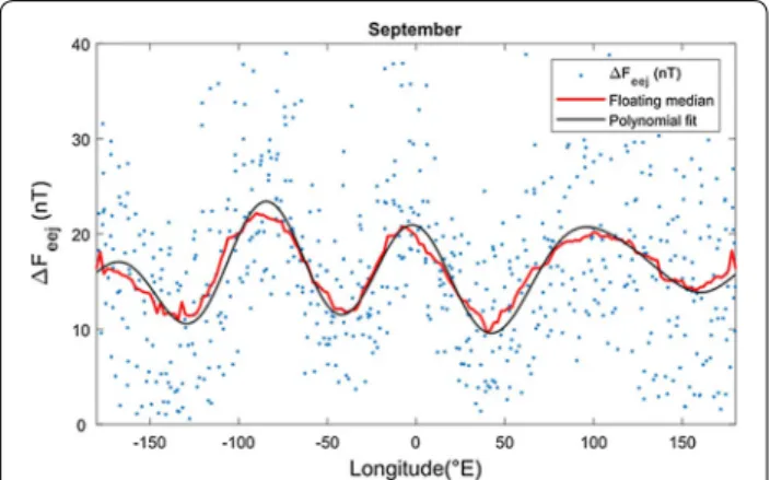
latitudi-nal profiles by the difference between the minimum at the dip-equator and the average of the maxima on either side for each satellite pass across the magnetic equa-tor. Figure 5 depicts the average longitudinal variation of the EEJ during September equinox. The dots repre-sent Feej for single satellite passes across the
dip-equa-tor. The solid red line shows the median values of Feej
over every 15-degree longitude interval from − 180° E to 180° E and the smoothed black line is obtained by spline interpolation of the median values. The four maxima located, respectively, at about − 170° E, − 80° E, − 10° E and 100° E longitudes confirm the four-wave structure of the EEJ longitudinal variation, shown in previous studies (Alken and Maus 2007; Doumbia et al. 2007; Le Mouël et al. 2006; Yamazaki and Maute 2017). This structure is susceptible to seasonal variations that are examined in the next section.
Seasonal variation of EEJ longitudinal profiles
Figure 6 shows the monthly averages of the EEJ longi-tudinal variations. The blue and green curves repre-sent, respectively, the first quartile (25% of data) and third quartile (75% of data). The solid red line and the smoothed black line are the same as Fig. 5. The pat-terns of the EEJ longitudinal profiles evolve from month to month. These patterns can be divided into two main kinds. Profiles with three maxima are observed from November to February, while those with four maxima, referred to as “wave-four” pattern are observed from March to October. The patterns with three maxima are mainly observed during the December solstice, while
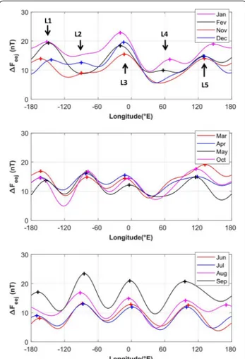
the wave-four patterns include June solstice, March and September equinoxes. However, the patterns observed from March to May and in October seem to be transi-tion phases between the three maxima and wave-four patterns. According to these remarks, the longitudinal profiles of the EEJ are classified into three categories in Fig. 7. In the top panel, the EEJ longitudinal profiles with three maxima are shown. These profiles exhibit three main maxima that are located, respectively, from left to right, near − 150° E, 0° E and 120° E, which are referred to as L1, L3 and L5. However, on the west side, one can observe a secondary maximum near − 90° E (L2) in November and December, which is slightly vis-ible in January, but totally vanished in February. On the east side, another secondary maximum can be observed near 70° E (L4) in January and February. In the middle panel, in addition to the three main maxima observed above, the west side secondary maximum (L2) stabilizes and gets matured at about − 80° E, while the east side secondary maximum (L4) is slightly visible in March and April, but totally vanished in May and it does not appear in October. It is as if this secondary maximum (L4) and the east side main maximum (L5) combine to form a sin-gle maximum around 120° E. This process completes the wave-four pattern establishment as depicted in the bot-tom panel. In summary, we have two west side maxima around about − 150° E, − 80° E, one maximum around 0° E and another maximum around 100° E.
Figure 8 shows the motions of the maxima in lon-gitude in the course over a year. It is to be noticed that the locations L1, L3 and L5 of the three main maxima move, respectively, over 50°, 20° and 60° longitudes in the course of the year. They oscillate, respectively, around the meridians − 160° E, − 10° E and 120° E. L1 and L5 move in the same phase from the east sides to the west side of the − 160° E and 120° E meridians, respectively, while L3 moves from the west side to the east side of the − 10° E meridian, in opposite phase with respect to L1 and L5. However, during the transition phase, while L1 seems to stabilize at − 160° E, L5 moves across the 120° E meridian westward from March to May and eastward in October. L2 is almost stable at − 80° E meridian in the transition phase and moving very little to east during the rest of time. L4 appears on January at 70° E and move to 55° E on February before combining with L5 during March and April.
Discussion and conclusion
In this study, the seasonal variations of the EEJ longi-tudinal profiles were examined based on CHAMP sat-ellite magnetic measurements from 2001 to 2010. 7537 satellite noon-time passes across the magnetic dip-equator were analyzed. The EEJ strength was estimated
Fig. 5 Longitudinal variation of the EEJ during September equinox.
The dots represent the EEJ strength estimated from single noon-time passes, the solid lines represent linear interpolation (red line) and spline interpolation (black line) of the median values of the EEJ strength in every 15° longitude
Page 6 of 9 Tuo et al. Earth, Planets and Space (2020) 72:174
from the latitudinal profiles of its magnetic signatures, with dense coverage of all longitude sectors. Based on these results, the EEJ longitudinal variation was revis-ited. On the average, the EEJ exhibits the wave-four longitudinal pattern with four maxima located, respec-tively, around − 170° E, − 80° E, − 10° E and 100° E lon-gitudes. This confirms the results obtained in previous studies (Alken and Maus 2007; Doumbia et al. 2007; Doumbia and Grodji 2016; Doumouya and Cohen 2004; Jadhav et al. 2002; Lühr et al. 2004). However, a detailed analysis of the monthly averages yielded the classifica-tion of the longitudinal profiles in two types. Profiles with three main maxima located, respectively, around − 150° E, 0° E and 120° E, were observed in Novem-ber, DecemNovem-ber, January and February. In addition, a secondary maximum observed near − 90° E started in
November, December and slightly in January, to finally establish the wave-four patterns from March to Octo-ber. It is to be noticed that the period of wave-four pat-terns includes the months of equinoxes (E) and June solstice (J) of Lloyd seasons. According to our observa-tions, this period was divided into a period of transi-tion (March, April, May and October) and a period of well-established wave-four structure (June, July, August and September). The period of transition includes two phases. The first phase consists of transition from three to four maxima in March, April and May, and the sec-ond phase consists of a short transition from four to three maxima during October. In summary, the pat-terns the EEJ longitudinal variation have been divided into three groups of 4 months each: (i) the group of three maxima, (ii) the group of transition and (iii) the
Fig. 6 Monthly average noon-time longitudinal variations of the EEJ. The dots represent the EEJ strength estimated from single noon-time passes,
the solid lines represent linear interpolation (red line) and spline interpolation (black line) of the median values of the EEJ strength in every 15° longitude. The blue and green lines represent, respectively, the spline interpolations of the first and third quartile values of the EEJ strength in every 15° longitude
group of well-established wave-four pattern. While the first group coincides with December solstice (D) of the Lloyd seasons, the second group spans partially on the equinox (March, April and October) and June solstice (May), the third group covers partially June solstice (June, July and August) and equinox (September).
The locations of the three main maxima of the EEJ lon-gitudinal profiles identified from West to East, respec-tively, as L1, L3 and L5, have been found to clearly oscillate around average positions in longitude. Thus, L1 and L5 move from the east sides to the west side of, respectively, − 160° E and 120° E meridians, while L3 moves from the west side to the east side of − 10° E meridian. During the transition phase, L1 stabilizes at − 160° E and L5 moves westward across 120° E meridian
from March to May and eastward in October. In the tran-sition phase, L2 almost stabilizes at − 80° E meridian, moving very little to east during the rest of time. Another secondary maximum (L4) was also observed near 70° E, but only in January and February.
The results above clearly demonstrate the dependence of the EEJ longitudinal structures on season and confirm the finding of previous studies by Alken and Maus (2007), Doumbia et al (2007) and Doumbia and Grodji (2016). Indeed, those studies have shown that the EEJ longitudi-nal profiles with three maxima were observed during the December solstice, while the profiles with four maxima were observed during equinoxes and the June solstice of Lloyd seasons. However, results are slightly different for the transition phases and well-established wave-four structures, which are instead inter-seasonal. In addition, it is the first time that the motions of various maxima of the EEJ longitudinal structures have been clearly high-lighted. The original features of the present work can be summarized as:
1. The full CHAMP satellite 10-year magnetic data base was used, which statistically better supports the kind of detailed analysis conducted in this manuscript. 2. Previous works (Alken and Maus 2007; Doumbia
et al. 2007; Doumbia and Grodji 2016; Doumouya and Cohen 2004; Jadhav et al. 2002; Lühr et al. 2004) have only made broad remarks on the EEJ longitudi-nal variations and attributed different morphologies to December solstice (three maxima) and four max-ima for the other seasons. In the present study, these features of the EEJ longitude profiles are captured more finely on a monthly basis.
Fig. 7 Different configurations of the EEJ longitudinal structures. In
the top panel, the EEJ longitudinal profiles with three main maxima corresponding to December solstice are shown. The middle panel shows the wave-four patterns the EEJ longitude profiles in the transition phases during March, April, May and October. The bottom panel exhibits well-established wave-four patterns from June to September. L1, L2, L3, L4 and L5 and plus symbol indicate the locations of various maxima
Fig. 8 Motions of the maxima in longitude in the course of a year.
The color zones depict the three categories of EEJ longitudinal profiles shown in the figure. The yellow zone corresponds to the periods of dominant three maxima (NDJF), the blue to the periods of transition (MAMO) and the pink to the periods of dominant wave-four patterns (JJAS)
Page 8 of 9 Tuo et al. Earth, Planets and Space (2020) 72:174
3. The present study yielded for the first time a special classification of the EEJ longitude profiles in three main categories as shown in this manuscript. In
addition, we have shown how transitions are made from one structure to the other.
4. Our classification shows that most of the features of the EEJ longitude profiles are inter-seasonal, instead of coinciding with a single particular season.
5. The motions in longitudes of different maxima of the EEJ longitude profiles in course of the year were examined the first time.
6. These new features open the way to better perspec-tives in the analysis of the physical processes that govern the EEJ longitudinal variation, especially the roles of thermospheric winds and their seasonal behaviors in this longitudinal variation (England et al.
2006; Immel et al. 2006; Lühr et al. 2008).
The structures and seasonal dependence of the EEJ longitudinal variation have been considered to be linked with the wave structures of the thermospheric winds (Doumbia et al. 2007; Doumbia and Grodji 2016; Immel et al. 2006; Kil et al. 2007; Lühr et al. 2008; Lühr and Maus 2006). In the ionosphere, winds and electric fields are known to be modulated by the tidal excitations that propagate upward from lower atmospheric layers. Doumbia et al. (2007) simulated such tidal excitations for migrating tides diurnal and semi-diurnal components based on the National Center for Atmospheric Research Thermosphere–Ionosphere Electrodynamics General Circulation Model (NCAR TIEGCM). Furthermore, the wave structures of the thermospheric winds described in many studies (Häusler et al. 2007; Häusler and Lühr 2009; Immel et al. 2006), have been found to exhibit similar longitudinal variations. In a companion paper, the influ-ence of thermospheric winds will be examined with com-bined migrating and non-migrating tidal excitations, for a better understanding of the background physical pro-cesses involved in the transition between the various EEJ longitudinal patterns.
Abbreviations
EEJ: Equatorial electrojet; IEEY: International Equatorial Electrojet Year; OVM: OVerhauser Magnetometer; CHAMP: CHAllenging Minisatellite Payload; SAC-C: Satelite de Aplicaciones Cientificas-C.
Acknowledgements
We are grateful to the German Aerospace Center (DLR) and (GFZ) for making CHAMP data available for this study. This work was partially carried out at the Institut de physique du globe de Paris (IPGP) during a visit of Mr Tuo Zié that was financially supported by PASRES (Programme d’Appui Stratégique à la Recherche Scientifique).
Authors’ contributions
The present work was performed in the framework of the Ph.D. thesis of Zié Tuo, under the supervision of Professor Vafi Doumbia in collaboration with Dr.
Pierdavide Coïsson. Zié Tuo, Vafi Doumbia and Pierdavide Coïsson contributed to the data processing and analysis. Vafi Doumbia and Pierdavide Coïsson veri-fied the analytical methods and the findings of the manuscript and contrib-uted to the discussions of the results. All the authors contribcontrib-uted to the final manuscript submitted. All authors read and approved the final manuscript.
Funding
PASRES (Programme d’Appui Stratégique à la Recherche Scientifique) sup-ported 5 months stay at the Institut de physique du globe de Paris (IPGP) in Paris for part of this work.
Availability of data and materials
The CHAMP satellite magnetic data and the Kp were available on Geo-ForschungsZentrum (GFZ) database (https ://isdc-old.gfz-potsd am.de/index .php).
Competing interests
The authors declare that they have no competing interests.
Author details
1 Laboratoire de Physique de l’Atmosphère et de Mécanique des fluides, UFR-SSMT, Université Felix Houphouet Boigny, Abidjan, Côte d’Ivoire. 2 Univer-sité de Paris, Institut de Physique du Globe de Paris, CNRS, 75005 Paris, France. Received: 24 June 2020 Accepted: 30 October 2020
References
Alken P, Maus S (2007) Spatio-temporal characterization of the equatorial electrojet from CHAMP, Ørsted, and SAC-C satellite magnetic measure-ments: empirical model of the EEJ. J Geophys Res Space Phys. https ://doi. org/10.1029/2007J A0125 24
Amory-Mazaudier C, Vila P, Achache J, Achy-Seka A, Albouy Y, Blanc E, Boka K, Bouvet J, Cohen Y, Dukhan M, Doumouya V, Fambitakoye O, Gendrin R, Goutelard C, Hamoudi M, Hanbaba R, Hougninou E, Hu Cc, Kakou K, Kobea Toka A, Lassudrie Duchesne P, Mbipom E, Menvielle M, Ogunade SO, Onwumechili CA, Oyinloye JO, Rees D, Richmond A, Sambou E, Schmucker E, Tireford J, Vassal J (1993) International equatorial electrojet year: the African sector. Braz J Geophys 11:303–317
Arora BR (1993) Indian IEEY geomagnetic observational program and some preliminary results. Braz J Geophys 11:365–386
Cain JC, Sweeney RE (1973) The POGO data. J Atmos Terr Phys 35:1231–1247. https ://doi.org/10.1016/0021-9169(73)90021 -4
Chapman S (1951) The equatorial electrojet as detected from the abnormal electric current distribution above Huancayo, Peru, and elsewhere. Archiv für Meteorologie Geophysik und Bioklimatologie Serie A 4:368–390. https ://doi.org/10.1007/BF022 46814
Doumbia V, Grodji ODF (2016) On the longitudinal dependence of the equato-rial electrojet. In: Fuller-Rowell T, Yizengaw E, Doherty PH, Basu S (eds) Geophysical monograph series. Wiley, Hoboken, pp 115–125. https ://doi. org/10.1002/97811 18929 216.ch10
Doumbia V, Maute A, Richmond AD (2007) Simulation of equatorial electrojet magnetic effects with the thermosphere-ionosphere-electrodynamics general circulation model: equatorial electrojet magnetic effects. J Geo-phys Res Space Phys. https ://doi.org/10.1029/2007J A0123 08
Doumouya V, Cohen Y (2004) Improving and testing the empirical equatorial electrojet model with CHAMP satellite data. Ann Geophys 22:3323–3333. https ://doi.org/10.5194/angeo -22-3323-2004
Doumouya V, Cohen Y, Arora BR, Yumoto K (2003) Local time and longitude dependence of the equatorial electrojet magnetic effects. J Atmos Sol Terr Phys 65:1265–1282. https ://doi.org/10.1016/j.jastp .2003.08.014 England SL, Maus S, Immel TJ, Mende SB (2006) Longitudinal variation of the
E-region electric fields caused by atmospheric tides. Geophys Res Lett. https ://doi.org/10.1029/2006G L0274 65
Gouin P (1967) A propos de l’existence possible d’un contre electrojet aux latitudes magnetiques equatorials. Ann Geophys 23:41–47
Gurubaran S (2002) The equatorial counter electrojet: part of a worldwide cur-rent system? Geophys Res Lett. https ://doi.org/10.1029/2001G L0145 19
Häusler K, Lühr H (2009) Nonmigrating tidal signals in the upper ther-mospheric zonal wind at equatorial latitudes as observed by CHAMP. Ann Geophys 27:2643–2652. https ://doi.org/10.5194/angeo -27-2643-2009 Häusler K, Lühr H, Rentz S, Köhler W (2007) A statistical analysis of longitudi-nal dependences of upper thermospheric zolongitudi-nal winds at dip equator latitudes derived from CHAMP. J Atmos Sol Terr Phys 69:1419–1430. https ://doi.org/10.1016/j.jastp .2007.04.004
Immel TJ, Sagawa E, England SL, Henderson SB, Hagan ME, Mende SB, Frey HU, Swenson CM, Paxton LJ (2006) Control of equatorial ionospheric morphology by atmospheric tides. Geophys Res Lett. https ://doi. org/10.1029/2006G L0261 61
Jadhav G, Rajaram M, Rajaram R (2002) A detailed study of equatorial electrojet phenomenon using Ørsted satellite observations. J Geophys Res Space Phys. https ://doi.org/10.1029/2001J A0001 83
Kil H, Oh S-J, Kelley MC, Paxton LJ, England SL, Talaat E, Min K-W, Su S-Y (2007) Longitudinal structure of the vertical E × B drift and ion density seen from ROCSAT-1. Geophys Res Lett. https ://doi.org/10.1029/2007G L0300 18
Langel RA, Purucker M, Rajaram M (1993) The equatorial electrojet and associ-ated currents as seen in Magsat data. J Atmos Terr Phys 55:1233–1269. https ://doi.org/10.1016/0021-9169(93)90050 -9
Le Mouël J-L, Shebalin P, Chulliat A (2006) The field of the equatorial electrojet from CHAMP data. Ann Geophys 24:515–527. https ://doi.org/10.5194/ angeo -24-515-2006
Lühr H, Maus S (2006) Direct observation of the F region dynamo currents and the spatial structure of the EEJ by CHAMP. Geophys Res Lett. https ://doi. org/10.1029/2006G L0283 74
Lühr H, Rother M, Köhler W, Ritter P, Grunwaldt L (2004) Thermospheric up-welling in the cusp region: evidence from CHAMP observations. Geophys Res Lett. https ://doi.org/10.1029/2003G L0193 14
Lühr H, Rother M, Häusler K, Alken P, Maus S (2008) The influence of nonmi-grating tides on the longitudinal variation of the equatorial electrojet: modulation of the EEJ by non-migrating tides. J Geophys Res Space Phys. https ://doi.org/10.1029/2008J A0130 64
Rother M, Michaelis I (2019) CH-ME-3-MAG-CHAMP 1 Hz combined magnetic field time series (level 3). GFZ Data Services. https ://doi.org/10.5880/ GFZ.2.3.2019.004
Thébault E, Finlay C, Toh H (2015) Special issue “international geomagnetic reference field—the twelfth generation.” Earth Planets Space. https ://doi. org/10.1186/s4062 3-015-0313-0
Thomas N, Vichare G, Sinha AK (2017) Characteristics of equatorial electrojet derived from Swarm satellites. Adv Space Res 59:1526–1538. https ://doi. org/10.1016/j.asr.2016.12.019
Yamazaki Y, Maute A (2017) Sq and EEJ—a review on the daily variation of the geomagnetic field caused by ionospheric dynamo currents. Space Sci Rev 206:299–405. https ://doi.org/10.1007/s1121 4-016-0282-z
Publisher’s Note
Springer Nature remains neutral with regard to jurisdictional claims in pub-lished maps and institutional affiliations.