HAL Id: hal-00302594
https://hal.archives-ouvertes.fr/hal-00302594
Submitted on 21 Apr 2005
HAL is a multi-disciplinary open access
archive for the deposit and dissemination of
sci-entific research documents, whether they are
pub-lished or not. The documents may come from
teaching and research institutions in France or
abroad, or from public or private research centers.
L’archive ouverte pluridisciplinaire HAL, est
destinée au dépôt et à la diffusion de documents
scientifiques de niveau recherche, publiés ou non,
émanant des établissements d’enseignement et de
recherche français ou étrangers, des laboratoires
publics ou privés.
Continuous partial trends and low-frequency oscillations
of time series
A. R. Tomé, P. M. A. Miranda
To cite this version:
A. R. Tomé, P. M. A. Miranda. Continuous partial trends and low-frequency oscillations of time
series. Nonlinear Processes in Geophysics, European Geosciences Union (EGU), 2005, 12 (4),
pp.451-460. �hal-00302594�
Nonlinear Processes in Geophysics, 12, 451–460, 2005 SRef-ID: 1607-7946/npg/2005-12-451
European Geosciences Union
© 2005 Author(s). This work is licensed under a Creative Commons License.
Nonlinear Processes
in Geophysics
Continuous partial trends and low-frequency oscillations of time
series
A. R. Tom´e1and P. M. A. Miranda2
1Universidade da Beira Interior, Department of Physics, and Centro de Geof´ısica da Universidade de Lisboa, Portugal
2University of Lisbon, Faculdade de Ciˆencias, Centro de Geof´ısica, Portugal
Received: 15 June 2004 – Revised: 8 December 2004 – Accepted: 7 April 2005 – Published: 21 April 2005
Part of Special Issue “Nonlinear analysis of multivariate geoscientific data – advanced methods, theory and application”
Abstract. This paper presents a recent methodology
devel-oped for the analysis of the slow evolution of geophysical time series. The method is based on least-squares fitting of continuous line segments to the data, subject to flexible con-ditions, and is able to objectively locate the times of signif-icant change in the series tendencies. The time distribution of these breakpoints may be an important set of parameters for the analysis of the long term evolution of some geophys-ical data, simplifying the intercomparison between datasets and offering a new way for the analysis of time varying spa-tially distributed data. Several application examples, using data that is important in the context of global warming stud-ies, are presented and briefly discussed.
1 Introduction
The linear trend constitutes the most straightforward assess-ment of the long-term behavior of a time series. However, real time series are generally not well fitted by a straight line and the use of other analytical functions always raises diffi-cult interpretation problems. In practice, many data analysis start by a subjective inspection of the time series graphic of-ten revealing important features of the data, such as period-icities, trends, localized anomalies, localized changes in the trend or in other statistics that may contribute to an under-standing of the underlying physics. Linear analysis, such as linear trend fitting or Fourier analysis, cannot deal with het-erogeneity in the data, and are blind to many of the features that may be present.
The detection of heterogeneity is central in many geo-physical problems, namely in the analysis of Global Change. Some methods, such as DFA (Detrended Fluctuation Analy-sis, Peng et al., 1994) divide the times series in fixed
inter-Correspondence to: A. R. Tom´e ([email protected])
vals and perform a best fit, in the least squares sense, in each of the subintervals. By doing so, those methods focus on local aspects of the time series behavior, emphasizing het-erogeneity. However, the fitting functions present, in most cases, strong discontinuities at the interval boundaries and the method doesn’t offer a global description of the data.
Fourier methods deal well with oscillations in the data and always produce a global analysis. However, those methods impose periodicity of the time series and don’t cope well with discontinuities in the data. One may use powerful spectral methods to analyze the local behavior of time series in mov-ing time windows and assess the slow change in the spectra, as done in the Multi Singular Spectral Analysis (Vautard and Ghil, 1989; Vautard et al., 1992). The analysis is, though, rather complex and doesn’t deal with the simplest problems of the change in trend.
Here, we propose a simple non-linear approach that mim-ics the subjective analysis of a time series graphic that one may perform with a pen on a piece of paper, yet using an objective numerical method that minimizes the mean square error of the fitting. The method consists in fitting the data with a set of continuous line segments, where the number of segments, the location of the breakpoints between segments, and the slopes of the different segments are simultaneously optimized. Only the overall fit is non-linear as the result is made of linear segments. The method was originally moti-vated by the study of Karl et al. (2000) on the changing trend of global warming and constitutes an extension of the method proposed by Tom´e and Miranda (2004).
Section 2 describes the method, Sect. 3 presents some examples of application, Sect. 4 shows that this univariate method may be useful in the analysis of spatially distributed climate data, Sect. 5 addresses the problem of the statistical significance of the computed partial trends in the presence of noise.
452 A. R. Tom´e and P. M. A. Miranda: Continuous partial trends
2 The method
Let us consider a generic time series of n elements,
{y(ti)} i =1, . . . , n (1)
One wants to fit, in a least-squares sense, an unknown num-ber of continuous line segments to it. Obviously, connecting all the data points by a strait line leads to the best, but also the trivial and useless solution with a null square residual sum. There need to be some additional conditions imposed to the solutions. The two most obvious possible conditions are to limit the number or the length of the line segments. Let us start with the first possibility. Let m+1 be the number of line segments, m is therefore the number of data points where two different line segments of the solution meet. Fol-lowing the terminology of Tom´e and Miranda (2004) we call it breakpoints. The idea is then to perform the best fit of the piecewise linear function
y(ti) = c + mm
P
k=0
(bk−bk+1)Tk+bmm+1ti (2)
mmis chosen such that: mm=0, . . . , m and the ti data point
belongs to Tmm≤ti≤Tmm+1of the time series (Eq. 1). The
first, and probably the most important, unknown is the value of m. After knowing m, this function (Eq. 2) has 2m+2
unknowns: the m time positions of the breakpoints Tmm,
mm=1, . . . , m, the m+1 slopes of the line segments bk,
k=1, . . ., m+1 and the fitting function value at the origin, c. For this concise writing of the fitting function we take T0=0
and Tm+1=tn. This non linear fitting can be performed
us-ing, among many others possibilities, the Tensolve package, a software package for solving systems of nonlinear equa-tions and nonlinear least squares problems using tensor meth-ods by Bouaricha and Schnabel (1997) and freely available at http://www.netlib.org/toms/768. Nevertheless, as usual in non linear algorithms, an initial solution is required and the convergence process is strongly dependent on that first guess. An inadequate first guess could lead to an erroneous final so-lution. The authors have applied this methodology to some temperature time series of Portuguese station data using as initial solution the results of Karl et al. (2000) for the global mean temperature, with satisfactory results.
The need of a suitable first guess implies that an a priori study of each time series must be done before computing the fitting. However, regardless of the approach followed, every solution of a non linear system of equations is obtained by it-eratively solving systems of linear equations, until some con-vergence criterion is attained. So, instead of using a generic non linear problem solver one can find a more suitable set of linear systems to solve, in order to obtain the best possible solution of the non linear problem.
The non linear function (Eq. 2) becomes a linear function if one imposes the values of the m breakpoint positions, Tmm,
mm=1, . . ., m. In that case the fitting problem could be put as a linear over-determined system of equations of the type:
min ||y − As|| , (3)
where s is one ranking matrix solution of m+2 elements,
s=[b1, b2, . . . , bm, bm+1, c] and A is a constant coefficient
[n×m+2] matrix. The algorithm to build the A matrix is
given by Tom´e and Miranda (2004).
The solution of the non linear system can then be obtained by solving the linear problem (Eq. 3) for all possible values of the breakpoint positions and, at the end, by choosing the solution that minimizes the residual square sum. In this way, one does not need to establish a convergence criterion. The price to pay for the simplicity of the approach is the fact that the number of linear systems to solve increases exponentially as the number n of time series elements and the number m of breakpoints increase, making the methodology unusable for long series with many possible breakpoints. In this case, the non-linear solver is also very expensive.
Fortunately, many relevant problems of low frequency variability or change in geophysics imply a moderate number of breakpoints and may be described by a not too large num-ber of data points. By limiting the numnum-ber of breakpoints and the minimum distance between consecutive breakpoints, one may reduce very substantially the number of times the sys-tem (Eq. 3) has to be solved. That is the case, for example, of global warming, which is well represented by annual mean temperature and for which one is interested in oscillations or trends at the interdecadal or longer time scales. In those cases, the computational constraints turn out to be irrelevant. To implement the proposed method one must decide the number of breakpoints m. Clearly, without additional con-ditions, the residual square sum diminishes as the number m increases and so it cannot be used to compute m. Karl et al. (2000) used Haar Wavelets to locate discontinuities in the mean global temperature series leading directly to the linear system (Eq. 3). Alternatively, we propose a rather simple ap-proach, which has the advantage of giving a clear meaning to the breakpoints, and consists in selecting the set of m break-points that best fits the data, in the least squares sense, and satisfies two simultaneous conditions: a minimum time dis-tance between breakpoints and a minimum trend change at each breakpoint. In terms of the algorithm, this latter condi-tion does not require any special process, but only the rejec-tion of the solurejec-tions of the equarejec-tions system (Eq. 3) that do not lead to a minimum change of the trend at the breakpoint. The minimum interval between two consecutive break-points is the essential free parameter of the method. This interval, which is the minimum time window of the trend analysis, acts as a low-pass filter. The size of the window is optional, but, in principle, it is desirable that most of the breakpoint solutions stay apart by a value larger than the win-dow size. If not, the winwin-dow size is probably too small and one should be careful in interpreting the breakpoint distri-bution as reflecting the low frequency behavior of the time series.
Another important issue in partial trend analysis is the occurrence of end effects in the fitting process (Soon et al., 2004; Mann, 2004). In the proposed methodology it is straightforward to relax the condition on the minimum dis-tance between consecutive breakpoints at the series
bound-A. R. Tom´e and P. M. bound-A. Miranda: Continuous partial trends 453
A. R. Tom´e and P. M. A. Miranda: Continuous Partial Trends
3
Fig. 1. Continuous linear trends for the NAO index. The mini-mum amount of change at breakpoints is 0.1/decade. 20 years is the minimum allowed interval between breakpoints, and 5 years the minimum length allowed for the first and last segment.
aries. By doing so, one allows the method to adjust smaller
linear segments at both ends, avoiding significant artificial
constrains on the adjacent segments. The small end segments
are, though, poorly constrained.
3 Application Examples
3.1 The North Atlantic Oscillation Index
During the last decade the North Atlantic Oscillation Index
(NAO) has been the subject of several studies (e.g. Hurrell
(1995), Jones et al (1997), Ostermeier and Wallace (2003)),
some of which evaluated overall trends, trends for limited
periods and decadal trends. The significant correlation of the
NAO index with precipitation in some regions of Europe and
the existence of low frequency variability in the index have
made it a target for many studies aiming to either explore
its potential for seasonal forecasting or to understand recent
climate change.
Figure 1 presents the NAO index from 1865 till 2002,
together with the linear fit and the continuous line segments
obtained by the proposed method. The latter were obtained
by imposing a minimum change at breakpoints of 0.1/decade
in the NAO index partial trend, and a minimum trend
dura-tion of 20 years, except at the end segments where the
mini-mum was put at 5 years. Fig. 2 shows different fitting
solu-tions, for different values of minimum length of the
individ-ual segments, always imposing a minimum of 5 years for the
length of the end segments. When one allows segments with
10 years or more, the NAO time series is best approximated
by segments near the shortest accepted length, with a change
in trend sign at all breakpoints, except in the period between
1968 and 1992 where the index revealed a sustained positive
trend. Those breakpoints in the series evolution seem
ro-bust as they are detected by the method in all solutions with
minimum segment lengths up to 25 years. Above that value
Fig. 2. Fitting of continuous linear segments to the NAO index, for different choices of the minimum trend duration.
the imposed condition on the segment length is incompatible
with the location of those two breakpoints. The anomalous
behavior of the index in the period 1968 to 1992, already
no-ticed by Ostermeier and Wallace (2003) using a completely
different method, is the main conclusion of this analysis. On
the other hand, the recent downward trend of NAO in the last
dozen years is an important fact to keep in mind when
ana-lyzing the recent evolution of climate in the North Atlantic
sector, as shown below. It is also worth mentioning that the
fastest rate of NAO evolution, excluding the shorter end
pe-riods, happens in the period 1968 till 1992.
The strong overall increase of the NAO index from 1968
until 1992 has been one of the reasons that justified the
prominent role of this index in recent discussions of global
warming. However, unlike mean temperature, which in
principle can increase continuously, the NAO index is
con-strained by atmospheric mass conservation and so it is bound
to oscillate around some mean value, whether its variation is
internally generated or anthropogenicaly forced.
In spite of some agreement among several authors on the
“anomalous” behavior of NAO index in the last decades,
there is still an ample debate about the statistical support for
Fig. 1. Continuous linear trends for the NAO index. The mini-mum amount of change at breakpoints is 0.1/decade. 20 years is the minimum allowed interval between breakpoints, and 5 years the minimum length allowed for the first and last segment.
aries. By doing so, one allows the method to adjust smaller linear segments at both ends, avoiding significant artificial constrains on the adjacent segments. The small end segments are, though, poorly constrained.
3 Application examples
3.1 The North Atlantic Oscillation Index
During the last decade the North Atlantic Oscillation Index (NAO) has been the subject of several studies (e.g. Hurrell, 1995; Jones et al., 1997; Ostermeier and Wallace, 2003), some of which evaluated overall trends, trends for limited periods and decadal trends. The significant correlation of the NAO index with precipitation in some regions of Europe and the existence of low frequency variability in the index have made it a target for many studies aiming to either explore its potential for seasonal forecasting or to understand recent climate change.
Figure 1 presents the NAO index from 1865 till 2002, to-gether with the linear fit and the continuous line segments ob-tained by the proposed method. The latter were obob-tained by imposing a minimum change at breakpoints of 0.1/decade in the NAO index partial trend, and a minimum trend duration of 20 years, except at the end segments where the minimum was put at 5 years. Figure 2 shows different fitting solutions, for different values of minimum length of the individual seg-ments, always imposing a minimum of 5 years for the length of the end segments. When one allows segments with 10 years or more, the NAO time series is best approximated by segments near the shortest accepted length, with a change in trend sign at all breakpoints, except in the period between 1968 and 1992 where the index revealed a sustained positive trend. Those breakpoints in the series evolution seem ro-bust as they are detected by the method in all solutions with minimum segment lengths up to 25 years. Above that value the imposed condition on the segment length is incompatible
A. R. Tom´e and P. M. A. Miranda: Continuous Partial Trends
3
Fig. 1. Continuous linear trends for the NAO index. The mini-mum amount of change at breakpoints is 0.1/decade. 20 years is the minimum allowed interval between breakpoints, and 5 years the minimum length allowed for the first and last segment.
aries. By doing so, one allows the method to adjust smaller
linear segments at both ends, avoiding significant artificial
constrains on the adjacent segments. The small end segments
are, though, poorly constrained.
3 Application Examples
3.1 The North Atlantic Oscillation Index
During the last decade the North Atlantic Oscillation Index
(NAO) has been the subject of several studies (e.g. Hurrell
(1995), Jones et al (1997), Ostermeier and Wallace (2003)),
some of which evaluated overall trends, trends for limited
periods and decadal trends. The significant correlation of the
NAO index with precipitation in some regions of Europe and
the existence of low frequency variability in the index have
made it a target for many studies aiming to either explore
its potential for seasonal forecasting or to understand recent
climate change.
Figure 1 presents the NAO index from 1865 till 2002,
together with the linear fit and the continuous line segments
obtained by the proposed method. The latter were obtained
by imposing a minimum change at breakpoints of 0.1/decade
in the NAO index partial trend, and a minimum trend
dura-tion of 20 years, except at the end segments where the
mini-mum was put at 5 years. Fig. 2 shows different fitting
solu-tions, for different values of minimum length of the
individ-ual segments, always imposing a minimum of 5 years for the
length of the end segments. When one allows segments with
10 years or more, the NAO time series is best approximated
by segments near the shortest accepted length, with a change
in trend sign at all breakpoints, except in the period between
1968 and 1992 where the index revealed a sustained positive
trend. Those breakpoints in the series evolution seem
ro-bust as they are detected by the method in all solutions with
minimum segment lengths up to 25 years. Above that value
Fig. 2. Fitting of continuous linear segments to the NAO index, for different choices of the minimum trend duration.
the imposed condition on the segment length is incompatible
with the location of those two breakpoints. The anomalous
behavior of the index in the period 1968 to 1992, already
no-ticed by Ostermeier and Wallace (2003) using a completely
different method, is the main conclusion of this analysis. On
the other hand, the recent downward trend of NAO in the last
dozen years is an important fact to keep in mind when
ana-lyzing the recent evolution of climate in the North Atlantic
sector, as shown below. It is also worth mentioning that the
fastest rate of NAO evolution, excluding the shorter end
pe-riods, happens in the period 1968 till 1992.
The strong overall increase of the NAO index from 1968
until 1992 has been one of the reasons that justified the
prominent role of this index in recent discussions of global
warming. However, unlike mean temperature, which in
principle can increase continuously, the NAO index is
con-strained by atmospheric mass conservation and so it is bound
to oscillate around some mean value, whether its variation is
internally generated or anthropogenicaly forced.
In spite of some agreement among several authors on the
“anomalous” behavior of NAO index in the last decades,
there is still an ample debate about the statistical support for
Fig. 2. Fitting of continuous linear segments to the NAO index, for different choices of the minimum trend duration.
with the location of those two breakpoints. The anomalous behavior of the index in the period 1968 to 1992, already no-ticed by Ostermeier and Wallace (2003) using a completely different method, is the main conclusion of this analysis. On the other hand, the recent downward trend of NAO in the last dozen years is an important fact to keep in mind when ana-lyzing the recent evolution of climate in the North Atlantic sector, as shown below. It is also worth mentioning that the fastest rate of NAO evolution, excluding the shorter end pe-riods, happens in the period 1968 till 1992.
The strong overall increase of the NAO index from 1968 until 1992 has been one of the reasons that justified the prominent role of this index in recent discussions of global
warming. However, unlike mean temperature, which in
principle can increase continuously, the NAO index is con-strained by atmospheric mass conservation and so it is bound to oscillate around some mean value, whether its variation is internally generated or anthropogenicaly forced.
In spite of some agreement among several authors on the “anomalous” behavior of NAO index in the last decades,
454 A. R. Tom´e and P. M. A. Miranda: Continuous partial trends
4
A. R. Tom´e and P. M. A. Miranda: Continuous Partial Trends
those conclusions. The reason is apparent in Fig. 1,
consid-ering the fact that the mean decadal change of the NAO
in-dex is quite small in view of its large interannual variability.
In §5 it will be shown that the methodology here proposed
can recover partial trends from synthetic series, defined in
its simplest sense as monotonous changes over some time
interval, in the presence of significant levels of noise. It will
also be shown that the critical point in the performance of the
method is the location of the breakpoints and that once these
are known, the partial trend values are not much affected by
the amplitude of noise.
The breakpoints of NAO presented in figures 1 and 2 differ
slightly from those presented by Tom´e and Miranda (2004)
because in that study end effects were not considered. In that
study, a change of sign was always imposed at breakpoints
but that didn’t affect the solution in this particular case.
The simultaneous imposition of limits for the segment
length and for the change in trend at breakpoints seems a
sensible way of constraining the fitting. In the case shown,
the imposed minimum segment size allowed a maximum of
7 breakpoints, but the condition of minimum trend change
reduced it to 4 breakpoints.
3.2 The Northern Hemisphere Temperature record
The Climate Research Unit (CRU), University of East
Anglia, produces and frequently updates a database of
the global temperature that has been the basis of many
global warming studies.
The data is freely available
at http://www.cru.uea.ac.uk/cru/data/ and is
described in Jones et al (1999) and Jones and Moberg
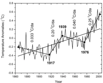
(2003). Figure 3 shows the mean Northern hemisphere
tem-perature between 1865 and 2002, together with the linear fit
and the fit with continuous line segments with a minimum
trend change at breakpoints of 0.2
0C/decade and a minimum
of 20 years between breakpoints, except at the end segments
where a minimum length of 5 years is allowed.
The long term change of NH temperature is estimated
as 0.63
0C (0.046
0C/decade), whereas the corresponding
estimate by the proposed fitting method is slight higher at
0.75
0C (0.054
0C/decade). More importantly, the non-linear
fit captures important information on the interdecadal
evo-lution of surface temperature, detecting two cooling
peri-ods (1865-1917 and 1939-1976) and two warming periperi-ods
(1917-1939 and 1976-2002), with a good visual fit to the
data. A remarkable result, in the context of the climate
change debate, is the high trend value in the most recent
warming period (0.25
0C/decade). This results are
compa-rable with those obtained by Karl et al (2000) for the global
world temperature.
Once again, one may conclude that the condition on the
minimum trend change is an important constraint on the
number of breakpoints. For this time series the chosen
win-dow size allows for 7 breakpoints but the conditions of a
minimum trend change of 0.2
0C/decade reduce that
num-ber down to 3 breakpoints. In this case, the solution obtained
for three breakpoints without additional conditions for the
Fig. 3. Fitting of Northern Hemisphere temperature anomaly with continuous line segments. The minimum amount of trend change at breakpoints is 0.20
C/decade, and 20 years is the minimum allowed interval between breakpoints (5 years for end segments).
minimum trend change is not the same as presented in Fig 3,
although it is quite close. The unconstrained set of 4 line
seg-ments that best fits the time series has breakpoints at 1912,
1943 and 1975, with partial trends of −0.043, 0.15, −0.053
and 0.24
0C/decade, respectively. This solution was not
se-lected in the first place because both at 1912 and 1943 the
changes in trend are smaller than 0.2
0C/decade. However,
the two solutions coincide if one chooses a minimum trend
change of 0.15
0C/decade at the breakpoints. In these cases,
slightly different values of breakpoint positions can lead to
a slightly better fit, and the user has to choose the preferred
solution.
3.3 A case with a large number of data points: Hemispheric
Multi-proxy Temperature Reconstructions
The proposed methodology requires a huge computation
time whenever the time series contains a large number of
data points. In those cases, it is possible to make the
prob-lem treatable by carefully subdividing the time series into a
small number of overlapping sub intervals in order to find
the breakpoint positions in the time series. After finding the
breakpoint positions, one only needs to solve the over
de-termined system linear equations (3). It is important that the
beginning of a sub interval coincides with a breakpoint found
in the previous subinterval. Preferably, the breakpoint chosen
for interval boundary should be sufficiently away from the
boundaries and other breakpoints by a distance larger than
the minimum allowed interval.
There are many large geophysical time series that one
could choose as an example to illustrate the above
men-tioned workaround. We will use the historical reconstruction
of the Northern hemisphere temperature by Mann and Jones
(2003).
Fig. 3. Fitting of Northern Hemisphere temperature anomaly with continuous line segments. The minimum amount of trend change at breakpoints is 0.2◦C/decade, and 20 years is the minimum allowed interval between breakpoints (5 years for end segments).
there is still an ample debate about the statistical support for those conclusions. The reason is apparent in Fig. 1, consider-ing the fact that the mean decadal change of the NAO index is quite small in view of its large interannual variability. In Sect. 5 it will be shown that the methodology here proposed can recover partial trends from synthetic series, defined in its simplest sense as monotonous changes over some time interval, in the presence of significant levels of noise. It will also be shown that the critical point in the performance of the method is the location of the breakpoints and that once these are known, the partial trend values are not much affected by the amplitude of noise.
The breakpoints of NAO presented in Figs. 1 and 2 differ slightly from those presented by Tom´e and Miranda (2004) because in that study end effects were not considered. In that study, a change of sign was always imposed at breakpoints but that didn’t affect the solution in this particular case.
The simultaneous imposition of limits for the segment length and for the change in trend at breakpoints seems a sensible way of constraining the fitting. In the case shown, the imposed minimum segment size allowed a maximum of 7 breakpoints, but the condition of minimum trend change reduced it to 4 breakpoints.
3.2 The Northern Hemisphere temperature record
The Climate Research Unit (CRU), University of East An-glia, produces and frequently updates a database of the global temperature that has been the basis of many global warming studies. The data is freely available at http://www.cru.uea. ac.uk/cru/data/ and is described in Jones et al. (1999) and Jones and Moberg (2003). Figure 3 shows the mean Northern hemisphere temperature between 1865 and 2002, together with the linear fit and the fit with continuous line segments
with a minimum trend change at breakpoints of 0.2◦C/decade
and a minimum of 20 years between breakpoints, except at the end segments where a minimum length of 5 years is al-lowed.
The long term change of NH temperature is estimated as
0.63◦C (0.046◦C/decade), whereas the corresponding
esti-mate by the proposed fitting method is slight higher at 0.75◦C
(0.054◦C/decade). More importantly, the non-linear fit
cap-tures important information on the interdecadal evolution of surface temperature, detecting two cooling periods (1865– 1917 and 1939–1976) and two warming periods (1917–1939 and 1976–2002), with a good visual fit to the data. A re-markable result, in the context of the climate change debate, is the high trend value in the most recent warming period
(0.25◦C/decade). This results are comparable with those
ob-tained by Karl et al. (2000) for the global world temperature. Once again, one may conclude that the condition on the minimum trend change is an important constraint on the number of breakpoints. For this time series the chosen win-dow size allows for 7 breakpoints but the conditions of a
minimum trend change of 0.2◦C/decade reduce that number
down to 3 breakpoints. In this case, the solution obtained for three breakpoints without additional conditions for the min-imum trend change is not the same as presented in Fig. 3, although it is quite close. The unconstrained set of 4 line seg-ments that best fits the time series has breakpoints at 1912, 1943 and 1975, with partial trends of −0.043, 0.15, −0.053
and 0.24◦C/decade, respectively. This solution was not
se-lected in the first place because both at 1912 and 1943 the
changes in trend are smaller than 0.2◦C/decade. However,
the two solutions coincide if one chooses a minimum trend
change of 0.15◦C/decade at the breakpoints. In these cases,
slightly different values of breakpoint positions can lead to a slightly better fit, and the user has to choose the preferred solution.
3.3 A case with a large number of data points: Hemispheric
multi-proxy temperature reconstructions
The proposed methodology requires a huge computation time whenever the time series contains a large number of data points. In those cases, it is possible to make the prob-lem treatable by carefully subdividing the time series into a small number of overlapping sub intervals in order to find the breakpoint positions in the time series. After finding the breakpoint positions, one only needs to solve the over de-termined system linear equations (3). It is important that the beginning of a sub interval coincides with a breakpoint found in the previous subinterval. Preferably, the breakpoint chosen for interval boundary should be sufficiently away from the boundaries and other breakpoints by a distance larger than the minimum allowed interval.
There are many large geophysical time series that one could choose as an example to illustrate the above men-tioned workaround. We will use the historical reconstruction of the Northern hemisphere temperature by Mann and Jones (2003).
A. R. Tom´e and P. M. A. Miranda: Continuous partial trends 455
A. R. Tom´e and P. M. A. Miranda: Continuous Partial Trends
5
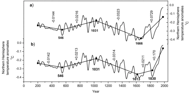
Fig. 4. Fitting of the Northern Hemispheric temperature anomalies, based on 1961-1990 instrumental reference period, with continuous line segments. (a) 200 years minimum distance between breakpoints, and change of trend sign at breakpoints. (b) As (a), but the last interval was allowed to have a minimum length of 150 years and the change in trend at breakpoints is not less than 300%.
Figure 4(a) presents a fit to a series of 1781
years of hemispheric multi-proxy temperature
evalu-ated by Mann and Jones
(2003), freely available at
ftp://ftp.ngdc.noaa.gov/paleo. In this case, the
best fit was obtained, for a condition of change in the trend
sign at breakpoints and a minimum of 200 years between
breakpoints, with breakpoints at the years of 546, 1031 and
1666 AD. The preprocessing of the time series in 3
sub-intervals led to a reduction of computing time by a factor
of 10
6(from almost half a century, virtually impracticable in
a single computer, to less than half and hour in a Pentium IV
PC).
The best fit of the proxy temperature data estimates a
de-crease of the mean temperature in the first 346 years (200 till
546 ac.) at a rate of −0.014
0C/century, followed by a
tem-perature increase at a rate of 0.022
0C/century until 1031,
then a very long period, more than 6 centuries, of
contin-uous temperature decrease at a rate of −0.032
0C/century.
The large rate of warming after 1666, 0.073
0C/century, has
already been able to compensate the previous 6 centuries of
cooling and the last segment attains temperature values above
the local maximum at 1031, at the centre of the warm
me-dieval period AD 800-1400 (Mann and Jones (2003)).
In spite of the relatively good overall fit presented in
fig-ure 4(a), the large single oscillation present in the end of the
proxy temperature time series suggests that one may be
un-derestimating the latter partial trend, due to an end effect
re-lated with the minimum of 200 years of trend duration. Fig.
4(b) presents an alternative fit of the same data of Fig. 4(a)
with the following modification of the optimization
condi-tions: sign change or a minimum relative variation of 300%
in the trend value is imposed at the breakpoints, and a
min-imum length of 150 years is allowed for the last line
seg-ment. The main difference from the result in Fig. 4(a) is
a last trend beginning at 1830 at a faster warming rate of
0.17
0C/century, much higher than elsewhere in the series,
but still below estimates based on thermometer data in the
last century.
4 A spatial aggregation technique
The proposed methodology is clearly a univariate time series
analysis technique. However, it defines for a given time
se-ries a new set of parameters, the breakpoints, that can be used
to perform spatial aggregation of a time varying field. The
idea was proposed by Miranda and Tom´e (2005) and applied
to the NASA/GISS surface temperature dataset (Hansen et al
(1999)), leading to the conclusion that the spatial
distribu-tion of the temperature breakpoints in the last 50 years is a
coherent large scale field, that may be relevant for the
under-standing of the slow evolution of the climate system in that
period.
To illustrate the potential use of the method as a
spa-tial analysis tool we will apply it to a different climate
database, namely the NCEP/NCAR 2m reanalysis
temper-ature (Kalnay et al (1996)), available from 1950 onwards
and obtained through the assimilation of meteorological
ob-servations by a state of the art numerical weather prediction
model. Reanalysis data has been used for climate change
studies (Kalnay and Cai (2003)) but is generally discarded
Fig. 4. Fitting of the Northern Hemispheric temperature anomalies, based on 1961-1990 instrumental reference period, with continuous line segments. (a) 200 years minimum distance between breakpoints, and change of trend sign at breakpoints. (b) As (a), but the last interval was allowed to have a minimum length of 150 years and the change in trend at breakpoints is not less than 300%.
Figure 4a presents a fit to a series of 1781 years of hemispheric multi-proxy temperature evaluated by Mann and Jones (2003), freely available at ftp://ftp.ngdc.noaa.gov/ paleo. In this case, the best fit was obtained, for a condition of change in the trend sign at breakpoints and a minimum of 200 years between breakpoints, with breakpoints at the years of 546, 1031 and 1666 AD. The preprocessing of the time series in 3 sub-intervals led to a reduction of computing time by a factor of 106(from almost half a century, virtually im-practicable in a single computer, to less than half and hour in a Pentium IV PC).
The best fit of the proxy temperature data estimates a de-crease of the mean temperature in the first 346 years (200
till 546 ac.) at a rate of −0.014◦C/century, followed by a
temperature increase at a rate of 0.022◦C/century until 1031, then a very long period, more than 6 centuries, of
continu-ous temperature decrease at a rate of −0.032◦C/century. The
large rate of warming after 1666, 0.073◦C/century, has
al-ready been able to compensate the previous 6 centuries of cooling and the last segment attains temperature values above the local maximum at 1031, at the centre of the warm me-dieval period AD 800–1400 (Mann and Jones, 2003).
In spite of the relatively good overall fit presented in Fig. 4a, the large single oscillation present in the end of the proxy temperature time series suggests that one may be un-derestimating the latter partial trend, due to an end effect re-lated with the minimum of 200 years of trend duration. Fig-ure 4b presents an alternative fit of the same data of Fig. 4a with the following modification of the optimization condi-tions: sign change or a minimum relative variation of 300% in the trend value is imposed at the breakpoints, and a mini-mum length of 150 years is allowed for the last line segment. The main difference from the result in Fig. 4a is a last trend
beginning at 1830 at a faster warming rate of 0.17◦C/century, much higher than elsewhere in the series, but still below es-timates based on thermometer data in the last century.
4 A spatial aggregation technique
The proposed methodology is clearly a univariate time series analysis technique. However, it defines for a given time se-ries a new set of parameters, the breakpoints, that can be used to perform spatial aggregation of a time varying field. The idea was proposed by Miranda and Tom´e (2005) and applied to the NASA/GISS surface temperature dataset (Hansen et al., 1999), leading to the conclusion that the spatial distribu-tion of the temperature breakpoints in the last 50 years is a coherent large scale field, that may be relevant for the under-standing of the slow evolution of the climate system in that period.
To illustrate the potential use of the method as a spa-tial analysis tool we will apply it to a different climate database, namely the NCEP/NCAR 2 m reanalysis temper-ature (Kalnay et al., 1996), available from 1950 onwards and obtained through the assimilation of meteorological obser-vations by a state of the art numerical weather prediction model. Reanalysis data has been used for climate change studies (Kalnay and Cai, 2003) but is generally discarded for this application because of time dependent biases in the data that is used by reanalysis, namely in what concerns satellite data (Basist and Chelliah, 1997; Hurrell and Trenberth, 1998; Santer et al., 1999, 2000; Stendel et al., 2000). However, it is ideally suited for our current purpose as it has a global cov-erage, without the missing data that often hinders the use of direct observations.
456 A. R. Tom´e and P. M. A. Miranda: Continuous partial trends
6 A. R. Tom´e and P. M. A. Miranda: Continuous Partial Trends
180˚ 180˚ 150˚W 150˚W 120˚W 120˚W 90˚W 90˚W 60˚W 60˚W 30˚W 30˚W 0˚ 0˚ 0˚ 0˚ 30˚N 30˚N 60˚N 60˚N 90˚N 90˚N 1950 1960 1970 1980 1990 1995 180˚ 180˚ 150˚W 150˚W 120˚W 120˚W 90˚W 90˚W 60˚W 60˚W 30˚W 30˚W 0˚ 0˚ 0˚ 0˚ 30˚N 30˚N 60˚N 60˚N 90˚N 90˚N
Fig. 5. year of change in sign of local temperature tendency. Blank in regions with no breakpoint.
for this application because of time dependent biases in the data that is used by reanalysis, namely in what concerns satellite data (Basist and Chelliah (1997), Hurrell and Tren-berth (1998), Santer et al (1999), (2000), Stendel et al (2000)). However, it is ideally suited for our current pur-pose as it has a global coverage, without the missing data that often hinders the use of direct observations.
Considering the evolution of mean world temperature one would expect one single breakpoint in the period 1950-2002 with a cooling period followed by warming. For mean world temperature that breakpoint should be around 1975 as shown by Karl et al (2000). However, a point by point analysis of the reanalysis time series shows that the breakpoint year varies from place to place in a rather consistent way. Figure 5 shows the breakpoint distribution in the North American gion, from a best fit of the NCEP/NCAR 2m temperature re-analysis field where only two line segments are allowed and a change in trend sign is imposed at the breakpoint. White regions in the figure are places of monotonous temperature change, mostly sustained warming, where a breakpoint with a trend sign change cannot be defined. Ten years was the minimum allowed length for each of the sub intervals.
The North American region is where we find a larger dis-crepancy between estimates of long term change in temper-ature given by a linear trend without breakpoint and by the linear trend with one breakpoint. In this region, the linear trend gives, in some places, strong negative values that are not supported by the integrated segments, as the linear fit in the temperature time series is obviously inadequate.
Fig. 6 presents the net change in temperature in the North American region, estimated by linear regression and by the integration of the two fitted segments. While the simple lin-ear fit leads to large net cooling, especially over Greenland and Baffin Bay and in a large sector of the USA territory, the broken line approach suggests moderate net cooling in most places, with recent warming compensating for previous cooling in many regions, namely in half of Greenland.
An important feature of the breakpoint map shown in Fig. 5 is the fact that the observed breakpoints span the entire four decades range in a spatially consistent way, as one could
180˚ 180˚ 150˚W 150˚W 120˚W 120˚W 90˚W 90˚W 60˚W 60˚W 30˚W 30˚W 0˚ 0˚ 0˚ 0˚ 30˚N 30˚N 60˚N 60˚N 90˚N 90˚N -10.0 -5.0 -4.0 -3.0 -2.0 -1.0 -0.5 0.0 0.5 1.0 2.0 3.0 4.0 5.0 10.0 180˚ 180˚ 150˚W 150˚W 120˚W 120˚W 90˚W 90˚W 60˚W 60˚W 30˚W 30˚W 0˚ 0˚ 0˚ 0˚ 30˚N 30˚N 60˚N 60˚N 90˚N 90˚N 180˚ 180˚ 150˚W 150˚W 120˚W 120˚W 90˚W 90˚W 60˚W 60˚W 30˚W 30˚W 0˚ 0˚ 0˚ 0˚ 30˚N 30˚N 60˚N 60˚N 90˚N 90˚N -10.0 -5.0 -4.0 -3.0 -2.0 -1.0 -0.5 0.0 0.5 1.0 2.0 3.0 4.0 5.0 10.0 180˚ 180˚ 150˚W 150˚W 120˚W 120˚W 90˚W 90˚W 60˚W 60˚W 30˚W 30˚W 0˚ 0˚ 0˚ 0˚ 30˚N 30˚N 60˚N 60˚N 90˚N 90˚N
Fig. 6. Temperature variation of the mean surface temperature, in 0
C: upper figure linear variation, lower figure two continuous line best fit
expected by the spatial correlation of the reanalysis fields. However, Miranda and Tom´e (2005) obtained a similar pat-tern with GISS data and suggested that this is a signature of a slow evolution of the climate heat transfer engine in the region, associated with the NAO evolution in the same pe-riod. The spatial coherency of the breakpoint distribution, with neighboring grid points experiencing similar tempera-ture changes, also suggests the spatial aggregation of regions with similar breakpoint locations, as done by Miranda and Tom´e (2005). Other time varying geophysical fields may be analyzed with the same methodology.
5 Statistical Significance
An important and unavoidable issue is the statistical signif-icance of the breakpoints and/or the partial trends. At first glance, one may be tempted to test the individual partial trends for significance using some of the many techniques that have been proposed by several authors in the last decades (e.g. Gordon (1991), Bloomfield (1992), Bloomfield and Nychka (1992), Visser and Molenaar (1995), Zheng et al. (1997)) and consider as statistical significant those results above a given threshold of the confidence interval. However, in spite of the huge effort put in the analysis of the signifi-cance of the simple linear trend model, a simple and objec-tive method has not yet obtained general consensus, and the different models lead to different conclusions, not just in the
Fig. 5. Year of change in sign of local temperature tendency. Blank in regions with no breakpoint.
Considering the evolution of mean world temperature one would expect one single breakpoint in the period 1950–2002 with a cooling period followed by warming. For mean world temperature that breakpoint should be around 1975 as shown by (Karl et al., 2000). However, a point by point analysis of the reanalysis time series shows that the breakpoint year varies from place to place in a rather consistent way. Figure 5 shows the breakpoint distribution in the North American gion, from a best fit of the NCEP/NCAR 2m temperature re-analysis field where only two line segments are allowed and a change in trend sign is imposed at the breakpoint. White regions in the figure are places of monotonous temperature change, mostly sustained warming, where a breakpoint with a trend sign change cannot be defined. Ten years was the minimum allowed length for each of the sub intervals.
The North American region is where we find a larger dis-crepancy between estimates of long term change in temper-ature given by a linear trend without breakpoint and by the linear trend with one breakpoint. In this region, the linear trend gives, in some places, strong negative values that are not supported by the integrated segments, as the linear fit in the temperature time series is obviously inadequate.
Figure 6 presents the net change in temperature in the North American region, estimated by linear regression and by the integration of the two fitted segments. While the sim-ple linear fit leads to large net cooling, especially over Green-land and Baffin Bay and in a large sector of the USA territory, the broken line approach suggests moderate net cooling in most places, with recent warming compensating for previous cooling in many regions, namely in half of Greenland.
An important feature of the breakpoint map shown in Fig. 5 is the fact that the observed breakpoints span the entire four decades range in a spatially consistent way, as one could expected by the spatial correlation of the reanalysis fields. However, Miranda and Tom´e (2005) obtained a similar pat-tern with GISS data and suggested that this is a signature of a slow evolution of the climate heat transfer engine in the region, associated with the NAO evolution in the same pe-riod. The spatial coherency of the breakpoint distribution, with neighboring grid points experiencing similar
tempera-6 A. R. Tom´e and P. M. A. Miranda: Continuous Partial Trends
180˚ 180˚ 150˚W 150˚W 120˚W 120˚W 90˚W 90˚W 60˚W 60˚W 30˚W 30˚W 0˚ 0˚ 0˚ 0˚ 30˚N 30˚N 60˚N 60˚N 90˚N 90˚N 1950 1960 1970 1980 1990 1995 180˚ 180˚ 150˚W 150˚W 120˚W 120˚W 90˚W 90˚W 60˚W 60˚W 30˚W 30˚W 0˚ 0˚ 0˚ 0˚ 30˚N 30˚N 60˚N 60˚N 90˚N 90˚N
Fig. 5. year of change in sign of local temperature tendency. Blank in regions with no breakpoint.
for this application because of time dependent biases in the data that is used by reanalysis, namely in what concerns satellite data (Basist and Chelliah (1997), Hurrell and Tren-berth (1998), Santer et al (1999), (2000), Stendel et al (2000)). However, it is ideally suited for our current pur-pose as it has a global coverage, without the missing data that often hinders the use of direct observations.
Considering the evolution of mean world temperature one would expect one single breakpoint in the period 1950-2002 with a cooling period followed by warming. For mean world temperature that breakpoint should be around 1975 as shown by Karl et al (2000). However, a point by point analysis of the reanalysis time series shows that the breakpoint year varies from place to place in a rather consistent way. Figure 5 shows the breakpoint distribution in the North American gion, from a best fit of the NCEP/NCAR 2m temperature re-analysis field where only two line segments are allowed and a change in trend sign is imposed at the breakpoint. White regions in the figure are places of monotonous temperature change, mostly sustained warming, where a breakpoint with a trend sign change cannot be defined. Ten years was the minimum allowed length for each of the sub intervals.
The North American region is where we find a larger dis-crepancy between estimates of long term change in temper-ature given by a linear trend without breakpoint and by the linear trend with one breakpoint. In this region, the linear trend gives, in some places, strong negative values that are not supported by the integrated segments, as the linear fit in the temperature time series is obviously inadequate.
Fig. 6 presents the net change in temperature in the North American region, estimated by linear regression and by the integration of the two fitted segments. While the simple lin-ear fit leads to large net cooling, especially over Greenland and Baffin Bay and in a large sector of the USA territory, the broken line approach suggests moderate net cooling in most places, with recent warming compensating for previous cooling in many regions, namely in half of Greenland.
An important feature of the breakpoint map shown in Fig. 5 is the fact that the observed breakpoints span the entire four decades range in a spatially consistent way, as one could
180˚ 180˚ 150˚W 150˚W 120˚W 120˚W 90˚W 90˚W 60˚W 60˚W 30˚W 30˚W 0˚ 0˚ 0˚ 0˚ 30˚N 30˚N 60˚N 60˚N 90˚N 90˚N -10.0 -5.0 -4.0 -3.0 -2.0 -1.0 -0.5 0.0 0.5 1.0 2.0 3.0 4.0 5.0 10.0 180˚ 180˚ 150˚W 150˚W 120˚W 120˚W 90˚W 90˚W 60˚W 60˚W 30˚W 30˚W 0˚ 0˚ 0˚ 0˚ 30˚N 30˚N 60˚N 60˚N 90˚N 90˚N 180˚ 180˚ 150˚W 150˚W 120˚W 120˚W 90˚W 90˚W 60˚W 60˚W 30˚W 30˚W 0˚ 0˚ 0˚ 0˚ 30˚N 30˚N 60˚N 60˚N 90˚N 90˚N -10.0 -5.0 -4.0 -3.0 -2.0 -1.0 -0.5 0.0 0.5 1.0 2.0 3.0 4.0 5.0 10.0 180˚ 180˚ 150˚W 150˚W 120˚W 120˚W 90˚W 90˚W 60˚W 60˚W 30˚W 30˚W 0˚ 0˚ 0˚ 0˚ 30˚N 30˚N 60˚N 60˚N 90˚N 90˚N
Fig. 6. Temperature variation of the mean surface temperature, in 0
C: upper figure linear variation, lower figure two continuous line best fit
expected by the spatial correlation of the reanalysis fields. However, Miranda and Tom´e (2005) obtained a similar pat-tern with GISS data and suggested that this is a signature of a slow evolution of the climate heat transfer engine in the region, associated with the NAO evolution in the same pe-riod. The spatial coherency of the breakpoint distribution, with neighboring grid points experiencing similar tempera-ture changes, also suggests the spatial aggregation of regions with similar breakpoint locations, as done by Miranda and Tom´e (2005). Other time varying geophysical fields may be analyzed with the same methodology.
5 Statistical Significance
An important and unavoidable issue is the statistical signif-icance of the breakpoints and/or the partial trends. At first glance, one may be tempted to test the individual partial trends for significance using some of the many techniques that have been proposed by several authors in the last decades (e.g. Gordon (1991), Bloomfield (1992), Bloomfield and Nychka (1992), Visser and Molenaar (1995), Zheng et al. (1997)) and consider as statistical significant those results above a given threshold of the confidence interval. However, in spite of the huge effort put in the analysis of the signifi-cance of the simple linear trend model, a simple and objec-tive method has not yet obtained general consensus, and the different models lead to different conclusions, not just in the
Fig. 6. Temperature variation of the mean surface temperature, in
◦C: upper figure linear variation, lower figure two continuous line best fit.
ture changes, also suggests the spatial aggregation of regions with similar breakpoint locations, as done by Miranda and Tom´e (2005). Other time varying geophysical fields may be analyzed with the same methodology.
5 Statistical significance
An important and unavoidable issue is the statistical signif-icance of the breakpoints and/or the partial trends. At first glance, one may be tempted to test the individual partial trends for significance using some of the many techniques that have been proposed by several authors in the last decades (e.g. Gordon, 1991; Bloomfield, 1992; Bloomfield and Ny-chka, 1992; Visser and Molenaar, 1995; Zheng et al., 1997) and consider as statistical significant those results above a given threshold of the confidence interval. However, in spite of the huge effort put in the analysis of the significance of the simple linear trend model, a simple and objective method has not yet obtained general consensus, and the different models lead to different conclusions, not just in the value and statisti-cal significance of a trend, but also in the validity of the trend model itself.
Karl et al. (2000) applied standard significance tests to dis-cuss the trend computed for the last segment in a broken-line fitting of the mean world temperature. It is not possible to extend that approach to the full problem, which includes the computation of the number of breakpoints, its location and
A. R. Tom´e and P. M. A. Miranda: Continuous partial trends 457
A. R. Tom´e and P. M. A. Miranda: Continuous Partial Trends
7
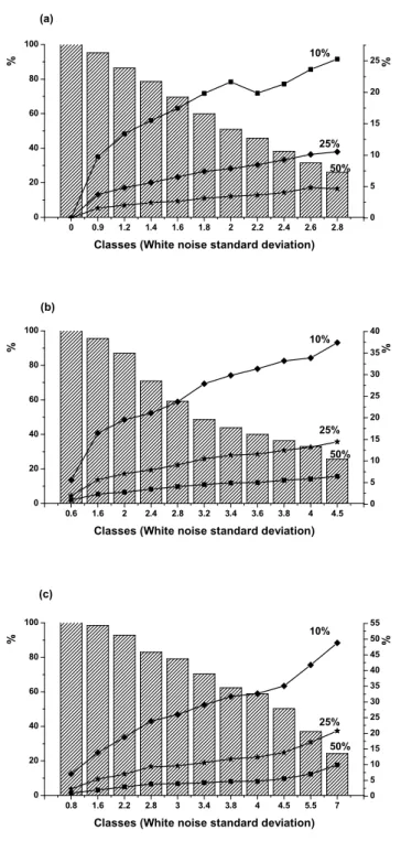
Fig. 7. Performance of the broken-line fitting as a function of the error level. Bars (left axis): Percentage of breakpoints recovered without error. Lines (right axis): Frequency of errors in the partial trends above different thresholds, for the cases where the breakpoint inversion was successful. The level of noise (low axis) is given by the standard deviation of the white noise.
value and statistical significance of a trend, but also in the
validity of the trend model itself.
Karl et al (2000) applied standard significance tests to
dis-cuss the trend computed for the last segment in a broken-line
fitting of the mean world temperature. It is not possible to
extend that approach to the full problem, which includes the
computation of the number of breakpoints, its location and
the evaluation of partial trends, with a condition of continuity
of the fitting function at the breakpoints. If, as in the case of
DFA (Peng et al (1994)), one specifies the subinterval range
and then applies unconstrained linear fit, without a condition
of continuity at the subinterval boundaries, one could test for
the individual significance of each of the individual partial
trends. Yet, in that case, one should be aware of the biased
conclusions on significance due to the sub interval chosen,
because in that particular case the warnings about the
signifi-cance of the trend value formulated by Percival and Rothrock
(2005) are especially pertinent and should be taken into
ac-count.
While a general test is difficult to obtain, one can easily
check the ability of the proposed method to cope with the
difficulties of real data, by the analysis of a large number of
simulations with synthetic time series. For that purpose we
have computed 10000 non-dimensional time series, of 100
data points each, made of random continuous line segments
with a minimum length of 15 data points and a minimum
change in trend of 0.1/datapoint at breakpoints. The trend
values were in the range [0,1]/datapoint. With these
condi-tions the random series could have at most 6 line segments
(5 breakpoints). Situations with only one line segment (zero
breakpoints) were also allowed. As expected, the method
was able to recover all the breakpoints (or its absence) and
corresponding trend values from this series. In the next step
we added to these random series white noise of varying
am-plitude.
Figure 7 shows the results of the inversion of the 10000
Fig. 8. Results of the inversion of one of the series used in figure 7 for different noise levels.
random series, for different values of the noise level. When
there is no noise, the inversion works at 100%, recovering
all breakpoints at the right location and computing all partial
trends at round-off error. In the presence of significant noise
(with standard deviations from 0.5 to 1.8 in non-dimensional
units) the frequency of misfits increases steadily with the
noise level, as shown in the figure. However, for the
frac-tion of cases where the breakpoints were found within 2
dat-apoints of their right location, which are considered to have
been well located, the maximum relative error in the partial
trends remains within reasonable bounds, even when the
er-ror level is such that the fraction of misfits is above 50%.
This means that if the breakpoint location is known the
par-tial trends are not too sensitive to the noise. On the other
hand, most of the cases that present larger relative errors in
the partial trends happen in the last segment, because it is the
least constrained.
Figure 8 shows an example of the inversion of a series with
1 breakpoint, taken from the set used in figure 7. The top line
corresponds to the series without any added noise, which is
perfectly inverted. The series with 0.7 and 1.0 noise also lead
to successful inversions, in spite of the large random
oscilla-tions present in the series. However, when the noise standard
deviation attains 1.6, the method proposes the maximum
al-lowed number of breakpoints. An eye inspection of this
re-sult suggests, though, that the proposed fitting is not at all
unrealistic.
Fig. 7. Performance of the broken-line fitting as a function of the error level. Bars (left axis): Percentage of breakpoints recovered without error. Lines (right axis): Frequency of errors in the partial trends above different thresholds, for the cases where the breakpoint inversion was successful. The level of noise (low axis) is given by the standard deviation of the white noise.
the evaluation of partial trends, with a condition of continu-ity of the fitting function at the breakpoints. If, as in the case of DFA (Peng et al., 1994), one specifies the subinter-val range and then applies unconstrained linear fit, without a condition of continuity at the subinterval boundaries, one could test for the individual significance of each of the indi-vidual partial trends. Yet, in that case, one should be aware of the biased conclusions on significance due to the sub inter-val chosen, because in that particular case the warnings about the significance of the trend value formulated by Percival and Rothrock (2005) are especially pertinent and should be taken into account.
While a general test is difficult to obtain, one can easily check the ability of the proposed method to cope with the difficulties of real data, by the analysis of a large number of simulations with synthetic time series. For that purpose we have computed 10 000 non-dimensional time series, of 100 data points each, made of random continuous line segments with a minimum length of 15 data points and a minimum change in trend of 0.1/datapoint at breakpoints. The trend values were in the range [0,1]/datapoint. With these condi-tions the random series could have at most 6 line segments (5 breakpoints). Situations with only one line segment (zero breakpoints) were also allowed. As expected, the method was able to recover all the breakpoints (or its absence) and corresponding trend values from this series. In the next step we added to these random series white noise of varying am-plitude.
Figure 7 shows the results of the inversion of the 10 000 random series, for different values of the noise level. When there is no noise, the inversion works at 100%, recovering all breakpoints at the right location and computing all partial trends at round-off error. In the presence of significant noise (with standard deviations from 0.5 to 1.8 in non-dimensional units) the frequency of misfits increases steadily with the noise level, as shown in the figure. However, for the frac-tion of cases where the breakpoints were found within 2
dat-A. R. Tom´e and P. M. dat-A. Miranda: Continuous Partial Trends
7
Fig. 7. Performance of the broken-line fitting as a function of the error level. Bars (left axis): Percentage of breakpoints recovered without error. Lines (right axis): Frequency of errors in the partial trends above different thresholds, for the cases where the breakpoint inversion was successful. The level of noise (low axis) is given by the standard deviation of the white noise.
value and statistical significance of a trend, but also in the
validity of the trend model itself.
Karl et al (2000) applied standard significance tests to
dis-cuss the trend computed for the last segment in a broken-line
fitting of the mean world temperature. It is not possible to
extend that approach to the full problem, which includes the
computation of the number of breakpoints, its location and
the evaluation of partial trends, with a condition of continuity
of the fitting function at the breakpoints. If, as in the case of
DFA (Peng et al (1994)), one specifies the subinterval range
and then applies unconstrained linear fit, without a condition
of continuity at the subinterval boundaries, one could test for
the individual significance of each of the individual partial
trends. Yet, in that case, one should be aware of the biased
conclusions on significance due to the sub interval chosen,
because in that particular case the warnings about the
signifi-cance of the trend value formulated by Percival and Rothrock
(2005) are especially pertinent and should be taken into
ac-count.
While a general test is difficult to obtain, one can easily
check the ability of the proposed method to cope with the
difficulties of real data, by the analysis of a large number of
simulations with synthetic time series. For that purpose we
have computed 10000 non-dimensional time series, of 100
data points each, made of random continuous line segments
with a minimum length of 15 data points and a minimum
change in trend of 0.1/datapoint at breakpoints. The trend
values were in the range [0,1]/datapoint. With these
condi-tions the random series could have at most 6 line segments
(5 breakpoints). Situations with only one line segment (zero
breakpoints) were also allowed. As expected, the method
was able to recover all the breakpoints (or its absence) and
corresponding trend values from this series. In the next step
we added to these random series white noise of varying
am-plitude.
Figure 7 shows the results of the inversion of the 10000
Fig. 8. Results of the inversion of one of the series used in figure 7 for different noise levels.
random series, for different values of the noise level. When
there is no noise, the inversion works at 100%, recovering
all breakpoints at the right location and computing all partial
trends at round-off error. In the presence of significant noise
(with standard deviations from 0.5 to 1.8 in non-dimensional
units) the frequency of misfits increases steadily with the
noise level, as shown in the figure. However, for the
frac-tion of cases where the breakpoints were found within 2
dat-apoints of their right location, which are considered to have
been well located, the maximum relative error in the partial
trends remains within reasonable bounds, even when the
er-ror level is such that the fraction of misfits is above 50%.
This means that if the breakpoint location is known the
par-tial trends are not too sensitive to the noise. On the other
hand, most of the cases that present larger relative errors in
the partial trends happen in the last segment, because it is the
least constrained.
Figure 8 shows an example of the inversion of a series with
1 breakpoint, taken from the set used in figure 7. The top line
corresponds to the series without any added noise, which is
perfectly inverted. The series with 0.7 and 1.0 noise also lead
to successful inversions, in spite of the large random
oscilla-tions present in the series. However, when the noise standard
deviation attains 1.6, the method proposes the maximum
al-lowed number of breakpoints. An eye inspection of this
re-sult suggests, though, that the proposed fitting is not at all
unrealistic.
Fig. 8. Results of the inversion of one of the series used in Fig. 7 for different noise levels.
apoints of their right location, which are considered to have been well located, the maximum relative error in the partial trends remains within reasonable bounds, even when the er-ror level is such that the fraction of misfits is above 50%. This means that if the breakpoint location is known the par-tial trends are not too sensitive to the noise. On the other hand, most of the cases that present larger relative errors in the partial trends happen in the last segment, because it is the least constrained.
Figure 8 shows an example of the inversion of a series with 1 breakpoint, taken from the set used in Fig. 7. The top line corresponds to the series without any added noise, which is perfectly inverted. The series with 0.7 and 1.0 noise also lead to successful inversions, in spite of the large random oscilla-tions present in the series. However, when the noise standard deviation attains 1.6, the method proposes the maximum al-lowed number of breakpoints. An eye inspection of this re-sult suggests, though, that the proposed fitting is not at all unrealistic.
The random series considered in Fig. 7 were rather dif-ficult to invert due to the small relative size of its shorter line segments and the small changes of trend allowed at each breakpoint. If either of these parameters is increased, the method is able to cope with much larger noise levels. Fig-ure 9 shows the results of 3 other sets of 10 000 random se-ries, similar to those used in Fig. 7 but with at least 20, 25 and 30 datapoints per segment, respectively. As the