HAL Id: hal-00296129
https://hal.archives-ouvertes.fr/hal-00296129
Submitted on 25 Jan 2007
HAL is a multi-disciplinary open access
archive for the deposit and dissemination of
sci-entific research documents, whether they are
pub-lished or not. The documents may come from
teaching and research institutions in France or
abroad, or from public or private research centers.
L’archive ouverte pluridisciplinaire HAL, est
destinée au dépôt et à la diffusion de documents
scientifiques de niveau recherche, publiés ou non,
émanant des établissements d’enseignement et de
recherche français ou étrangers, des laboratoires
publics ou privés.
Persistence and photochemical decay of springtime total
ozone anomalies in the Canadian Middle Atmosphere
Model
S. Tegtmeier, T. G. Shepherd
To cite this version:
S. Tegtmeier, T. G. Shepherd. Persistence and photochemical decay of springtime total ozone
anoma-lies in the Canadian Middle Atmosphere Model. Atmospheric Chemistry and Physics, European
Geosciences Union, 2007, 7 (2), pp.485-493. �hal-00296129�
www.atmos-chem-phys.net/7/485/2007/ © Author(s) 2007. This work is licensed under a Creative Commons License.
Chemistry
and Physics
Persistence and photochemical decay of springtime total ozone
anomalies in the Canadian Middle Atmosphere Model
S. Tegtmeier1,*and T. G. Shepherd2
1Alfred Wegener Institute for Polar and Marine Research, Potsdam, Germany 2Department of Physics, University of Toronto, Toronto, Ontario, Canada *now at: Department of Physics, University of Toronto, Canada
Received: 19 January 2006 – Published in Atmos. Chem. Phys. Discuss.: 28 April 2006 Revised: 19 December 2006 – Accepted: 21 December 2006 – Published: 25 January 2007
Abstract. The persistence and decay of springtime total ozone anomalies over the entire extratropics (midlatitudes plus polar regions) is analysed using results from the Cana-dian Middle Atmosphere Model (CMAM), a comprehensive chemistry-climate model. As in the observations, interan-nual anomalies established through winter and spring persist with very high correlation coefficients (above 0.8) through summer until early autumn, while decaying in amplitude as a result of photochemical relaxation in the quiescent summer-time stratosphere. The persistence and decay of the ozone anomalies in CMAM agrees extremely well with observa-tions, even in the southern hemisphere when the model is run without heterogeneous chemistry (in which case there is no ozone hole and the seasonal cycle of ozone is quite different from observations). However in a version of CMAM with strong vertical diffusion, the northern hemisphere anomalies decay far too rapidly compared to observations. This shows that ozone anomaly persistence and decay does not depend on how the springtime anomalies are created or on their mag-nitude, but reflects the transport and photochemical decay in the model. The seasonality of the long-term trends over the entire extratropics is found to be explained by the persistence of the interannual anomalies, as in the observations, demon-strating that summertime ozone trends reflect winter/spring trends rather than any change in summertime ozone chem-istry. However this mechanism fails in the northern hemi-sphere midlatitudes because of the relatively large impact, compared to observations, of the CMAM polar anomalies. As in the southern hemisphere, the influence of polar ozone loss in CMAM increases the midlatitude summertime loss, leading to a relatively weak seasonal dependence of ozone loss in the Northern Hemisphere compared to the observa-tions.
Correspondence to: S. Tegtmeier (susann@atmosp.physics.utoronto.ca)
1 Introduction
Fioletov and Shepherd (2003, hereinafter referred to as F&S 2003) showed that interannual total ozone anomalies in mid-latitudes develop through the winter and spring, and then persist through summer until autumn. Weber et al. (2003) showed that these anomalies (in both spring and late sum-mer) are related to anomalies in the dynamical forcing of the Brewer-Dobson circulation. During winter and early spring there is a buildup of ozone which is caused by the domi-nance of transport processes during this period. This buildup is followed by a decline through late spring and summer when transport becomes less important and photochemical loss controls the time evolution of midlatitude total ozone. During this summertime period of total ozone decline the ozone anomalies decrease in magnitude through photochem-ical relaxation, and then are rapidly erased when the next winter’s buildup begins. In general the persistence of the midlatitude ozone anomalies is stronger in the northern hemi-sphere (NH) than in the southern hemihemi-sphere (SH). This is due to the influence of springtime polar ozone depletion on midlatitude ozone after the breakup of the vortex. Fioletov & Shepherd (2005, hereinafter referred to as F&S 2005) went on to show that the persistence of the total ozone anomalies is much greater in the SH when the entire extratropics (35◦S–
80◦S) is included, since the region is then not sensitive to
transport across 60◦S. (The region poleward of 80◦latitude
is not observed by TOMS or SBUV, but because of the very small area involved contributes very little to the entire extra-tropical amounts.)
These observed relationships provide a valuable diagnos-tic for process-oriented model validation. The F&S 2003 approach is used here to compare the persistence and pho-tochemical decay of total ozone anomalies in the Canadian Middle Atmosphere Model (CMAM) with observations.
486 S. Tegtmeier and T. G. Shepherd: Ozone anomalies in CMAM
Apr May Jun Jul Aug Sep Oct Nov Dec Jan Feb Mar 260 280 300 320 340 360 380 35°S − 60°S d)
Total Ozone [DU]
CMAM
Apr May Jun Jul Aug Sep Oct Nov Dec Jan Feb Mar 260 280 300 320 340 360 380 35°S − 60°S a)
Total Ozone [DU]
TOMS & SBUV
Apr May Jun Jul Aug Sep Oct Nov Dec Jan Feb Mar 150 200 250 300 350 400 60°S − 80°S e)
Total Ozone [DU]
Apr May Jun Jul Aug Sep Oct Nov Dec Jan Feb Mar 150 200 250 300 350 400 60°S − 80°S b)
Total Ozone [DU]
Apr May Jun Jul Aug Sep Oct Nov Dec Jan Feb Mar 260 280 300 320 340 360 380 35°S − 80°S f)
Total Ozone [DU]
Apr May Jun Jul Aug Sep Oct Nov Dec Jan Feb Mar 260 280 300 320 340 360 380 35°S − 80°S c)
Total Ozone [DU]
Fig. 1. Seasonal cycle of area weighted total ozone values averaged over SH midlatitudes (35◦S–60◦S), polar latitudes (60◦S–80◦S), and the entire extratropical region (35◦S–80◦S), for the merged TOMS & SBUV data set on the left hand side and for CMAM on the right hand
side. Each curve corresponds to a different year. The values are the anomalies from the long term trend added to the EESC fit for the year 2000.
2 Data sets and methodology
We use the same version of the merged satellite data set as in F&S 2005. The set is prepared by NASA and combines version 8 of the TOMS and SBUV data for the time period from November 1978 to December 2003 (Frith et al., 2004). The zonal mean total ozone values cover up to 80◦N from
April to September in the NH and up to 80◦S from October
to March in the SH. The data for August and September 1995 as well as May and June 1996 are missing. We use estimates of total ozone from ground based measurements to fill the gaps (Fioletov et al., 2002). The 24-year time series of each month consists of monthly and zonal means which are area weighted and averaged over certain latitude bands.
The CMAM is a three-dimensional chemistry-climate
model with comprehensive physical parameterisations (Bea-gley et al., 1997; de Grandpr´e et al., 2000). The version used here has a domain from the surface of the earth to approx-imately 97 km and T32 spectral truncation. The model in-cludes a fully interactive stratospheric chemistry with all the relevant catalytic ozone loss cycles and heterogeneous reac-tions for sulphate aerosols, liquid ternary solureac-tions (the so-called Type 1b Polar Stratospheric Clouds, PSCs) and water ice (Type 2 PSCs). There is no parameterisation of nitric acid trihydrate PSCs (Type 1a PSCs) or any associated den-itrification. To calculate the persistence and photochemical decay of total ozone anomalies in CMAM we use ozone data from a 45-year transient run of the model. The run (Eyring et al., 2006) was performed for the period 1960-2004 and was forced by observed changes in well-mixed greenhouse gases,
halogens, and sea-surface temperatures.
The total ozone autocorrelations were calculated for the entire extratropics for both hemispheres (35◦–80◦ latitude)
as a function of time lag for each month of the year. The autocorrelation is thus R(t, τ ) = Pn i=1fi(t )fi(t + τ ) q Pn i=1fi(t )2 q Pn i=1fi(t + τ )2
where n is the number of years in the record, t is a particular month, t + τ is a subsequent month lagged by τ months, and
fi is the deviation from the mean in the year i. The
correla-tion coefficients between ozone values for the same month in different years are low. Thus each year can be considered as independent and correlation coefficients greater than 0.4 are statistically significant at the 95% confidence level for the observations, and greater than 0.3 for CMAM.
As in F&S 2005 we scale the equivalent effective strato-spheric chlorine (EESC) (WMO, 2003) trend to be one unit per year during the 1980s and use the scaled EESC loading as a proxy for the long term trend of each time series. Thus we can express the trend coefficients in DU/year during the 1980s. We remove the EESC fit prior to the anomaly analy-sis.
3 Short-term variations
Figure 1 shows the seasonal cycle of total ozone in the SH from both observations and from CMAM, averaged over 35◦S–60◦S, 60◦S–80◦S and 35◦S–80◦S for each year in
the relevant data sets. The values are the anomalies from the long term trend added to the EESC fit for the year 2000. In this way, the absolute values of the two data sets are directly comparable even though the data sets cover different time pe-riods. The seasonal cycle of total ozone shows a late spring maximum in midlatitudes and a late spring minimum in po-lar regions, the latter reflecting the springtime popo-lar ozone depletion. In autumn CMAM midlatitude ozone levels ex-hibit a positive bias of about 10 DU relative to observations. Furthermore, the seasonal cycle of total ozone for the entire extratropical region is slightly stronger in the observations.
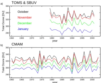
As noted in F&S 2003, the anomalies established in spring appear to persist through the summer. This is illustrated by Fig. 2, which shows the year to year variability of total ozone anomalies averaged over the SH extratropics for the four spring/early summer months for both observations and model. The interannual anomalies are highly correlated from month to month, and the anomalies established in October decrease continuously through January. Since the seasonal cycle of the CMAM ozone is somewhat too weak the overall absolute decrease in ozone values during the four months is smaller in CMAM than in the observations, but the magni-tude of the year to year variability of each month is in rea-sonably good agreement between the two data sets.
1960 1965 1970 1975 1980 1985 1990 1995 2000 280 300 320 340 360
Total Ozone [DU]
year b) CMAM 1960 1965 1970 1975 1980 1985 1990 1995 2000 280 300 320 340 360
Total Ozone [DU]
year a) TOMS & SBUV
January
December November October
Fig. 2. Time series of total ozone anomalies (normalized to the year
2000) averaged over 35◦S–80◦S for the four spring/early summer
months for the observations and for CMAM.
Figure 3 shows the correlation coefficients between ozone values at a given month of the year with ozone values at sub-sequent months for the SH extratropics. Colours other than grey denote statistically significant correlations at the 95% confidence level assuming each year is independent. The cor-relations are extremely high (above 0.8) in summer (Novem-ber until February) with any later month up to March, and statistically significant up to April in the observations and June in CMAM. Thus, it is evident that the anomalies persist from the end of spring until early autumn in both observa-tions and the CMAM. This high predictability of total ozone reflects the fact that there is not a great deal of dynamical variability in the summer stratosphere, and so the time evo-lution of ozone (integrated over the extratropics) is controlled by photochemical relaxation.
The relationship between ozone anomalies in November and in subsequent months can be estimated by linear regres-sion, and is shown in Fig. 4. The regression coefficients il-lustrate that the amplitude of the ozone anomalies decays on a timescale of a few months through photochemical ozone loss. Again the CMAM results are very similar to the obser-vations, indicating that the overall summertime ozone photo-chemistry in the model is reasonable.
Since the diagnostic reflects transport and summertime photochemistry, it should not depend on how the springtime ozone anomaly is created. To verify this hypothesis we ex-amine results from a different version of CMAM which in-cludes no heterogeneous chemistry and thus has no ozone hole. Two 15-year simulations were used here to obtain a combined 30-year ozone data set. The two model runs were performed under fixed external forcings corresponding to conditions in 2000 with annually repeating climatological
488 S. Tegtmeier and T. G. Shepherd: Ozone anomalies in CMAM Sep Oct Nov Dec Jan Feb Mar 1.0 0.9 0.75 0.6 0.4 -0.4
TOMS & SBUV , 35˚S - 80˚S
0.87 0.81 0.73 0.66 0.65 0.60 0.31 0.02 0.93 0.88 0.81 0.77 0.77 0.63 0.15 0.17 0.94 0.84 0.81 0.81 0.69 0.27 0.14 0.24 0.92 0.90 0.88 0.74 0.24 0.09 0.30 -0.2 0.98 0.95 0.79 0.24 0.22 0.22 -0.3 -0.2 0.96 0.77 0.21 0.26 0.29 -0.3 -0.2 -0.1 0.84 0.24 0.23 0.26 -0.1 -0.3 -0.2 -0.2 1 2 3 4 5 6 7 8 Lag [months] Sep Oct Nov Dec Jan Feb Mar 1 2 3 4 5 6 7 8 Lag [months] 0.87 0.75 0.74 0.71 0.70 0.63 0.41 0.27 0.94 0.90 0.87 0.85 0.81 0.58 0.48 0.25 0.96 0.94 0.91 0.86 0.66 0.58 0.35 0.12 0.98 0.95 0.87 0.68 0.65 0.42 0.19 0.01 0.97 0.89 0.70 0.65 0.44 0.26 0.06 -0.2 0.94 0.77 0.66 0.45 0.25 0.09 -0.2 -0.2 0.88 0.74 0.49 0.26 0.11 -0.1 -0.2 -0.2 a) b) CMAM , 35˚S - 80˚S 1.0 0.9 0.75 0.6 0.3 -0.3
Fig. 3. Correlation coefficients between ozone anomalies at a given month of the year with ozone anomalies at subsequent months for
35◦S–80◦S, for the observations and for CMAM. Values shaded gray are not statistically significant at the 95% level.
Sep Oct Nov Dec Jan Feb Mar Apr
0 0.2 0.4 0.6 0.8 1
TOMS & SBUV
CMAM
CMAM (no het chem)
35°S − 80°S
month
regression coefficient
Fig. 4. Linear regression coefficients between 35◦S–80◦S ozone
anomalies in November and in other months of the year for the observations (black), the transient CMAM run with heterogeneous chemistry (red), and a CMAM time slice run without heterogeneous chemistry (blue). The error bars indicate the 1σ uncertainty.
sea surface temperatures. Since there is no springtime polar ozone depletion, the seasonal cycle of ozone has a late spring maximum in polar regions and hence a strong seasonal cycle (in fact approaching that of the NH) in the entire SH extrat-ropical region. However, the persistence of springtime ozone anomalies and the photochemical decay is very similar to that in the observations as well as in the other CMAM run, as shown in Fig. 4. This confirms that the diagnostic only re-flects the transport and summertime photochemistry, and not the nature of the springtime ozone anomaly.
We now return to the 45-year transient run and examine the behaviour in the NH. Figure 5 shows the seasonal cycle of total ozone over 35◦N–60◦N, 60◦N–80◦N, and 35◦N–
80◦N for the observations and CMAM and as before, the
values are the anomalies from the long term trend added to the EESC fit for the year 2000. The seasonal cycles are in good agreement, but CMAM has comparatively limited inter-annual variability in midlatitudes and thus over 35◦N–80◦N
as a whole. This deficiency is evident in other diagnostics using an earlier version of CMAM (Austin et al., 2003).
Figure 6 shows the correlation coefficients between ozone anomalies in different months for the NH extratropics. In the observations (Fig. 6a) the anomalies persist from the end of spring during the whole summer until early autumn. The CMAM anomalies (Fig. 6b), although small in magnitude, show the same characteristics. The CMAM correlation coef-ficients are very similar to the observations, except for March where the correlations are somewhat smaller in CMAM. The decay of the anomalies is shown in Fig. 7 and is virtually identical between CMAM and the observations.
Since the diagnostic reflects transport and summertime photochemistry, it should depend on transport characteris-tics like the vertical diffusion coefficient. To verify this hypothesis we examine results from an older version of CMAM which has a much stronger and therefore less real-istic (WMO, 1999) vertical diffusion coefficient (1.0 m2/s) compared to the 45-year transient CMAM run (0.1 m2/s). The strong diffusion run was performed under fixed external forcings corresponding to conditions in 2000 with annually repeating climatological sea surface temperatures. Figure 6c shows the correlation coefficients between monthly ozone anomalies for the strong diffusion run. These coefficients are smaller than for the observations or the transient CMAM run, especially in spring and early summer. It is most likely that the rapid decay of the anomalies is due to the stronger verti-cal diffusion. Consistently, the regression coefficients for the strong diffusion run are smaller than in the observations or the transient CMAM run as illustrated by Fig. 7. This con-firms that the diagnostic is sensitive to summertime vertical
Oct Nov Dec Jan Feb Mar Apr May Jun Jul Aug Sep 280 300 320 340 360 380 400 420 35°N − 60°N d)
Total Ozone [DU]
CMAM
Oct Nov Dec Jan Feb Mar Apr May Jun Jul Aug Sep 280 300 320 340 360 380 400 420 35°N − 60°N a)
Total Ozone [DU]
TOMS & SBUV
Oct Nov Dec Jan Feb Mar Apr May Jun Jul Aug Sep 300 350 400 450 60°N − 80°N e)
Total Ozone [DU]
Oct Nov Dec Jan Feb Mar Apr May Jun Jul Aug Sep 300 350 400 450 60°N − 80°N b)
Total Ozone [DU]
Oct Nov Dec Jan Feb Mar Apr May Jun Jul Aug Sep 280 300 320 340 360 380 400 420 35°N − 80°N f)
Total Ozone [DU]
Oct Nov Dec Jan Feb Mar Apr May Jun Jul Aug Sep 280 300 320 340 360 380 400 420 35°N − 80°N c)
Total Ozone [DU]
Fig. 5. As in Fig. 1, but for the NH.
transport, and can detect an unrealistically strong vertical dif-fusion coefficient.
4 Long-term variations
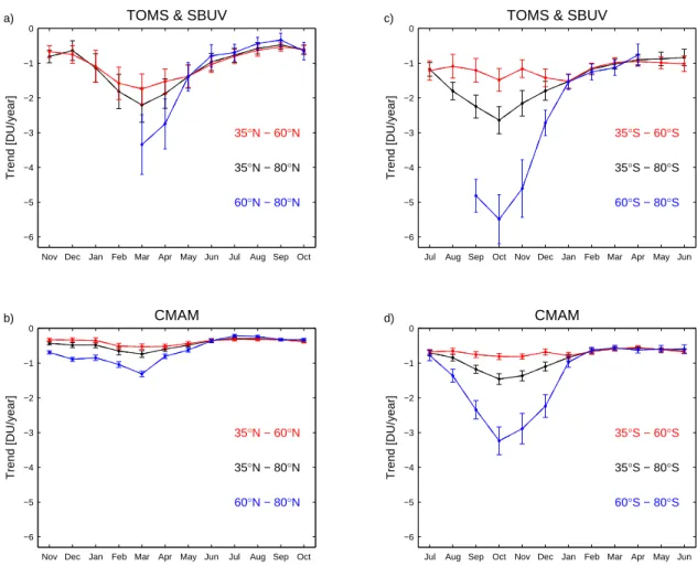
The long-term change in total ozone from observations and from the 45-year transient CMAM run associated with the EESC loading is shown in Fig. 8. The trend coefficients can be expressed in terms of the linear trend during the 1980s (see Sect. 2) and are estimated separately for each month of the year. The magnitude of the trends are weaker in CMAM than in the observations, especially in the northern hemi-sphere. This is not unusual for CCMs (Eyring et al., 2006). Overall the trend functions of ozone show similar charac-teristics in the observations and CMAM. The seasonal cy-cle of the ozone trends have a maximum in spring which is especially strong in the polar regions, reflecting the po-lar springtime ozone depletion. The popo-lar springtime ozone
trends are clearly stronger in the SH. In both hemispheres the polar trends amplify the seasonal cycle of the ozone trends for the entire extratropical region compared to the midlati-tudes. However the summertime trends are nearly identical over middle and polar latitudes.
F&S 2003 demonstrated that in the NH midlatitudes the observed long-term trends are determined by the trends in the winter/spring buildup. There is no need to invoke summer-time ozone chemistry or springsummer-time polar ozone depletion to explain the summertime ozone trends in the NH. In contrast the seasonality of observed trends in the southern midlati-tudes cannot be explained by the springtime trends there. As noted in F&S 2005 the mechanism works better in the SH if the entire extratropical region (35◦S–80◦S) is considered,
implying that springtime polar ozone depletion and transport contribute to the summer ozone trend over SH midlatitudes.
We now examine if the trend function of total ozone from CMAM from summer through to early autumn can be
490 S. Tegtmeier and T. G. Shepherd: Ozone anomalies in CMAM 0.94 0.88 0.81 0.77 0.73 0.61 0.45 0.26 0.96 0.84 0.77 0.71 0.62 0.45 0.34 -0.3 0.93 0.86 0.76 0.67 0.43 0.32 -0.2 -0.1 0.96 0.83 0.70 0.45 0.23 -0.3 -0.1 0.03 0.93 0.76 0.50 0.18 -0.3 -0.1 0.01 -0.1 0.80 0.57 0.23 -0.2 -0.1 0.0 -0.1 -0.1 0.75 0.58 0.09 -0.1 0.17 0.12 0.08 -0.1 1 2 3 4 5 6 7 8 Lag [months] 1 2 3 4 5 6 7 8 CMAM (strong diffusion) 0.80 0.72 0.66 0.59 0.59 0.51 0.42 0.21 0.92 0.81 0.73 0.73 0.66 0.57 0.37 0.34 0.92 0.87 0.85 0.73 0.61 0.41 0.30 0.27 0.95 0.92 0.84 0.70 0.41 0.19 0.29 -0.1 0.94 0.83 0.73 0.45 0.19 0.26 -0.1 -0.2 0.91 0.77 0.46 0.27 0.21 -0.1 -0.2 -0.1 0.82 0.55 0.38 0.29 -0.1 -0.2 -0.1 -0.1 1 2 3 4 5 6 7 8 Lag [months] Mar Apr May Jun Jul Aug Sep 35˚N - 80˚N 0.87 0.79 0.66 0.49 0.34 0.14 0.10 0.30 0.89 0.68 0.52 0.34 0.12 0.23 0.39 0.14 0.84 0.67 0.42 0.26 0.36 0.31 0.05 0.00 0.73 0.50 0.30 0.36 0.39 0.06 0.02 0.18 0.84 0.67 0.59 0.49 0.05 -0.2 -0.1 0.09 0.86 0.69 0.49 0.09 -0.2 -0.1 -0.15 0.17 0.86 0.54 0.25 -0.1 -0.1 0.21 0.15 -0.1
a) TOMS & SBUV b) CMAM
c) Mar Apr May Jun Jul Aug Sep Mar Apr May Jun Jul Aug Sep 1.0 0.9 0.75 0.6 0.3 -0.3 1.0 0.9 0.75 0.6 0.4 -0.4
TOMS & SBUV CMAM (strong diffusion)
CMAM
Fig. 6. Correlation coefficients between ozone anomalies at a given month of the year with ozone anomalies at subsequent months for
35◦N–80◦N, for the observations, the transient CMAM run, and a CMAM time slice run with strong vertical diffusion. Values shaded gray are not statistically significant at the 95% level.
Mar Apr May Jun Jul Aug Sep Oct
0 0.2 0.4 0.6 0.8 1 1.2 1.4
TOMS & SBUV
CMAM
CMAM (strong diffusion)
35°N − 80°N
month
regression coefficient
Fig. 7. Linear regression coefficients between 35◦N–80◦N ozone
anomalies in April and in other months of the year for observations (black) the transient CMAM run (red), and a CMAM time slice run with strong vertical diffusion (blue). The error bars indicate the 1σ uncertainty.
explained by the springtime trends. Therefore we estimate the trend for each month by multiplying the trend value for a
specific selected springtime month with the regression coef-ficient between the two months. Figures 9c and d show the results for the SH midlatitude and extratropical regions based on the trend values for October, November or December. The actual trend function is also displayed. In the southern mid-latitudes the actual trend in summer is significantly stronger than the estimated trends. If, however, the entire extratrop-ical region is considered then the estimates of summertime trends from springtime trends work much better and show the same seasonality as the actual trend function. These re-sults are consistent with the observations.
In the same way, the long-term trends are in line with interannual variability over the entire northern extratropics. This is illustrated by Fig. 9b, which shows the actual trend function from late spring through early autumn together with the estimates of the trend based on the actual trend values for March, April, or May and the regression coefficients for the interannual anomalies. However there are differences between CMAM and the observations for northern midlat-itudes. In the observations, F&S 2003 showed that inter-annual anomalies in NH midlatitudes persist through sum-mer, despite the mixing in of polar air following the vortex breakdown. This is because in terms of total ozone mass,
Nov Dec Jan Feb Mar Apr May Jun Jul Aug Sep Oct −6 −5 −4 −3 −2 −1 0
TOMS & SBUV
Trend [DU/year]
35°N − 60°N 35°N − 80°N 60°N − 80°N a)
Jul Aug Sep Oct Nov Dec Jan Feb Mar Apr May Jun −6 −5 −4 −3 −2 −1 0
TOMS & SBUV
Trend [DU/year]
35°S − 60°S 35°S − 80°S 60°S − 80°S c)
Nov Dec Jan Feb Mar Apr May Jun Jul Aug Sep Oct −6 −5 −4 −3 −2 −1 0 CMAM Trend [DU/year] 35°N − 60°N 35°N − 80°N 60°N − 80°N b)
Jul Aug Sep Oct Nov Dec Jan Feb Mar Apr May Jun −6 −5 −4 −3 −2 −1 0 CMAM Trend [DU/year] 35°S − 60°S 35°S − 80°S 60°S − 80°S d)
Fig. 8. Total ozone trends for midlatitudes (35◦–60◦, red), polar latitudes (60◦–80◦, blue), and the entire extratropical region (35◦–80◦, black) for the northern (left) and southern (right) hemispheres. The observed total ozone trends are shown in the two top panels and the ozone trends for the 45-year transient CMAM run are shown in the two bottom panels. The trends are based on a fit to EESC and are expressed in terms of DU/year during the 1980s (see text for details). The error bars indicate the 1σ uncertainty.
the midlatitude anomalies dominate over the polar anoma-lies; the anomalies seen in Fig. 5 are multiplied by the area of the region. However in CMAM the midlatitude anoma-lies decay rapidly after the vortex breakdown (not shown here), because of the much larger impact of the CMAM po-lar anomalies. As in the SH the estimated trends underpre-dict the summertime trends in NH midlatitudes in CMAM (Fig. 9a). This is in contrast to the observations. The im-plication is that in CMAM the relative importance of Arctic ozone loss is greater than in the observations, just as the in-terannual Arctic anomalies in CMAM have an unrealistically large relative impact on the overall extratropical anomalies (Fig. 5).
5 Summary
The persistence and photochemical decay of springtime total ozone anomalies in CMAM integrated over 35◦–80◦latitude
in both hemispheres is very realistic. The behaviour in the
SH is similar for simulations with and without heterogeneous chemistry, i.e. with or without an ozone hole. The behaviour in the NH is realistic despite unrealistically low ozone vari-ability, but is unrealistic for a simulation with very strong vertical diffusion. This shows that the diagnostic from F&S 2003 does not depend on how the springtime anomalies are created or on their magnitude, but reflects the transport and photochemical decay in the model – as one would expect.
For the entire extratropical region the seasonality of the long-term ozone trends in CMAM for summer through early autumn can be explained by the persistence of the interannual springtime anomalies, as in the observations. This implies that summertime ozone trends are a result of the springtime trends, without the need to invoke changes in summertime chemistry. By considering the entire extratropical region, transport of ozone-depleted air from the polar into the mid-latitude regions following the breakdown of the polar vortex does not affect the relation between springtime and summer-time ozone anomalies and long-term trends. However this
492 S. Tegtmeier and T. G. Shepherd: Ozone anomalies in CMAM
Mar Apr May Jun Jul Aug Sep Oct −1 −0.8 −0.6 −0.4 −0.2 0 0.2 Trend [DU/year] 35°N − 60°N
Trend March April May a)
Sep Oct Nov Dec Jan Feb Mar Apr −1 −0.8 −0.6 −0.4 −0.2 0 0.2 Trend [DU/year] 35°S − 60°S
Trend October November December c)
Mar Apr May Jun Jul Aug Sep Oct −1 −0.8 −0.6 −0.4 −0.2 0 0.2 Trend [DU/year] 35°N − 80°N
Trend March April May b)
Sep Oct Nov Dec Jan Feb Mar Apr −1.6 −1.4 −1.2 −1 −0.8 −0.6 −0.4 Trend [DU/year] 35°S − 80°S Trend October November December d)
Fig. 9. Total ozone trends for the 45-year transient CMAM run (black) and as estimated from the springtime trends (from March, April,
or May in the northern hemisphere, and from October, November, or December in the southern hemisphere) together with the regression coefficients estimated from the detrended data. The trends are shown for midlatitudes (35◦–60◦, top), and the entire extratropical region
(35◦–80◦, bottom) for the northern (left) and southern (right) hemispheres. The trends are based on a fit to EESC and are expressed in terms
of DU/year during the 1980s (see text for details).
is not true for the midlatitudes alone if polar ozone vari-ations are sufficiently large compared to midlatitude varia-tions. This is true in the southern hemisphere for both ob-servations and CMAM, where the ozone hole contributes to midlatitude summertime trends, elevating them above what would be expected based on midlatitude springtime trends and leading to a relatively weak seasonality of the midlat-itude trends. For CMAM this is also true in the northern hemisphere – and in contrast to the observations – because of the relatively large impact, compared to observations, of the CMAM polar anomalies. This results from an unrealistically small midlatitude ozone variability rather than an unrealisti-cally large polar variability.
Acknowledgements. This work was initiated during an earlier
visit by S. Tegtmeier to the University of Toronto and has been supported by funding from the Natural Sciences and Engineering Research Council of Canada, the Canadian Foundation for Climate and Atmospheric Sciences, the Canadian Space Agency, and Environment Canada. The authors are indebted to S. Beagley,
A. Jonsson, and J. de Grandpr´e for assistance with the CMAM data, to V. Fioletov for helpful discussion, and to R. Stolarski and S. Frith from NASA for making the merged satellite data set available. Work at AWI was supported by the EC under contract 505390-GOCE-CT-2004 (SCOUT-O3).
Edited by: M. Dameris
References
Austin, J., Shindell, D., Beagley, S. R., Br¨uhl, C., Dameris, M., Manzini, E., Nagashima, T., Newman, P., Pawson, S., Pitari, G., Rozanov, E., Schnadt, C. and Shepherd, T. G.: Uncertainties and assessments of chemistry-climate models of the stratosphere, At-mos. Chem. Phys., 3, 1–27, 2003,
http://www.atmos-chem-phys.net/3/1/2003/.
Beagley, S. R., de Grandpr´e, J., Koshyk, J. N., McFarlane, N. A., and Shepherd, T. G.: Radiative-dynamical climatology of the
first-generation Canadian Middle Atmosphere Model, Atmos.-Ocean, 35, 293–331, 1997.
de Grandpr´e, J., Beagley, S. R., Fomichev, V. I., Griffioen, E., Mc-Connell, J. C., Medvedev, A. S., and Shepherd, T. G.: Ozone climatology using interactive chemistry: Results from the Cana-dian Middle Atmosphere Model, J. Geophys. Res., 105, 26 475– 26 491, 2000.
Eyring, V., Butchart, N., Waugh, D. W., Akiyoshi, H., Austin, J., Bekki, S., Bodeker, G. E., Boville, B. A., Brhl, C., Chipper-field, M. P., Cordero, E., Dameris, M., Deushi, M., Fioletov, V. E., Frith, S. M., Garcia, R. R. Gettelman, A., Giorgetta, M. A., Grewe, V., Jourdain, L., Kinnison, D. E., Mancini, E., Manzini, E., Marchand, M., Marsh, D. R., Nagashima, T., Newman, P. A., Nielsen, J. E., Pawson, S., Pitari, G., Plummer, D. A., Rozanov, E., Schraner, M., Shepherd, T. G., Shibata, K., Stolarski, R. S., Struthers, H., Tian, W., and Yoshiki, M.: Assessment of tem-perature, trace species and ozone in chemistry-climate model simulations of the recent past, J. Geophys. Res., 111, D22308, doi:10.1029/2006JD007327, 2006.
Fioletov, V. E., Bodeker, G. E., Miller, A. J., McPeters, R. D. and Stolarski, R.: Global and zonal total ozone variations estimated from ground-based and satellite measurements: 1964–2000, J. Geophys. Res., 107, 4647, doi:10.1029/2001JD001350, 2002.
Fioletov, V. E. and Shepherd, T. G.: Seasonal persistence of mid-latitude total ozone anomalies, Geophys. Res. Lett., 30, 1417, doi:10.1029/2002GL016739, 2003.
Fioletov, V. E. and Shepherd, T. G.: Summertime total ozone vari-ations over middle and polar latitudes, Geophys. Res. Lett., 32, L04807, doi: 10.1029/2004GL022080, 2005.
Frith, S., Stolarski, R., and Bhartia, P. K.: Implications of version 8 TOMS and SBUV data for long-term trend analysis, Proceedings of the Quadrennial Ozone Symposium-2004, edited by: Zerefos, C., 65–66, 2004.
Weber, M., Dhomse, S., Wittrock, F., Richter, A., Sinnhuber, B. M. and Burrows, J. P.: Dynamical control of NH and SH win-ter/spring total ozone from GOME observations in 1995-2002, Geophys. Res. Lett., 30, 1583, doi:10.1029/2002GL016799, 2003.
WMO: Scientific Assessment of Ozone Depletion: 1998, World Meteorological Organisation Global Ozone Research and Moni-toring Project Report No. 44, Geneva, 1999.
WMO: Scientific Assessment of Ozone Depletion: 2002, World Meteorological Organisation Global Ozone Research and Moni-toring Project Report No. 47, Geneva, 2003.