Econometric models of eleven single family housing markets

ECONOMETRIC MODELS OF ELEVEN SINGLE FAMILY HOUSING MARKETS by

IRENE D. JENKINS B.A., History

Brandeis University, Waltham, MA (1968)

M.A., History

Harvard University, Cambridge, MA (1973)

and

MARY HELEN SCHAEFFER B.S., Business Administration

University of San Francisco, San Francisco, CA (1978)

Submitted to the Department of Urban Studies and Planning and the Department of Architecture in Partial Fulfillment of the Requirements of the Degree of Master of Science

in Real Estate Development

at the Massachusetts Institute of Technology September 1989

@ Irene D. Jenkins and Mary Helen Schaeffer 1989

The authors hereby grant to MIT permission to reproduce and to distribute copies of this thesis document in whole or in part.

Signature of Author___

Irene D. Jenkins Department"6f Urban Studies and Planning July 31, 1989 Signature of Author r H ce Department of Architecture July 31, 1989 Certified by__ William C. Wheaton Associate Professor, Economics Thesis Supervisor

Accepted by

Michael Wheeler Chairman, Interdepartmental Degree Program in Real Estate Development

R(

tCEj

ECONOMETRIC MODELS OF ELEVEN SINGLE FAMILY HOUSING MARKETS by

IRENE D. JENKINS and MARY HELEN SCHAEFFER

Submitted to the Department of Urban Studies and Planning and the Department of Architecture on July 31, 1989

in Partial Fulfillment of the Requirements of the Degree of

Master of Science in Real Estate Development ABSTRACT

Using data from 1960 through 1988 on prices, building

permits, level of economic activity, and demographic

characteristics in 14 metropolitan areas, we developed and estimated econometric models for the single family housing market. The areas studied were: New York, Chicago, Detroit, Denver, Houston, San Francisco, Minneapolis, Philadelphia,

Cleveland, Los Angeles, Dallas, Atlanta, Boston, and

Baltimore. We used the models to make an eleven year

(1989-1999) forecast of real housing prices and building

permits in eleven of the fourteen metropolitan areas. We were unable to obtain reasonable estimation results for Chicago, Detroit, and New York and so did not make forecasts

for these three cities.

Based upon our forecasts, real prices will rise over the next decade, with or without recession, in Dallas, Houston, Denver, Cleveland, San Francisco, Boston, Los Angeles, Philadelphia, and Baltimore. Real prices will decline in Minneapolis and Atlanta. The level of construction will rise in Dallas, Houston, Cleveland, Boston, Philadelphia, Baltimore, Minneapolis, and Atlanta and will decline in Denver. In San Francisco and Los Angeles, construction will remain near 1987/1988 levels.

Thesis Supervisor: William C. Wheaton

Table of Contents Abstract . . . . . . . . . 2 Table of Contents . . . . 3 List of Figures. . . . . . - 4 List of Tables . .. . . . 5 Chapter 1: Introduction . . . . 6

Chapter 2: The Data . . . - - 10

Chapter 3: The Models and The Estimation Results . . .26

Chapter 4: The Forecasts . . . .37

Chapter 5: Conclusions . . . 78

References . . . . . - - - - 80

Appendix A: Metropolitan Area Definitions . . . 85

List of Figures

Figure 2.1: Relative Changes in Real Prices . . . . .25

Figure 4.1-11: Forecasts of Prices and Permits 4.1: Denver . . . . 42 4.2: Houston. . . . . . . . . . 45 4.3: San Francisco. . . . 48 4.4: Minneapolis . . . . 51 4.5: Philadelphia . . . . 54 4.6: Cleveland . . . 57 4.7: Los Angeles . . . . 60 4.8: Dallas . . . . 63 4.9: Atlanta. . . . . 66 4.10: Boston. . . . . 69 4.11: Baltimore. . . . 72

List of Tables

Table 2.1: Equations Used to Create New Variables . . .21 Table 2.2: Differences in Prices Between Cities . . . 22

Table 2.3: Percentage Change in Real Prices

1963 vs. 1988 . . . . 23

Table 2.4: Most Expensive to Least Expensive Cities . . 24 Table 3.1: Price Equations . . . 34 Table 3.2: Permit Equations. . . . 35

Table 3.3: Speed of Price Adjustment . . . 36

Table 4.1: Growth Factors and Other Assumptions . . . 73 Table 4.2a: Forecasts of Prices and Permits by City

(No Recession). . . . .74 Table 4.2b: Forecasts of Prices and Permits by City

CHAPTER ONE INTRODUCTION

Our objective was to study local markets for single family housing and to create econometric models for each market to forecast supply, demand, and real housing prices

for the next ten years.

Our choice of cities was influenced by the availability of adequate time series data. The cities we studied were: Denver, Houston, Chicago, San Francisco, Minneapolis/St.

Paul, Philadelphia, Cleveland, Los Angeles, Dallas, Detroit, Atlanta, New York, Boston, and Baltimore. For this study, a

"city" is generally equivalent to the MSA or PMSA, or a combination of PMSA's. Descriptions of the data and its sources and limitations are discussed in detail in Chapter Two.

Other authors have proposed models for the single family housing market. Most of these studies have focussed on

housing at the national level; very little work has been done with local housing markets. We have attempted to determine which of these models, if any, best fit the data we have on employment, population, real personal income, building

permits, rents, mortgage rates, average sales prices, and inflation.

single family housing and supply of new single family housing units. Are prices determined by lower mortgage rates,

anticipated appreciation, relative costs of buying versus renting, a combination of these factors, or something else? IS the level of construction determined by economic growth or decline, changes in incomes, house prices, and/or mortgage rates, or the level of construction last year?

In some of the cities, growth controls restrict the creation of new housing; in others, development is almost entirely uncontrolled. How do these differences affect the performance of the market?

The models and the estimation results for the supply and price equations are presented in Chapter Three. The

variables affecting supply and demand were different from market to market.

Having estimated the equations for construction and real prices, we created a stock flow model to forecast (using a recession and nonrecession scenario) permits, stock, and prices utilizing forecasts of changes in employment, population, and income as well as mortgage rates and

inflation.

We were unable to obtain reasonable estimation results for Chicago, Detroit, and New York and did not make any

forecasts for these three cities. Based upon our forecasts, real prices will continue to rise over the next eleven years,

recession or not, in San Francisco, Boston, Los Angeles, Philadelphia, and Baltimore. Although real prices have increased sharply since 1983 in Minneapolis and Atlanta, we project a decline in real prices in these two cities between now and 1999. The "oil patch" cities of Dallas, Houston, and

Denver will reverse their recent trend of price decline and prices will slowly rise again. Cleveland will experience a year or two of declining prices and then rising prices in the early 1990's.

The level of construction will reverse its recent decline and will rise in Dallas, Boston, Philadelphia,

Baltimore, Minneapolis, and Atlanta. Construction will also rise, though not as rapidly, in Cleveland and Houston,

although it will level off in Houston in the mid 1990's. In Los Angeles and San Francisco, new construction will not change much from 1987/1988 levels. In Denver, construction, which has just begun to show an increase after several years of decline, will decrease again and then level off.

We hope to put each locality in perspective and

highlight some of the striking differences between them in terms of prosperity, decline, and housing prices and supply. The methodology, forecasts, and a market summary for each city are presented in Chapter Four.

In Chapter Five, we draw some conclusions about the operation of these markets and the factors that affect

housing prices and construction. We also make some

observations about the utility and limitations of this type of model.

CHAPTER TWO

THE DATA

We collected data for 25 metropolitan areas. Because complete data for 11 of the cities were unavailable, we were able to study only 14 of the 25 metropolitan areas. Our

dataset reflects recessions that occurred in 1970-1971, 1974-1975, and 1981-1982, the entry of the "baby boomers" into the housing market, decreasing family size, a period of double digit inflation, and increased female labor force participation.

Our database included figures for each area, from 1960 through 1988, on non-agricultural employment (EMP),

population (POP), total real personal income (YPI), numbers of single family (SFPRMT) and multi-family permits (MFPRMT) issued, average Federal Home Loan Bank Board mortgage rates

(MTGR), average resale single family home prices (SFPRICE) (from 1963 to 1988 only), and national inflation rates (INF).

The data on employment, population, personal income, single and multi-family permits, and inflation came from the U.S. Department of Commerce. The Federal Home Loan Bank Board provided contract mortgage rates and purchase prices

AREA DEFINITIONS

The metropolitan area definitions are generally

consistent with census bureau definitions of either MSAs or PMSAs or aggregations of them. The San Francisco

metropolitan area includes Oakland and the Boston metropolitan area includes Suffolk, Middlesex, Essex, Norfolk, and Plymouth counties. (See Appendix A,

Metropolitan Area Definitions.) Because the Census Bureau changed its metropolitan area definitions over the time

series, obtaining permit data for the same area from year to year presented some difficulties, which we overcame by using tables that listed individual permit issuing places, e.g. municipalities, rather than the metropolitan area summary tables.

Our study, of necessity, assumed that each metropolitan area constitutes a housing market, which is questionable. For example, New York includes the five counties (boroughs) of New York City, plus Westchester, Rockland, and Putnam

counties, but does not include Nassau and Suffolk counties on Long Island or the New Jersey suburbs of New York. Chicago includes only Cook and Du Page counties. Housing markets may be smaller, larger, or just different from our metropolitan area definitions.

PERMITS

There were some inconsistencies in the dataset. The 1972 permit data from the Construction Reports, C40 series, showed different numbers of permits than the Commerce

Department numbers for that same year. We are not certain why this is the case, since the data came from the same source. The Commerce Department permit numbers for 1972 through 1987 may reflect revised unpublished annual figures or adjustments made for places that issued permits but did not report them to the Census Bureau. We assumed that this data was the most accurate and adjusted the permit data from

1960 to 1972 proportionately for consistency with the Commerce Department data.

The total number of permit-issuing places increased from approximately 10,000 in 1960 to 17,000 in 1988. This may have resulted in an underestimate of supply in the early years of the time series. However, because we are dealing only with metropolitan areas and these areas were

substantially covered by permit-issuing authorities even in 1960, we believe that this is a relatively unimportant

discrepancy. For the years 1960 through 1965, the permit data also includes contract awards for publicly owned units. Since publicly owned housing is mostly multi-family rather than single family, this was a minor inconsistency.

Variation in local definitions of single family structures may have had more effect in some cities. The permit data is based on local building permit officials' reports on numbers of permits issued. There is no way of knowing whether they have consistently defined a structure with one unit. For example, does the local official consider a rowhouse or a one to four unit building a single family or a multi-family unit? We have no way of measuring, correcting, or compensating for these local variations. The Census Bureau's Building Permits Survey defines single family houses to include all detached one-family houses and all attached one-family houses

separated by a wall that extends from ground to roof with no common heating system or interstructural public utilities. The definition excludes mobile homes.

Permit data is a proxy for actual construction of housing, although it has been found to be a reliable

indicator of the level of construction. Census Bureau

surveys indicate that construction is undertaken for all but a small percentage of permit-authorized units. In 1973, the Census Bureau reported that continuing monthly sample surveys for the nation as a whole indicated that only about 2 percent

of permit-authorized housing units are never constructed.1

Only a small percentage of units constructed in

permit-issuing areas are constructed without permits. In 1988 the Census Bureau reported that a study spanning 4 years

showed that about 3 percent of the single family houses built in permit-issuing places are built without a permit.2

Nationally, less than 5 percent of all privately owned housing units built are constructed in areas that do not require building permits.3

Permit data does not distinguish units by form of ownership or tenure. For this study, we assumed that all

single family units in an area are part of the same for-sale market. Our single family data does not include condominiums

in multi-family structures, which, depending upon the place and the time, may also be part of the same "single family" for-sale market. This inability to distinguish rental from for-sale units is probably not as big a problem for a study of sales prices for single family homes as it would be for a

study of the rental market.

STOCK

We obtained 1960, 1970, and 1980 housing stock numbers for each area from the censuses for those years, with the intention of using them as benchmarks and to determine, in conjunction with the permit numbers, the survival rates for single family housing units each area and whether the rate changed from decade to decade. However, the data proved to be impossible to use for those purposes. The stock numbers reported in the 1970 and 1980 censuses were inconsistent,

implying spontaneous generation of new housing units, conversion of multi-family to single family units, or negative depreciation rates. We think that this is

attributable to a change in the reporting definition from number of units in a structure to number of units at an address, which could markedly increase the count of the "single family" stock. Although the 1960 and 1970 figures appeared to be more consistent with permit data, we used a constant annual survival rate of .998 for all areas in our regressions rather than apply a different rate, derived from the census and permit data, to each area. Therefore, our data does not take into account differences in survival rates among areas and probably does not reflect the actual single family stock number after 1960 for any area. We used the 1960 stock number reported in the census as the benchmark for subsequent stock numbers, which we obtained by multiplying the prior year's stock by .998 (the survival rate) and adding the prior year's permits.

ESTK

The variables ESTK (STOCK/EMP) and ESTK1 (STOCKt-1/EMP) represents housing shortfall or surplus in relation to demand

CPI

The CPI is based upon the national inflation rate, with 1960 equal to 1.00.

DEMOGRAPHIC VARIABLES

The WAGE and SIZE variables are approximations, not actual data. The SIZE variable (population/employment) as a measure of household size, assuming one household per

employee, is somewhat problematic, because it more directly measures labor force participation and may indicate changes in such participation rather than changes in household size. WAGE (real personal income/employment), is a proxy for

household income, does not reflect income distribution or disposable income, which may vary from place to place.

COST OF CAPITAL VARIABLES

We tried three variations of a variable, USER, to measure the homebuyer's cost of capital. USER was the

mortgage rate times one minus the tax rate, representing the nominal after-tax cost of capital. USER1 was similar, except that it included the effects of inflation and represented the real after-tax cost of capital. USER2 also included the

percentage change in nominal housing pricest-1 as a way of capturing the effects of both appreciation and inflation in

the after-tax cost of capital.

PRICES

Real single family prices are nominal prices deflated with the applicable CPI. Single family home price data from the Federal Home Loan Bank Board may not accurately represent average prices in an area because it comes from data on

mortgages that they purchase, not a representative sample of all transactions. This data also does not control for

changes in the characteristics of houses sold over time. Contract mortgage interest rates do not reflect changes or variations in other fees and charges over time or from one

area to another. A complete list of the variables created and their formulas is provided in Table 2.1.

THE REGIONAL MARKETS

We hypothesized that local housing markets behave

differently from one another. The markets in these 14 cities did show some similarities over the 25 years for which we have price data (1963-1988). In the 1980's, sharply rising nominal prices was the trend in all the cities. In addition, all cities experienced a peak and then a decline in nominal prices at some point during 1981-1982, although the size of this spike varies among localities. Because inflation masks the real changes in prices, we used real, inflation-adjusted,

prices in our analysis and comparison of the markets and in our forecasts rather than nominal prices.

Between 1963 and 1988 the relative "real priciness" of the cities changed. Table 2.2 shows the differences in real prices for single family homes across the fourteen cities. For example, in 1963 the real average home price in Denver was $4,900 less than the real average home price in Houston,

but in 1988 the real average home price in Denver was $5,800 more than in Houston. A more extreme example is a comparison of Cleveland and Los Angeles. In 1963 real prices in

Cleveland averaged $1,400 less than in Los Angeles, but by

1988 real prices in Cleveland averaged $23,000 less. In 1963

a move from the least expensive city (Philadelphia) to the most expensive city (New York) entailed a higher average real price of $9,700. In 1988 a move from the least expensive city (Cleveland) to the most expensive (San Francisco)

entailed an average real price differential of $26,900. The percentage changes in real prices from 1963 to 1988 are shown

in Table 2.3. Clearly, some areas, most notably Cleveland, Houston, Detroit, and Chicago, did not profit nearly as much

as others from the "real estate boom" of the 1980's. What caused the widening difference in housing prices from city to city since 1963? Was it a by-product of the decline in

midwestern industry or a change in housing policy or something else, such as population shift?

In 1963 the six most expensive areas (in decreasing order) were: New York, San Francisco, Houston, Los Angeles, Chicago, and Boston. (See Table 2.4-Most Expensive to Least Expensive Cities.) By 1988 the list had changed to: San

Francisco, Boston, New York, Los Angeles, Baltimore, and Philadelphia. The coastal cities continued to be the most expensive places to live, but in 1988 the list did not include any "heartland" cities. Chicago and Houston were replaced by Baltimore and Philadelphia, two near-coastal cities.

The level of construction (permits) was quite different from one area to another. However, there were similarities. In most of our cities, permits reached a trough in 1970, in 1974 or 1975, and in 1981 or 1982. These were recession years. The peaks were less consistent. In most areas permits either reached a peak or were still rising in 1986 except in the "oil patch" cities of Houston, Dallas, and Denver.

In most of our cities the level of permits in 1988 was at or below the level in 1960. The exceptions were

NOTES TO CHAPTER TWO

1_{Construction Reports, C40-72-13, Appendix I.} 2

BUILDING PERMITS SURVEY DOCUMENTATION: Metropolitan, Consolidated Metropolitan and Primary Metropolitan Statistical Area Statistics for Permit Authorized Construction, 1988.

TABLE 2.1

EQUATIONS USED TO CREATE NEW VARIABLES: WAGEt YPIt/EMPt

SIZEt (HOUSEHOLD SIZE) _{= POPt/EMPt}

DEMPt (CHANGE IN EMPLOYMENT) _{= EMPt - EMPt-1}

ESTKt _{= STOCKt/EMPt}

ESTK1t _{= STOCK t-1/EMPt}

DPOPt (CHANGE IN POPULATION) _{= POP t - POP t-1}

DYPIt (CHANGE IN REAL PERSONAL INCOME) ₌ YPIt - YPIt-1

CPIt(1960=1) = CPIt-1 * (1 + INFt * .01)

RPRICEt (REAL PRICE) = _{(NOMINAL PRICEt * CPI t=}

1 9 6 3)/CPIt

DRPRICEt(CHANGE IN REAL PRICE) = (RPRICEt-RPRICEt-1)/RPRICEt-1 USERt (USER COST OF CAPITAL) = MTGRt * .6

USERlt (USER COST OF CAPITAL 1) =

for years 1960-1986 _{= MTGRt * .6}

- INFt

for years 1987 and later = MTGRt * .72 - INFt

USER2 (USER COST OF CAPITAL 2) =

for years 1960-1986 = MTGRt * .6 - DRPRICE * 100 - INFt

for years 1987 and later = MTGRt * .72 - DlP1ICEt-l*100 _{- INFt}

STOCKt = STOCKt-1 _{* DEPt + PERMITSt-1}

ERPRICEt _{= EMPt * RPRICE}

t-1 EUSER _{= EMP *} USERt EUSERlt _{= EMPt *} USERlt EUSER2 _{= EMP *} USER2t

VARIABLES IN THE DATASET: EMPLOYMENT, POPULATION, REAL PERSONAL INCOME, MULTI-FAMILY PERMITS, RENT INDEX, MORTGAGE RATE, NOMINAL PRICES, SINGLE FAMILY PERMITS, INFLATION RATE.

TABLE 2.2

DIFFERENCES IN REAL PRICES BETWEEN CITIES

1963 REAL PRICE (IN 000'S)

CHICAGO -2.9 2.7 6.5 1.1 -0.3 3.4 2.4 2.7 -3.1 0.9 4.9 SAN FRANCISCO 5.7 MINNEAPOLIS 9.5 3.8 PHILADELPHIA 4.1 -1.6 -5.4 CLEVELAND 2.7 -3.0 -6.8 -1.4 LOS ANGELES 6.4 0.7 -3.1 2.3 3.7 DALLAS 5.3 -0.4 -4.2 1.2 2.6 -1.1 5.6 -0.1 -3.9 1.5 2.9 -0.8 -0.2 -5.9 -9.7 -4.3 -2.9 -6.6 3.8 -1.8 -5.6 -0.3 1.2 -2.6 7.9 2.2 -1.6 3.8 5.2 1.5 DETROIT 0.3 ATLANTA -5.5 -5.8 NEW YORK -1.5 -1.8 4.0 BOSTON 2.6 2.3 8.1 4.0 BALTIMORE

1988 REAL PRICE (IN 000'S)

HOUSTON -3.2 CHICAGO -23.6 -20.3 SAN FRANCISCO -7.2 -4.0 16.3 MINNEAPOLIS -8.2 -5.0 15.4 -1.0 PHILADELPHIA 3.3 6.6 26.9 10.6 11.5 CLEVELAND -20.0 -16.8. 3.6 -12.8 -11.8 -23.3 LOS ANGELES -3.2 0.0 20.3 4.0 5.0 -6.6 16.8 DALLAS 2.7 5.9 26.2 9.9 10.9 -0.6 22.7 5.9 -8.1 -4.9 15.4 -0.9 0.1 -11.4 11.9 -4.9 -21.4 -18.2 2.1 -14.2 -13.2 -24.7 -1.4 -18.2 -22.2 -18.9 1.4 -14.9 -14.0 -25.5 -2.2 -18.9 -8.4 -5.2 15.2 -1.2 -0.2 -11.7 11.6 -5.2 DETROIT -10.8 ATLANTA -24.1 -13.3 NEW YORK -24.8 -14.0 -0.7 BOSTON -11.1 -0.3 13.0 13.8 BALTIMORE DENVER -4.9 -3.3 -6.3 -0.6 3.2 -2.2 -3.6 0.1 -1.0 -0.7 -6.5 -2.4 1.6 HOUSTON 1.6 -1.4 4.3 8.1 2.7 1.3 5.0 3.9 4.2 -1.6 2.4 6.5 DENVER 5.8 2.5 -17.8 -1.5 -2.4 9.1 -14.2 2.5 8.4 -2.4 -15.6 -16.4 -2.6

TABLE 2.3

PERCENTAGE CHANGE IN REAL AND NOMINAL PRICES

1963 1988 1963 1988

REAL REAL PERCENT NOMINAL NOMINAL PERCENT PRICE PRICE CHANGE PRICE PRICE CHANGE

DENVER 20.3 34.1 68% 20.3 132.2 551% HOUSTON 25.2 28.4 13% 25.2 109.9 336% CHICAGO 23.6 31.6 34% 23.6 122.4 418% SAN FRANCISCO 26.6 51.9 95% 26.6 201.1 657% MINNEAPOLIS 20.9 35.6 70% 20.9 137.9 560% PHILADELPHIA 17.1 36.6 114% 17.1 141.6 729% CLEVELAND 22.5 25.0 11% 22.5 97.0 331% LOS ANGELES 23.9 48.4 102% 23.9 187.3 683% DALLAS 20.2 31.6 57% 20.2 122.4 507% DETROIT 21.3 25.7 21% 21.3 99.5 368% ATLANTA 21.0 36.5 74% 21.0 141.3 574% NEW YORK 26.8 49.8 86% 26.8 192.8 620% BOSTON 22.7 50.5 122% 22.7 195.7 761% BALTIMORE 18.7 36.8 97% 18.7 142.4 661%

TABLE 2.4

MOST EXPENSIVE TO LEAST EXPENSIVE CITIES

NEW YORK SAN FRANCISCO HOUSTON LOS ANGELES CHICAGO BOSTON CLEVELAND DETROIT ATLANTA MINNEAPOLIS DENVER DALLAS BALTIMORE PHILADELPHIA RANK RANK 1963 1988 1 3 2 1 3 11 4 4 5 10 6 2 7 13 8 12 9 7 10 8 11 9 12 10 13 5 14 6

FIGURE 2.1

REAL PRICES FOR HOMES 1963 VS. 1988

-/

k I7 kNk

DEN HOU CHI SAF MIN PHI CLE LOS DAL DET ATL NEW BOS BAL

CITY 1988 50 40 30 20 10 1963

CHAPTER THREE

THE MODELS AND THE ESTIMATION RESULTS

Although the significance and magnitude of the effect of the variables is different for each of the cities, the

underlying structure of each model is similar. Our models consisted of equations for real housing price and level of new construction (as evidenced by building permits) which we estimated using the 1960 through 1988 dataset. (See Tables

3.1 and 3.2: Price and Permit Equations.) Our stock equation was:

STOCKt = STOCKt-₁(1-depreciation rate) ₊ PERMITSt-1

We wanted to create dynamic models for each city where demand is not necessarily equal to supply at any given time, and where prices depend in part upon the amount of new

housing built as well as demographic and cost of capital variables. Given the lead time needed to bring new housing stock to market, it seemed reasonable to assume that the market does not clear completely during each period, but rather is continually moving toward its long-run equilibrium price level.

PRICE EQUATIONS

Our first effort at establishing equations for prices was to run regressions of various combinations of demographic

(demand), affordability (cost of capital), and housing stock (supply) variables to see which variables were significant in which cities, using our firsthand real estate experience and our personal knowledge of the Boston, Baltimore, Cleveland,

San Francisco, Los Angeles, Detroit, and New York markets to select the initial combinations. We approached the price equations in this manner because there has not been

definitive work done on prices and permits at the local level and our purpose was to construct a model that would

accurately reflect the behavior of local markets. Our "map" for attempting to describe this local behavior was However, the results were not particularly good, with R 2's in the

.70-.85 range, unexpected signs of the coefficients, and

insignificant t-statistics for variables that we had expected to be significant in explaining price fluctuations.

We then turned to theory for assistance, estimating equations of the form:

PRICE - RICEt-1 a(PRICE*-PRICEt-1 [equation 1] which can be expressed as

PRICEt = aPRICE + (1-a)PRICEt-₁

where PRICE is the long-run equilibrium price level, and

[equation 2]

which we can solve for PRICE *

PRICE = b/c + d/cWAGE + e/cUSER + f/cSIZE

-1/cSTOCK/EMP [equation 3].

By substituting PRICE in equation 3 for PRICE in equation 1 we obtain an equation that we can estimate for PRICEt'

PRICEt = ab/c + ad/cWAGE + ae/cUSER + af/cSIZE -a/cSTOCK/EMP + (1-a)PRICEt-₁ [equation 4].

The variables ESTK (STOCK/EMP) and USER were problematic in that it was difficult to find combinations of them and other variables such that their coefficients had the expected negative sign. As a result, some of the equations that we

selected to use in our models had relatively low R 's (one as low as .59) and included variables whose t-statistics did not indicate significance. (See Table 3.1: Price Equations.)

In three cities--New York, Chicago, and Detroit--we

abandoned the effort to develop reasonable price equations as a result of inadequate results and time constraints.

Therefore, we were unable to forecast prices and permits for those three cities. In New York, the exclusion of Nassau and

Suffolk counties as well as the New Jersey suburbs of New York City from the data created a problematic market

definition. In Chicago, the coverage of the data (see Chapter Two) may also have affected the results. We began with partial data on 25 cities, were able to complete the

dataset for 14 of those, and were able to find reasonable price equations for forecasting for only eleven cities.

In all cases, except Atlanta, our final equations

included the variable ESTK. In Atlanta, ESTK1 yielded better results.

Seven of the final equations--for Denver, Houston, San Francisco, Minneapolis, Cleveland, Dallas, and Atlanta--used

USER2. In Boston and Philadelphia, MTGR, the nominal

mortgage rate, yielded a higher R2 than USER2 and was used instead. In Los Angeles and Baltimore, USER yielded the best results.

We used RPRICEt-1 in all of the final equations. The coefficients of RPRICEt-1 in these equations varied

substantially. Since 1 minus the coefficient of RPRICEt-1 represents the percentage price adjustment in one year (the speed of adjustment) we can see that the Dallas and Houston markets clear more quickly than the others and that the San Francisco and Atlanta markets clear more slowly. (See Table 3.3, Speed of Price Adjustment.)

In Philadelphia and Baltimore the coefficients of

RPRICEt-1 were greater than one, resulting in negative speeds of adjustment. These results are logically inconsistent,

implying that more than 100 percent of this year's price is accounted for by last year's price. We used these equations

for our forecast because removing RPRICEt-1 from the

equations yielded even more peculiar forecast results. (See Chapter Four.)

Our equations for only three cities (Denver, San

Francisco, and Baltimore) included either WAGE or WAGEt-l' Although we estimated equations using SIZE in

combination with ESTK and USER, we did not include SIZE in the final equations because better overall results were obtained with the other combinations.

We obtained the best results for price equations in Boston and Los Angeles, with high R2's, Durbin Watsons close to 2.000, and t-statistics indicating significance for all of the variables included in the equations.

PERMIT EQUATIONS

For the supply side of our model, we did our regression analysis using combinations of economic and demographic

indicators (employment, population, income), supply variables (stock and lagged permits), demand variables (e.g. wage, size, mortgage rate), and price level and change in prices. We included a constant in all equations.

The general form of the equation that we estimated and used for our final forecast was:

PERMITt = a+ bPERMITt-1 + cSTOCK + dDRPRICE + eEMP (or

eDEMP) + fPOP + gINCOME + hWAGE + iSIZE + jMTGR (or

All of the final permit equations included STOCK or

PERMITt-1. The equations for Denver and Dallas included both STOCK and PERMITt-1. PERMITt-1 was _{a significant variable in} Houston (t-statistic of 7.479) Cleveland (2.252) and Boston

(2.231) indicating a possible "herd" effect in these cities. Either MTGR or USER2 were included in seven equations and are significant variables in three of these, indicating that, in these markets, builders build more when mortgage rates are down.

Change in real prices (DRPRICE), with t-statistics indicating significance, was included in the equations for only five cities (Baltimore, Boston, Los Angeles,

Philadelphia, and Cleveland) while real price (RPRICE) was not included in any of our equations. Surprisingly, price variables were insignificant or the unexpected sign in six cities. Believing that builders would respond to higher prices by building more, we expected RPRICE, RPRICEt-l' or DRPRICE to be significant and positive in accounting for changes in supply. Our results suggest that, at least in some markets, builders may rationally look ahead and consider that prices may decline if everyone starts building.

Income (YPI) was used only for Boston, population (POP) for Houston and Los Angeles, employment (EMP) for Atlanta and Dallas, and change in employment (DEMP) for Denver,

t-statistics indicating significance, in six cities:

Minneapolis, Cleveland, Dallas, Atlanta, Philadelphia, and Baltimore. (In San Francisco it was included but was not significant.)

SIZE was significant in Atlanta and in Dallas with positive signs and in Minneapolis with a negative sign. As discussed in Chapter Two, the SIZE variable is subject to several interpretations. With a positive sign it could indicate that builders build when household size increases, which may result in a demand for more housing or for housing different fro m what is available. With a negative sign, it

could indicate that builders build as labor force

participation increases. A fall in SIZE, the ratio of

population to employment, may occur when either the number of household members in the labor force or the ratio of total employees to population increases which may increase demand, i.e. either the number of households able to purchase single family housing or the number of people able to form

households or both.

R 2's for our equations ranged from .65 for San Francisco to .92 for Boston. Durbin-Watsons ranged from 1.429 to

2.097. Based upon the t-statistics, the equations for

Atlanta and Boston include only significant variables. Four of the five variables used for Philadelphia, Los Angeles, and

have t-statistics indicating significance. (See Table 3.2, Permit Equations.)

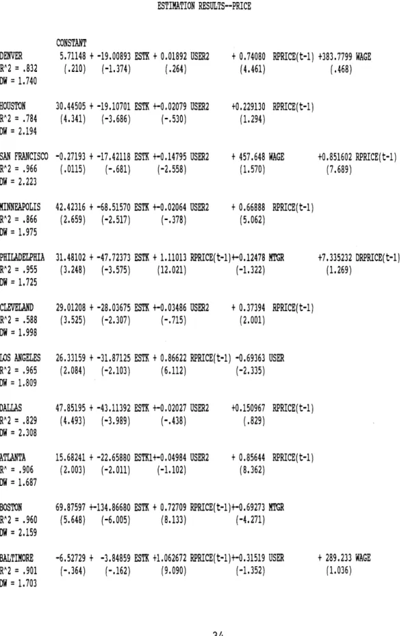
TABLE 3.1 ESTIMATION RESULTS--PRICE CONSTANT 5.71148 + -19.00893 ESTK + 0.01892 USER2 (.210) (-1.374) (.264) 30.44505 + -19.10701 ESTK +-0.02079 USER2 (4.341) (-3.686) (-.530) -0.27193 + -17.42118 ESTK +-0.14795 USER2 (.0115) (-.681) (-2.558) 42.42316 + -68.51570 ESTK +-0.02064 USER2 (2.659) (-2.517) (-.378) + 0.74080 (4.461) +0.229130 (1.294) + 457.648 WAGE (1.570) RPRICE(t-1) +383.7799 WAGE (.468) RPRICE(t-1) +0.851602 RPRICE(t-1) (7.689) + 0.66888 RPRICE(t-1) (5.062) 31.48102 + -47.72373 ESTK + 1.11013 RPRICE(t-1)+-0.12478 MTGR (3.248) (-3.575) (12.021) (-1.322) 29.01208 + -28.03675 ESTK +-0.03486 USER2 (3.525) (-2.307) (-.715) 26.33159 + -31.87125 (2.084) (-2.103) + 0.37394 (2.001) +7.335232 DRPRICE(t-1) (1.269) RPRICE(t-1)

ESTK + 0.86622 RPRICE(t-1) -0.69363 USER (6.112) (-2.335) 47.85195 + -43.11392 ESTK +-0.02027 USER2 (4.493) (-3.989) (-.438) 15.68241 + -22.65880 ESTK1+-0.04984 USER2 (2.003) (-2.011) (-1.102) 69.87597 +-134.86680 (5.648) (-6.005) +0.150967 (.829) + 0.85644 (8.362) RPRICE(t-1) RPRICE(t-1) ESTK + 0.72709 RPRICE(t-1)+-0.69273 MTGR (8.133) (-4.271)

-6.52729 + -3.84859 ESTK +1.062672 RPRICE(t-1)+-0.31519 USER

(-.364) (-.162) (9.090) (-1.352) + 289.233 WAGE (1.036) DENVER R^2 = .832 DW 1.740 HOUSTON R^2 .784 DW 2.194 SAN FRANCISCO R^2 .966 DW 2.223 MINNEAPOLIS R^2 = .866 DW 1.975 PHILADELPHIA R^2 = .955 DW = 1.725 CLEVELAND R^2 .588 DW = 1.998 LOS ANGELES R^2 .965 DW = 1.809 DALLAS RA2 .829 DW 2.308 ATLANTA RA = .906 DW = 1.687 BOSTON RA2 .960 DW = 2.159 BALTIMORE RA2 = .901 DW 1.703

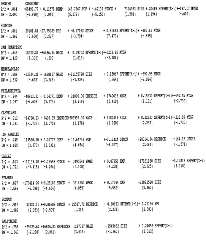
TABLE 3.2 ESTIMATION RESULTS--PERMITS CONSTANT -68498.79 + 0.11571 DEMP (-2.920) (3.040) 20101.81 +27.75089 POP (3.600) (3.527) + 148.7867 POP + -.42139 STOCK + (5.172) + -0.17162 STOCK (-3.794) (-5.153) 7324983 SIZE +.20419 SFPRMT(t-1)+-197.17 MTGR (1.501) (1.194) (-.602) + 0.81683 SFPRMT(t-1)+ -402.61 MTGR (7.479) (-.635) 18520.84 +66486.34 WAGE (1.302) (.200) -13734.21 + 1668117 WAGE (-.698) (3.243) -48913.33 + 0.04371 DEMP (-4.606) (3.273) -14780.23 + 7499.35 DRPR (-1.737) (3.070) 113530.70 + 0.01777 DEMP (3.870) (2.631) -112139.10 +-0.19598 STOCK + (-3.418) (-4.264) -170414.20 +-0.28189 STOCK + (-6.596) (-4.654) 37921.15 +-0.06689 STOCK + (2.953) (-2.505) -29929.62 +16805.83 DRPRICE+ (-2.288) (2.061) + 0.29702 (1.618) +-11155720 SIZE (-3.329) + 21006.06 DRPRICE (2.919) CE+503599.30 WAGE (3.178) + 14.64743 POP (4.454) 3495541 WAGE (5.108) 3314750 WAGE (4.055) 15587.72 DRPRICE j.313) 1287327 WAGE (3.639) SFPRMT(t-1)+-1203.85 MTGR (-2.984) + 0.15067 (.764) SFPRMT(t-1)+ -697.95 MTGR (-2.024) + 1740635 WAGE (5.410) + 1182449 SIZE (1.020) +-0.12424 STOCK (-4.097) + 0.07956 EMP (4.208) + 0.17744 EMP (5.552) + 0.15530 SFPRMT(t-1)+-440.45 MTGR (1.191) (-2.730) + 0.32327 SFPRMT(t-1)+-223.89 MTGR (2.252) (-1.730) SAN FRANCISCO RA2 .645 DW = 1.429 MINNEAPOLIS RA2 = .689 DW = 1.632 PHILADELPHIA R^2 .844 DW = 2.097 CLEVELAND RA2 .912 DW = 1.781 LOS ANGELES R^2 .749 DW = 1.885 +-164.16 USER2 (-1.571) +0.17816 SFPRMT(t-1) (1.110) + 0.30623 SFPRMT(t-1)+ 0.25196 YPI (2.231) (2.003) +-2545662 SIZE (-1.260) + 0.24053 SFPRMT(t-1) (1.312) DENVER RA2 .864 DW 2.090 HOUSTON RA2 .861 DW 1.862 +28314.54 DRPRICE (2.484) +17161160 SIZE (2.325) +23892520 SIZE (3.460) DALLAS R^2 .813 DW = 1.721 ATLANTA R^2 .897 DW = 1.596 BOSTON RA2 .917 DW = 1.989 BALTIMORE RA2 .756 DW = 1.543

SPEED OF TABLE 3.3 PRICE ADJUSTMENT RPRICE(t-1) COEFFICIENT DENVER HOUSTON SAN FRANCISCO MINNEAPOLIS PHILADELPHIA CLEVELAND LOS ANGELES DALLAS ATLANTA BOSTON BALTIMORE 0.74080 0.22913 0.85160 0.66888 1.11013 0.37394 0.86622 0.15097 0.85644 0.72709 1.06267 1 - RPRICE(t-1) COEFFICIENT 25.92% 77.09% 14.84% 33.11% -11.01% 62.61% 13.38% 84.90% 14.36% 27.29% - 6.27%

CHAPTER FOUR

THE FORECASTS

Using the equations and estimation results for prices and permits described in Chapter Three, we forecast permits, stock, and prices for the eleven year period 1989 through

1999. The forecast is based upon Wharton Econometric

Forecasting Associates' Spring, 1988 long-term forecast of real personal income, non-agricultural employment, and

population in the eleven metropolitan areas. (See Table 4.1, Growth Factors and Other Assumptions.) We assumed an

inflation rate of 5 percent per year, a mortgage rate of 10 percent, and a stock survival rate of .998 throughout the forecast period. One forecast used these inputs and a second forecast (a "recession" scenario) used these inputs but

assumed no growth in income and employment during 1989 and 1990.

Figures 4.1 through 4.11 depict actual real prices and permits in the eleven metropolitan areas from 1963 through

1988 and both the "nonrecession" and "recession" forecasts for the period 1989 through 1999. Tables 4.2a and 4.2b show prices, permits, and the percentage changes in both for each

area and each scenario.

In the long term, and in most cases, the forecasts of permits and prices move in the same direction. Notable

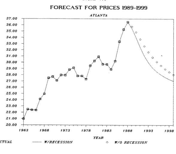
exceptions are Atlanta and Minneapolis, where, over the eleven year forecast period, prices trend downward and

permits trend upward. In Denver, permits initially rise but then trend downwards, ending the millennium below the 1988 level, while prices end the forecast period slightly above the 1988 level.

The permit equations for Atlanta and Minneapolis do not include price variables, which accounts for the fact that the permit forecasts do not move in the same direction as the price forecasts. In our regression analyses for Atlanta and Minneapolis, RPRICE and/or DRPRICE were insignificant and/or unexpectedly negative.

The "nonrecession" forecast of both prices and permits is generally higher than the "recession" forecast. However, this is not always the case.

Obviously, the forecast results are a function of the estimated equations and the forecast inputs. In Chapter THREE we discussed the fact that the coefficients of RPRICEt-1 in the price equations for Baltimore and

Philadelphia are greater than 1.00 and the resulting problem. We did make a forecast of prices and permits for these two cities using equations that did not include RPRICEt-l'

However, the results were bizarre oscillations of prices and permits. At the same time, the forecast results that we have included for these cities, using price equations with

RPRICEt-₁ coefficients greater than 1.00, are certainly suspect.

The forecast inputs are also questionable. They are based upon Wharton's year-old forecast and generally predict growth in employment, income, and population throughout the forecast period, except in Philadelphia and in Cleveland, where population decline is predicted from 1992-1997 for the former and from 1987-1992 for the latter. Our recession scenario only lasts for the first two years of the forecast and assumes no growth in employment and income during these years. The forecast for Boston, for example, would look quite different if income and employment were stable or

declining rather than increasing throughout the period. Our assumptions of stable mortgage and inflation rates are also unrealistic and affect the forecast results.

Following is a description of the forecast for each metropolitan area in historical context.

THE DENVER MARKET

Population, employment, and personal income grew

substantially from 1960 to 1988. Population increased from 879,500 to 1,663,800 (89%); employment grew from 305,183 to 792,900 (160%); real personal income per capita rose from $10,020 to $16,930.

its position relative to the other cities we studied. Denver was number 11 in 1963 and 9 in 1988, reflecting lower prices than 10 of the 14 cities in 1963 and lower prices than 8 of them in 1988. Denver had its highest real price percentage increase in 1983 (29% real, 33% nominal) and reached a price peak in 1986 ($42,610 real, $153,000 nominal). Real prices increased by 68% from 1963 to 1988.

In 1987, however, employment declined by almost 3%. This decline continued in 1988, though at a slower rate

(1.1%). Since 1960, employment had previously declined only

once, in 1975. Population grew at its slowest rate, in 27 years in 1987 (.54%) and in 1988 showed almost no improvement with a .60% increase. Real personal income per capita,

however, increased during this period, but at a snail's pace. In the 1960's and 1970's increases of 3% to 5% in real

personal income per capita were not uncommon. For 1984 through 1988 the rates of change were 4.05%, .67%, .06%,

.56%, and -3.04 respectively. In 1987 and 1988 real housing prices declined substantially (by 11.42% in 1987 and 9.55% in

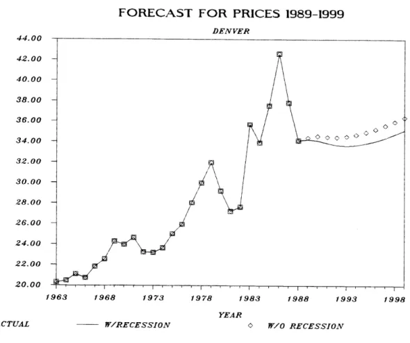
1988) so that prices in 1988 were slightly below 1983 levels. We forecast a modest price rise in Denver from 1989 to 1999, although with a dip in the early 1990's. Permits are projected to increase dramatically in 1989 from their 1988

trough but to fall back in the 1990's. The turnaround in the projected 1989 prices and permits from the steep decline of

1987 and 1988 is attributable to the positive forecast of employment (1.3%) income (1.5%) and population (1.0%) growth that we are using for 1989-1992.

FIGURE 4.1 44.00 42.00 40.00 38.00 36.00 34.00 32.00 30.00 28.00 26.00 24.00 22.00 20.00 E ACTUAL

FORECAST FOR PRICES 1989-1999 DENVER 1963 1968 1973 1978 1983 1988 1993 1998 YEAR W/RECESSION o W/0 RECESSION FORECAST 18 17 16 15 14 13 12 11 10 9 8 7 6 5 4 3 E ACTUAL FOR PERMITS 1989-1999 DENVER 1963 1966 1969 1972 1975 1978 1981 1984 1987 1990 1993 1996 1999 YEAR

W/RECESSION o W/O RECESSION 42

THE HOUSTON MARKET

Houston, as expected, given the depressed state of the region, underwent declines in real housing prices five times

in the 1980's (1981, 1982, 1984, 1985, 1987, and 1988),

despite a 336% increase in nominal prices from 1963 to 1988. Real prices in 1988 were actually near 1976 levels, and in

fact were lower than in 1971. Between 1963 and 1988 Houston real prices only rose 13%, the second lowest appreciation rate of the 14 cities we studied. In 1963, Houston was near the top of the "priciest" cities in our study, but by 1988 had dropped to eleventh place.

Houston's population grew rapidly and continually until 1984 when growth dropped precipitously (from 5.5% in 1982 to 2.6%, .61%, 1.75%, 1.31%, 1.19%, and .25% from 1983 to 1988). Total employment suffered its first decline since 1960

(6.17%) in 1983 and two subsequent declines in 1986 and 1987. In 1988 there were fewer people working in Houston than there were in 1981. Real personal income per capita declined 5

times during the 1980's, dropping twice to nearly 1976 levels.

Homebuilding, which soared from 3,231 units in 1974 to 16,949 units in 1975 and continued at an even greater pace, adding between 19,000 and 29,000 units per year until 1982, declined to under 7,000 units per year in 1985, with a low of 5,849 units in 1986.

We forecast an increase in prices and permits in Houston in the 1990's, although prices will dip in 1989 and permits will dip through 1991. Prices are a function of ESTK, USER2, and RPRICEt-1 while permits are a function of population, stock, lagged permits, and the mortgage rate. Our forecast of slow but steady growth in employment of 1.7% per year from 1989 to 1992 and 2.6% per year from 1992 to 1999, compared to fast growth in the 1960's and 1970's followed by swings from slow growth to fast decline in the 1980's, accounts for the steady, but slow, growth in prices in our forecast period, compared to the more dramatic fluctuations in the data. Our

forecast of population growth of 1.2% per year from 1989 to 1992 and of 1.3% per year from 1992 to 1999, compared with the higher growth rates of the pre-1984 period and the low, but fluctuating, rates after that, accounts for the forecast

FIGURE 4.2

FORECAST FOR PRICES 1989-1999

HOUSTON

1963 1968 1973 1978 1983 1988 1993 1998 YEAR

W/ RECESSION 0 W/ RECESSION

FORECAST FOR PERMITS 1989-1999

HOUSTON 1963 1966 1969 1972 1975 1978 1981 1984 1987 1990 1993 1996 1999 YEAR W/RECESSION 0 W/ RECESSION 32.00 31.00 30.00 29.00 28.00 27.00 26.00 25.00 24.00 23.00 22.00 21.00 f ACTUAL f ACTUAL

SAN FRANCISCO MARKET

While San Francisco had the distinction in 1988 of being the most expensive city in our study, having risen from

second place in 1963, 4 other cities experienced larger

percentage changes in real prices during the 1963-1988 period (Baltimore--97%, Boston--122%, Los Angeles--102%, and

Philadelphia--114%) compared to San Francisco's 95% increase. Real prices did not rise continuously in San Francisco, but declined in 1968, 1971, 1981, 1983, and 1984.

Population grew steadily throughout the period, with annual growth averaging about .5% from 1968 to 1980 and 1.45% in the 1980's. Population declined only once, in 1961.

Likewise, real personal income per capita rose continuously, with only one decline, of .04%, in 1974.

From 1984 to 1988, new construction of single family homes was at the level of approximately 11,000 to 12,000 units per year. This level was similar to that reached in the late 1970's and came after a slump in housing

construction that occurred in the early 1980's, when permits ranged from 3,486 to 8,882 units for four years.

For San Francisco we forecast continued growth in prices through the 1990's and a slight growth in permits. Prices are a function of ESTK, USER2, RPRICEt-1 and WAGE. Since

employment is increasing at the rates of 1.9% and 2.0% per year and incomes at the rates of 2.5% and 2.1% per year,

fluctuating less, but in the same range, than in the data period, prices continue their upward trend. Permits are a

function of WAGE, SFPRMT t-, and MTGR. Since we are holding the mortgage rate constant, permits increase gradually along with the projected increases in income relative to

FIGURE 4.3

FORECAST FOR PRICES 1989-1999

SAN FRANCISCO

1963 1968 1973 1978 1983 1988 1993 1998

YEAR

o W/O RECESSION

FORECAST FOR PERMITS 1989-1999

SAN FRANCISCO

1963 1968 1973 1978 1983 1988 1993 1998

YEAR

W/RECESSION 0 W/O RECESSION

0~ 65.00 60.00 55.00 50.00 45.00 40.00 35.00 30.00 25.00 ] ACTUAL W/ RECESSION 0 ACTUAL

THE MINNEAPOLIS MARKET

Employment in Minneapolis more than doubled from 579,959 in 1960 to 1,318,000 in 1988, a 127% increase. Population, on the other hand, increased only 40% during this period. Per capita income in this area grew substantially during the early 1960's (5.5%, 1.23%, 7.25%, and 4.01% from 1960 to 1964) and 75.63% from 1960 to 1988. But WAGE did not

experience the same growth and was only 8.48% in 1988 higher than it was in 1960. During the 25 years, WAGE decreased fourteen times, sometimes precipitously. In 1988 WAGE declined 5.8%.

In 1988, Minneapolis had an average family size of 1.8, the second smallest of our cities. (In Boston family size

averaged 1.7 in 1988.)

Housing prices trended upwards, but changes were

characterized by periodic leaps and less dramatic retreats rather than by steady increases or cyclical rises and falls. For example, real prices rose 16.3% in 1969, 14.5% in 1975, 10.4% in 1978, and 22% in 1986, but fell 3.6% in 1971, 4.3% in 1976, 4.3% in 1980, 4.7% in 1982, and 6.1% in 1988.

Overall, real prices rose 70.5% from 1963 to 1988, after

falling back in 1987 and 1988 from a 1986 high, while nominal prices rose 560%. Minneapolis became slightly more expensive relative to our other thirteen cities. In 1963 it was number 10 but moved up two places to number 8 in 1988, placing it

near the middle of our sample. Permits fluctuated

dramatically, dropping 40% from 1968 to 1970 and rising 140% from 1970 to 1972. They reached their highest level in 1978 and were 36% higher in 1988 than they were in 1960.

We forecast continued decline in prices through the 90's, but at a lower rate than in 1987 and 1988, and rising permits (after an initial continuation in our recession

scenario of the actual 1988 decline.) Prices are a function of ESTK, USER2, and RPRICE t-1 Permits are a function of

WAGE, SIZE, MTGR, and SFPRMTt-i. Since prices were declining

in 1987 and 1988 and we are forecasting steady and modest gains in employment, 1.8% per year in 1989-92 and 1.9% per year in 1992-1999, compared to higher actual growth rates in

1987 and 1988, prices will continue their decline but at a slower rate. Permits are not a function of prices, and

lagged permits are not significant. This, combined with our forecast of steady income growth of 2.4% per year and 2.5% per year and slower growth in employment (which results in increased WAGE), will result in growth in permits.

Employment will also grow faster than population which will result in a continued decline in SIZE, which has a negative sign in Minneapolis. If our forecast were correct, permits would reach a high in 1999, even under our recession

scenario.

40.00 39.00 38.00 37.00 36.00 35.00 34.00 33.00 32.00 31.00 30.00 29.00 28.00 27.00 26.00 25.00 24.00 23.00 22.00 21.00 20.00 C ACTUAL 20 19 18 17 16 15 14 13 12 11 10 9 8 7 6 5 4 3 2 1 0 C ACTUAL FIGURE 4.4

FORECAST FOR PRICES 1989-1999 MINNEAPOLIS

1963 1968 1973 1978 1983 1988 1993 1998

YEAR

W/ RECESSION o W/0 RECESSION

FORECAST FOR PERMITS 1989-1999 MINNEAPOLIS

1963 1968 1973 1978 1983 1988 1993 1998

YEAR

THE PHILADELPHIA MARKET

Surprisingly, Philadelphia experienced the second largest overall increase in both real and nominal prices. From 1963 to 1988 real prices rose a total of 114% while nominal prices rose a phenomenal 729%. Philadelphia ranked as the least expensive city in 1963 but moved up to sixth place by 1988.

Population in Philadelphia declined steadily for 8 consecutive years from 1972 to 1979, despite some gains in employment, per capita income, and wages. During this time real housing prices fell twice and only gained 2% overall. Real housing prices fell again in 1981, 1982, and 1983, from

$23,060 to $20,610, but rose 14.1% during 1986, 16.4% during

1987, and 19% during 1988. Permits fluctuated dramatically,

reaching peaks in 1973, 1978, and 1986, and valleys in 1970, 1974, and 1981-82. The valleys correspond to periods of rapidly rising mortgage interest rates and the peaks to periods of growth in employment and/or wages, reinforced in 1986 by a precipitous drop in the mortgage interest rate.

In our forecast, prices are a function of ESTK,

RPRICEt-1 , MTGR, and DRPRICEt-1. Permits are a function of change in EMP, WAGE, DPRICE, MTGR, and SFPRMTt-1. As

discussed in Chapter Three, since the coefficient of lagged price in the price equation exceeds 1.00, the forecast

results are particularly suspect. Price is principally a

function of the previous year's prices, which increase after 1982. The slow but steady gains in employment that are

forecast for the 1990's contribute to the projected

acceleration of housing prices to unimaginable levels (281% of 1988 levels) by 1999. Permits are projected to rise in the 1990's in response to higher rates of income growth than employment growth (resulting in WAGE growth) and accelerating price increases. The projected flat 10% mortgage interest rate exceeds the lower rates of 1986 to 1988 and will result

140.00 130.00 120.00 110.00 100.00 90.00 80.00 70.00 60.00 50.00 40.00 30.00 20.00 10.00 l ACTUAL FIGURE 4.5

FORECAST FOR PRICES PHILADELPHIA

1963 1968 1973 1978 1983 1988 1993 1998

YEAR

W/ RECESSION 0 W/O RECESSION

FORECAST 22 21 20 19 18 17 16 15 14 13 12 11 10 9 8 7 6 5 E ACTUAL FOR PERMITS 1989-1999 PHILADELPHIA 1963 1968 1973 1978 1983 1988 1993 1998 YEAR

THE CLEVELAND MARKET

Cleveland holds the record for the longest continual population decline (17 years, from 1971 to 1987.) In 1988 Cleveland's population was smaller than in 1960. However, employment grew in 20 of the 28 years, for a total increase of 30% from 1960 to 1988. Wages stagnated after 1963: the 1988 wage was the same as the 1964 wage and 4% lower than the 1973 high.

Real housing prices fluctuated, reaching a high in 1971 and a low in 1985. In 1988, prices were 11% higher (the smallest increase of any city) than in 1963, but lower than in 1971. In 1963, Cleveland was the seventh most expensive city, but had fallen to last place by 1988. Real prices rose 12% in 1986, 3.3% in 1987, and 4% in 1988, after falling in 12 of the previous 21 years.

In 1960, permits reached a high of 9,000 for the entire period. However, despite the population decline, permits

fluctuated between approximately 4,000 and 6,000 units per year until 1979, reaching a peak of 6,400 in 1977, and then

fell to a markedly lower level, reaching a low of less than 1,300 in 1982, when mortgage rates peaked, before rising to above 4,000 in 1986 from 1980 until 1985. Permits declined again in 1987 and 1988.

In our forecast, price is a function of ESTK, USER2 and RPRICEt-1. Permits are a function of WAGE, SIZE, MTGR,

PERMITt-1, and DRPRICE. We forecast a steep decline in

prices through 1991 and then a steady rise through 1999. The steady price rise is a result of slow, but steady, growth in employment through the forecast period and a flat mortgage rate. The initial decline is partially a result of the projected initial increase in the mortgage interest rate. However, since our price equation does not account for a

large percentage of historic prices (the R2 is only .59), there is considerable and unexplained discontinuity of the forecast from the actual data. We forecast a continuing decline in permits until 1989 (1990 in the recession

scenario) followed by a rise through the 1990's. Permits will decline in 1989 in response to the decline in price and to the increase in mortgage rate but will increase through the 1990's in response to the projected increase in WAGE.

FIGURE 4.6

FORECAST FOR PRICES 1989-1999

CLEVELAND

1963 1968 1973 1978 1983 1988 1993 1998

YEAR

W/RECESSION o W/O RECESSION

FORECAST FOR PERMITS 1989-1999

CLEVELAND 1963 1968 1973 1978 1983 1988 1993 1998 YEAR W/RECESSION W/0 RECESSION 26.00 25.00 24.00 23.00 22.00 21.00 20.00 0 ACTUAL 0 ACTUAL