Quantitative Ion Character Activity
Relationships (QICARs)
Research Report No R-1262
March 2011
ii
Quantitative Ion Character Activity Relationships (QICARs)
Final Project Report
presented to
Inorganics Unit
Ecological Assessment Division
Science and Technology Branch
Environment Canada
Fontaine Building
200 Boulevard Sacré‐Cœur
Gatineau QC K1A 0H3
EC Contribution Agreement with the CNTC for 2010/2011
Report prepared by Séverine Le Faucheur Peter G.C. Campbell and Claude Fortin Institut national de la recherche scientifique, INRS‐Eau, Terre et Environnement 490 de la Couronne, Québec (Québec) Canada G1K 9A9 Research Report No R‐1262 March 2011 © 2011
iii
Table of contents
1 Background ... 1 2 Toxicity predictions – methods and results ... 2 2.1 Description of the studied elements... 2 2.2 Brief literature review of models used to predict metal toxicity ... 2 2.3 Results of the toxicity predictions ... 7 2.3.1 Wolterbeek and Verburg model ... 7 2.3.2 Kinraide model ... 22 2.3.3 Model comparisons and identification of the most problematic elements ... 23 3 Speciation predictions – methods and results ... 27 3.1 Brief literature review ... 27 3.2 Chemical equilibrium calculations for two typical Canadian surface waters ... 28 3.3 Calculated speciation of Bi, the lanthanides and the platinum group elements in two typical Canadian surface waters ... 30 4 Summary and recommendations ... 34 4.1 Predicted speciation ... 34 4.2 Predicted toxicity ... 35 4.3 Recommendations ... 35 5 Reference List ... 37 6 Appendices ... 39 6.1 Appendix 1 ... 40 6.2 Appendix 2 ... 44
iv
List of Tables
Table 1: Names and symbols of the studied elements. ... 2 Table 2: Physical and chemical properties of metals that have been used for predicting their toxicity. ... 3 Table 3: Compilation of the data‐poor elements characteristics used in equations 2, 4 and 5. ... 6 Table 4: Limits within which the Wolterbeek and Verburg model is applicable. ... 7Table 5: Optimized constants (a0‐4) used in the Wolterbeek and Verburg (2001) model. ... 8
Table 6: Toxicity ranking of the first ten elements towards enzymes (1: most toxic element). ... 13 Table 7: Toxicity ranking of the first ten elements towards bacteria (1: most toxic element). ... 14 Table 8: Toxicity ranking of the first ten elements towards algae (1: most toxic element). ... 14 Table 9: Toxicity ranking of the first ten elements towards fungi (1: most toxic element). ... 15 Table 10: Toxicity ranking of the first ten elements towards protozoa (1: most toxic element). ... 16 Table 11: Toxicity ranking of the first ten elements towards copepods (1: most toxic element). ... 17 Table 12: Toxicity ranking of the first ten elements towards nematodes (1: most toxic element). ... 18 Table 13: Toxicity ranking of the first ten elements towards crustaceans in short‐term exposures (1: most toxic element). ... 19 Table 14: Toxicity ranking of the first ten elements towards crustaceans in long‐term exposure (1: most toxic element) ... 21 Table 15: Toxicity ranking of the first ten elements towards rainbow trout (1: most toxic element). ... 21 Table 16: Average metal position in the toxicity ranking tables (Tables 6‐15) with minimum and maximum values... 22
Table 17: Calculated consensus scale of softness (σcon), of toxicity (Tcon) and toxicity ranking (1: most toxic) of the studied metals... 23
Table 18: Compilation of the ion characteristics used in equations (2), (4) and (5) for the three “common” metals (Cd, Hg, Pb). ... 24
Table 19: Estimated toxic metal concentrations (M) calculated with the Wolterbeek and Verburg (2001) model. ... 25
Table 20: Calculated consensus scale of softness (σcon), of toxicity (Tcon) and toxicity ranking (1: most toxic) of the “common” and the predicted most toxic little‐studied metals. ... 26 Table 21: Chemical composition of the typical surface waters used to model the speciation of the elements of interest. ... 29 Table 22: Existence of stability constants for the complexes formed between the elements of interest and the dominant inorganic ligands in natural waters. ... 30 Table 23: Calculated inorganic speciation of the elements of interest (%) – Lake Ontario water, no DOM ... 32 Table 24: Calculated speciation of the elements of interest (%) – Lake Ontario water with DOM ... 33 Table 25: Calculated inorganic speciation of the elements of interest (%) – Canadian Shield water, no DOM ... 33 Table 26: Calculated speciation of the elements of interest (%) – Canadian Shield water with DOM ... 34
v
List of Figures
Figure 1: Predicted metal concentrations inhibiting fish carbonic anhydrase activity by 50%. ... 9 Figure 2: Predicted metal concentrations inhibiting glutamic oxalacetic transaminase activity by 20%. ... 9 Figure 3: Predicted metal concentrations inhibiting lactic dehydrogenase activity by 20%. ... 10 Figure 4: Predicted metal concentrations inhibiting fish acetylchlolinesterase activity by 50%. ... 10 Figure 5: Predicted metal concentrations inhibiting ribonuclease activity by 1%. ... 11 Figure 6: Predicted metal concentrations inhibiting ribonuclease activity by 50%. ... 11 Figure 7: Predicted metal concentrations inhibiting lipase activity by 1%. ... 12 Figure 8: Predicted metal concentrations inhibiting lipase activity by 50%. ... 12 Figure 9: Predicted metal concentrations inhibiting light emission by Vibrio fischeri (M) by 50%. ... 13 Figure 10: Predicted metal concentrations inhibiting light emission by Vibrio fischeri (N) by 50%. ... 14 Figure 11: Predicted metal concentrations reducing growth of S. capricornutum by 50%. ... 14 Figure 12: Predicted metal doses reducing germination of A. tenuis and B. fabea by 50%. ... 15 Figure 13: Predicted metal concentrations causing 50% mortality of S. ambiguum. ... 16 Figure 14: Predicted metal concentrations causing 50% mortality of C. abyssorum and E. padonus. ... 16 Figure 15: Predicted metal concentrations causing 50% mortality of C. elegans‐1. ... 17 Figure 16: Predicted metal concentrations causing 50% mortality of C. elegans‐2. ... 17 Figure 17: Predicted metal concentrations causing 50% mortality of D. magna‐1. ... 18 Figure 18: Predicted metal concentrations causing 50% mortality of D. magna‐2. ... 19 Figure 19: Predicted metal concentrations causing 50% mortality of D. hyalina. ... 19 Figure 20: Predicted metal concentrations reducing D. magna reproduction by 16% ... 20 Figure 21: Predicted metal concentrations reducing D. magna reproduction by 50% ... 20 Figure 22: Predicted metal concentrations causing 50% mortality of D. magna ... 20 Figure 23: Predicted metal concentrations causing 50% mortality of rainbow trout (Oncorhynchus mykiss) ... 21
1
1 Background
To deal with the less common metal‐containing compounds on the Domestic Substances List, Environment Canada will require information about the speciation and the inherent toxicity of many “data‐poor” elements. In this context, we explored the possible use of quantitative ion character‐activity relationships (QICARs) to predict the relative toxicity of these rarely studied elements in model natural waters and their speciation in solution. Such information should be invaluable for designing new toxicity tests for these elements and also for determining priorities based on which metals are likely to be most problematic.
Various quantitative structure‐activity relationships (QSARs) have been used for estimating the properties of "new" organic substances, with correlations using molecular properties ranging in sophistication from bulk properties through structure‐dependent techniques and quantum chemical considerations. Applications to metal compounds (salts and neutral inorganics) have been much less frequent, at least in part because the range of "new" inorganic substances is much narrower and the incentive to develop extrapolation tools has been less pervasive. The highest linear correlations for acute toxicity (including endpoints for EC50, reproductive inhibition, etc.) make use of one to two
parameters relating to metal ion characteristics such as electronegativity, ionisation potential, and/or the "hardness / softness" of the metal atom involved. For this reason, we refer here not to QSARs but rather to QICARs (quantitative ion character‐activity relationships), following the suggestion of Ownby and Newman (2003).
Possible uses of QICARs for metals and metal‐containing substances might include:
‐ As a screening tool, to review existing toxicity data and identify "outliers", i.e. toxicity values that depart from the QICAR predictions: These outliers might be LC or EC values that are abnormally low (and are driving regulation setting), or values that are unusually high; in either case, the QICARs could be used to flag values that merit further scrutiny.
‐ As an extrapolation tool, to estimate speciation (complexation) and the toxicity of little‐studied metals for which the existing geochemistry and toxicity data base is limited.
In the first phase of the work, in collaboration with Environment Canada personnel, we identified the range of elements to be investigated: Bi, the Platinum Group Elements and the Lanthanides. Note that in parallel two other CNTC working groups have reviewed the existing literature on the toxicity of the Platinum Group Elements (Claude Fortin and Feiyue Wang) and the Lanthanides (Mike Wilkie, Scott Smith and Jim McGeer). The results of their studies should be compared with the QICAR predictions presented in the present report.
The present project had two main components, the first of which focused on the toxicity of the elements of interest towards (aquatic) organisms. We reviewed the existing literature to choose the best models which permit the prediction of metal toxicity using metal ion characteristics, and we then ran the models and ranked the little‐studied elements in terms of their predicted relative toxicities. The second component related to the prediction of the speciation (complexation) of the little‐studied elements in natural waters. We screened the available geochemistry databases (Martell and Smith 2004; Academic Software 2001), looking for the complexation constants between the metals and the dominant inorganic ligands present in natural waters (i.e., hydroxide, chloride, carbonate, sulphate, fluoride), and then used chemical equilibrium models to predict the inorganic speciation of the elements of interest, i.e., their speciation in natural waters in the absence of natural organic matter.
2
2 Toxicity predictions – methods and results
2.1 Description of the studied elements
The names and symbols of the little‐studied metals are listed in Table 1. Except for bismuth, the studied elements belong to the platinum (Pt) and the lanthanide (La) groups. Table 1: Names and symbols of the studied elements. Name Symbol Bismuth BiPlatinum group Ruthenium Ru
Rhodium Rh Palladium Pd Osmium Os Iridium Ir Platinum Pt Lanthanide group Lanthanum Cerium La Ce Praseodymium Pr Neodymium Nd Promethium Pm Samarium Sm Europium Eu Gadolinium Gd Terbium Tb Dysprosium Dy Holmium Ho Erbium Er Thulium Tm Ytterbium Yb Lutetium Lu
2.2 Brief literature review of models used to predict metal toxicity
Although the use of QICAR to predict metal toxicity has not been nearly as widespread as the use of QSAR for organic molecules, several predictive models for metals can nevertheless be found in the environmental toxicology literature (see review by Walker et al. (2003)). These models are often based on one or two explanatory metal characteristics and applied to a range of toxicological responses (Kinraide 2009; Veltman et al. 2008; Ownby and Newman 2003; Wolterbeek and Verburg 2001; Tartara et al. 1997; Newman and McCloskey 1996; Barbich et al. 1986; Fisher 1986; Kaiser 1980; Jones and Vaughn 1978; Biesinger and Christensen 1972) – see Table 2 for a list of the physical and chemical properties of metals that have been used for predicting their toxicity.
3
Table 2: Physical and chemical properties of metals that have been used for predicting their toxicity.a
Metal properties Symbol Definition
Physical properties ‐ Atomic weight, atomic volume, density ‐ Melting point ‐ Polarizability ‐ Molar refractivity AW,V, MP A MR Properties that can be measured without changing the basic identity of the studied element. Electronic structure ‐ Position on the periodic table (atomic number) ‐ Electronic configuration (electron shells) ‐ Ionization energy (potential) ‐ Electron affinity AN IP, ∆IP E* AN is the number of protons in an atom, which defines its position in the periodic table. The electronic configuration represents the arrangement of electrons in the orbitals of an atom. The ionization energy (or potential) is the energy required to remove an electron from a gaseous atom or ion. ∆IP is the difference between the ion's IP with the oxidation number (OX) and the IP of the next lower oxidation number (OX‐1). The electron affinity is the energy change that occurs when an electron is added to a gaseous atom or ion. Redox capacities ‐ Oxidation number ‐ Standard electrode potential ‐ Electrochemical potential OX E0 ∆E0 Elements can lose electrons and be oxidized, or gain electrons to be reduced. E0 is the standard reduction potential. ∆E0 is the absolute value of the electrochemical potential between the ion and the first stable reduced state. Binding properties Indices ‐ Ionic radius ‐ Atomic radius, Covalent radius ‐ Electropositivity, electronegativity ‐ Ionic potential ‐ Ionic index ‐ Covalent index ‐ Covalent bond stability ‐ Log AN/∆IP, AN/∆IP ‐ Log of the first hydrolysis constant ‐ Hard and soft acids and bases (HSAB) theory IR or r AR, CR Xm Z/r Z2/r Xm2r ∆ß log KOH p, w Xm is the ability of an atom to attract electrons to itself in a chemical bond. Z is the ion's charge. Z2/r (polarizing power) is a measure of electrostatic interaction strength between an ion and a ligand. Xm2r is a measure for a metal ion of the importance of covalent interactions relative to ionic interactions. ∆ß is an empirical parameter, which reflects covalent bond stability of the metal‐ligand complex. HSAB theory categorizes the ions depending on their resistance to deformation in response to electric forces. a Properties indicated in bold are those used in the models that we have selected for QICAR toxicity predictions for the little‐studied elements.
4
Among the ion properties compiled in Table 2, the binding tendencies or ligand preferences of the different metals have been used successfully in several models. In contrast to the other characteristics, they define the ion with respect to its interactions with potential biotic ligands. For example, hard ions (high p) or class A ions (high Z2/r) bind preferentially to O‐donor atoms whereas soft ions or class B ions
seek S‐donor ligands.
One of the first models was developed by Kaiser in 1980 to express 16% reproductive impairment in Daphnia magna induced by the exposure to 21 different metals (Kaiser 1980). The general equation was:
0 0 1log
2AN
pT
E
IP
(1)where pT is the negative logarithm of a metal ion concentration with a certain toxicity expressed in mol∙L‐1, AN is the metal's atomic number, IP is the difference between the ion's ionization potential with the oxidation number (OX) and the ionization potential of the next lower oxidation state (OX‐1), and E0 is the absolute value of the electrochemical potential between the ion and the first stable reduced state. The values of α0, α1 and α2 depended on ion class or category, the organisms and the
tested endpoints. Further studies showed that this model was also effective in predicting express acute EC50 values for nine metals for a marine bacterium (Newman and McCloskey 1996) but gave variable
results for the response of Caenorhabditis elegans to metal exposure (Tartara et al. 1997) (note that AN/ΔIP was used instead of log (AN/ΔIP)). Wolterbeek and Verburg (2001) developed a more robust model, also based on fixed metal properties, by modelling toxicity results from 30 literature data sets, which varied widely in exposure times, test organisms, effects and effect levels. We used this as our first tested model; its general equation is:
0
0 1 2log
10 3 m 4log
10AR
pT
a
a E
a
IP a X
a
AW
(2) The definition of E0 is similar to that in equation 1, whereas IP is the ion's ionization potential at the oxidation state (OX), Xm the electronegativity, AR the atomic radius and AW the atomic weight. These metal properties are generally easily available and, in contrast to Kaiser's original model, metals do not need to be separated into basic classes (A, B, intermediate) to model toxicity. Moreover the relative contribution of each parameter to the calculated toxicities allows some mechanistic understanding of metal toxicity.
The second selected model is a more recently published equation, which uses a "consensus scale of softness" (con) and a "consensus scale for toxicity" (Tcon) to predict the toxicity of 92 ions (Kinraide
2009). Softness parameters have been extensively used in recent years, with more or less success, to model the toxicity of metal ions (Walker et al. 2003; Ownby and Newman 2003; Tartara et al. 1997; Newman and McCloskey 1996; Williams and Turner 1980; Jones and Vaughn 1978). One of the most studied has been the softness parameter as defined by Ahrland (1968), p, with:
( ) ( ) ( ) p CBE F CBE I CBE F (3)where CBE(F) and CBE(I) are the coordinate bond energy of the metal‐fluoride and metal‐iodide complexes, respectively. Based on this definition, p reflects the ability of a metal ion to give up its
5
valence electron, i.e. to form a covalent bond (Jones and Vaughn 1978). Kinraide constructed the consensus scale of softness, con, from eight published scales of softness, such as p, as well as from the logarithm of the solubility products of metal sulphides and the negative logarithm of the stability constant for metal ion binding to seven soft ligands. These different scales were normalized and averaged to obtain a consensus constant defined as:
0
con
aE I
pb
Metal (4)where E0 is the electrode standard potential, Ip the first ionization potential of the metal and Metal is the bulk metal density. As in the first model, these three ion characteristics are easily retrievable. The calculated constants a and b are 0.0607 and 0.0454, respectively. A consensus scale of toxicity was derived from ten different toxicity studies1 and is described by the following equation:
con con con
T
a
b
Z cZ
(5) where Z is the ion charge, a=2.16, b=‐0.521 and c=0.0778. This equation implies that toxicity of a given ion depends on its charge and its softness. Based on our literature review of the various approaches that have been used to explain differences in toxicity among metals, we selected the Wolterbeek and Verburg (2001) model and the Kinraide (2009) model for use in our simulations of the toxicity of the data‐poor elements of interest. Our selection criteria were that the models had been developed and used with a sufficient number of metals, with a broad range of ion property values, and that they leant themselves to mechanistic interpretations (McKinney et al. 2000). From the cited literature, one can easily see that Newman and his co‐workers have been active in the modelling of metal toxicity in relation to ion characteristics. However, we have decided not to use any of their developed models because of the much smaller pool of studied metals compared to the two models described above. In Table 2, properties indicated in bold are those used in the models that we have selected for QICAR toxicity predictions for the little‐studied elements. The ion characteristics used in equations 2, 4 and 5, as compiled for the data‐poor elements of interest in the present study, can be found in Table 3. Most of these metal properties were retrieved from the Handbook of Chemistry and Physics (Lide 2004). Values that were not available in this handbook were obtained, when possible, from other sources. The ionization potential of Ir, electronegativity values of Eu(II), Tb(III) and Yb as well as the atomic radii of most of the elements were retrieved from Wolterbeek and Verburg’s original article. The atomic radii of Pm, Sm and Tm were found in Cordero et al. (2008). No values of electrochemical and ionization potentials were found for osmium; the same situation prevailed for electronegativity values for Pm. Accordingly, toxicity values for these two elements could not be calculated. An important limitation of the Wolterbeek and Vereburg model, as pointed out by the authorsthemselves, is that it can only be applied to metals whose properties (E0, IP, Xm, AR and AW) fall within a calibration matrix representing the minimum and maximum numerical values of these properties for the metals used in the calibration of the model. In other words, the metal ion parameters for the data‐ 1 Kinraide (2009) used three of the 30 datasets used by Wolterbeek and Verburg (2001), and added seven additional studies – see Appendix 1 for a list of all these studies.
6 Table 3: Compilation of the data‐poor elements characteristics used in equations 2, 4 and 5. Element Z AR (Å)a,b AW (g∙mol‐1)c Metal (g∙cm‐3)c ∆E0 (V)c IP (eV)a,c Xma,c E0 (V)c First Ip (eV)c Bi 3 1.46 208.98038(2)d 10.05 0.2 25.56 1.9 0.308 7.2856 Ru 2 3 1.33 1.33 101.07(2) 101.07(2) 10.65 10.65 0.455 0.249 16.76 28.47 2.2 2.2 0.455 0.2487 7.36050 7.36050 Rh 3 1.35 102.90550(3) 10.7 0.758 31.06 2.28 0.758 7.45890 Pd 2 1.38 106.42(1) 10.38 0.951 19.43 2.20 0.951 8.3369 Os 1.44 190.23(3) 20 ‐e ‐ 2.2 ‐ 8.4382 Ir 3 1.36 192.217(3) 19 1.156 27 2.2 1.156 8.9670 Pt 2 1.38 195.078(2) 19.77 1.18 18.563 2.2 1.18 8.9587 La 3 1.87 138.91 6.15 ‐2.379 19.1773 1.10 ‐2.379 5.5769 Ce 3 4 1.82 1.82 140.115(4) 140.115(4) 6.55 6.55 ‐2.336 1.72 20.198 36.758 1.12 1.12 ‐2.336 1.72 5.5387 5.5387 Pr 3 1.82 140.90765(2) 6.50 ‐3.1 21.624 1.13 ‐2.353 5.473 Nd 3 1.83 144.24(3) 6.89 ‐2.7 22.1 1.14 ‐2.323 5.5250 Pm 3 1.99 (145) 6.50 ‐2.6 22.3 ‐ ‐2.30 5.582 Sm 3 1.98 150.36(3) 7.16 ‐1.55 23.4 1.17 ‐2.304 5.6436 Eu 2 3 1.98 1.98 151.964(1) 151.964(1) 5.13 5.13 ‐2.812 ‐0.36 11.241 24.92 1.15 1.15 ‐2.812 ‐1.991 5.6704 5.6704 Gd 3 1.79 157.25(3) 7.4 ‐2.279 20.63 1.20 ‐2.279 6.1501 Tb 3 1.76 158.92534(2) 7.65 ‐2.28 21.91 1.20 ‐2.28 5.8638 Dy 3 1.76 162.50(3) 8.37 ‐2.6 22.8 1.22 ‐2.295 5.9389 Ho 3 1.75 164.93032(2) 8.34 ‐2.8 22.84 1.23 ‐2.1 6.0215 Er 3 1.74 167.26(3) 8.86 ‐3.0 22.74 1.24 ‐2.331 6.1077 Tm 3 1.90 168.93421(3) 8.56 ‐2.2 23.68 1.25 ‐2.319 6.18431 Yb 3 1.94 173.04(3) 6.21 ‐1.05 25.05 1.25 ‐2.19 6.25416 Lu 3 1.72 174.967(1) 9.3 ‐2.28 20.9594 1.0 ‐2.28 5.4259
a Wolterbeek and Verburg (2001); b Cordero et al. (2008); c Lide (2004) – the absolute values of ∆E0 are used in the simulations ; d In column 4, the final number (in parentheses) represents an uncertain value; e The symbol "‐" means that no data were
7
poor elements of interest should fit within this calibration matrix. The limits within which the Wolterbeek and Verburg model is applicable are shown in Table 4. Fortunately, all of the elements of interest in the present study fall within these limits.
Table 4: Limits within which the Wolterbeek and Verburg model is applicable.
Minimum Properties Maximum
0 (Ge4+) E0 3.045 (Li+)
3.89390 (Cs+) IP 119.203 (Mn7+)
0.79 (Cs) Xm 2.55 (Se)
0.006986 (Bi) AR/AW 0.218989 (Li)
Note: The values are for the elements in parentheses, which represent the limits within which the model is applicable. 2.3 Results of the toxicity predictions 2.3.1 Wolterbeek and Verburg model
Wolterbeek and Verburg (2001) present comparisons between observed toxicities and predicted toxicities for 30 different data sets, corresponding to different organisms and different toxicity endpoints (Table 4 in their paper). Professor Wolterbeek kindly communicated to us the optimized values of a0, a1, a2, a3, a4 that were obtained by fitting equation (2) to each of their data sets (Table 5;
the mice, rat and drosophila data sets were not used because these organisms were not considered to be sufficiently “aquatic”). We then used these values to calculate the predicted toxicities of our data‐poor elements, as applied to several organisms and several endpoints. The obtained results are presented below. Note that elements which appear below in bold in the text are those that occupy the first position in the toxicity ranking tables (i.e., the most toxic).
2.3.1.1 Enzyme inactivation
Inactivation of six different enzymes (fish carbonic anhydrase, glutamic oxalacetic transaminase,
lactic dehydrogenase, fish acetylchlolinesterase, ribonuclease and lipase) by the elements of interest
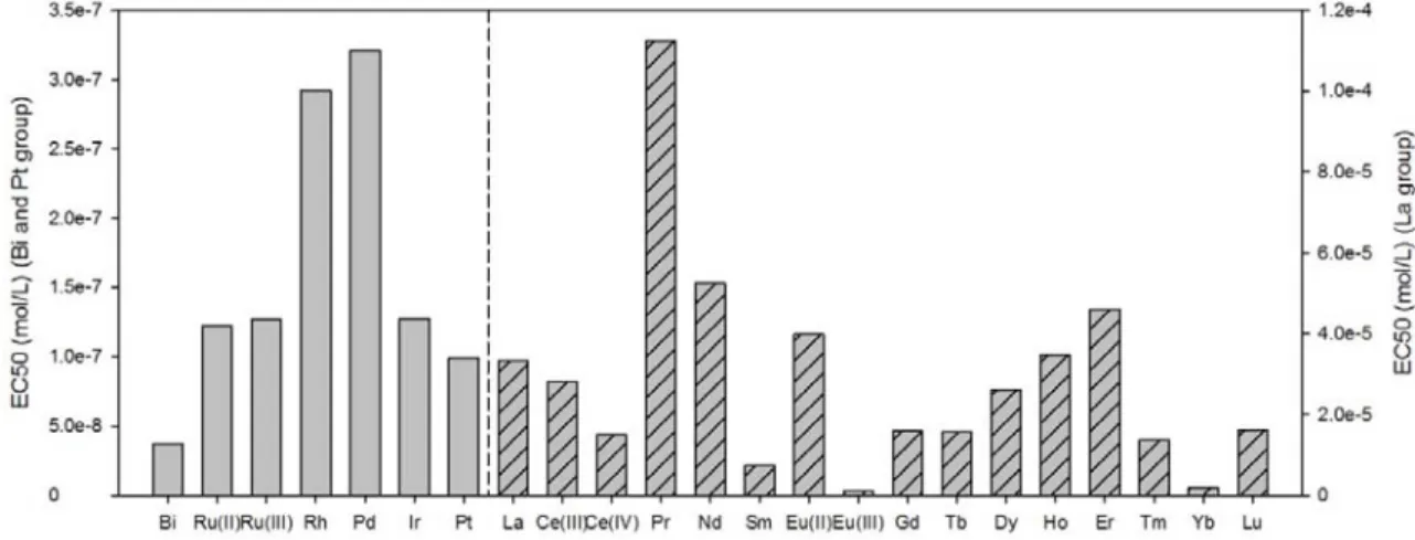
has been predicted with the present model (Figures 1 to 8). For three of these six studied enzymes (fish carbonic anhydrase, fish acetylchlolinesterase and lipase), the ten most toxic elements belong to the La group, with Er, Lu, Eu(II) or Pr (prediction with lipase was performed with two endpoints) as first toxicant (Table 6). For the fish carbonic anhydrase and acetylchlolinesterase (Figures 1, 4), the range of inactivating concentrations is very narrow for these first elements. For example, fish
carbonic anhydrase is inactivated at 2.6 x 10‐5M with Er (first element) to 5.1 x 10‐5M with Gd (10th
element) (Figure 1). The first element of the La group in the toxicity ranking for the same enzyme is Ir with a predicted concentration close to the range for the first ten elements (5.9 x 10‐5 M; 11th
element). For the lipase enzyme, the range of inactivating concentration of the first ten elements is wider by about one order of magnitude (Figures 7, 8). The first element of the Pt group in the toxicity ranking is Pt (15th and 16th) with an inactivating concentration of about 25 and 500 times higher than the most toxic element of the La group, for the endpoints I1 and I50, respectively. For the three other
enzymes (glutamic oxalacetic transaminase, lactic dehydrogenase and ribonuclease), the first ten elements belong to the Pt and La group, with Pt being predicted to be the most toxic metal for these enzymes (Table 6). The other members of the group of five most toxic metals are Ru(II), Pd, Ir and Rh. Europium(II), which is a La group element, also ranks in the first five metals with an inactivating concentration about three times higher than Pt for lactic dehydrogenase and ten times higher for
8
Table 5: Optimized constants (a0‐4) used in the Wolterbeek and Verburg (2001) model.
Target Enzyme or Species Exposure time R2 Effect n a0 a1 a2 a3 a4
Enzymes Fish carbonic anhydrase 0.69 I50 21 ‐2.357 0.217 1.057 ‐0.512 ‐2.768 Glutamic oxalacetic transaminase 0.80 I20 16 0.540 0.325 ‐2.918 1.799 ‐1.251 Lactic dehydrogenase 0.89 I20 15 0.543 0.138 ‐2.188 0.611 ‐2.106 Fish acetylcholinesterase 0.63 I50 17 1.525 0.076 ‐0.360 ‐0.819 ‐1.716 Ribonuclease 0.70 I1 14 2.046 0.645 ‐2.610 2.253 ‐0.171 Ribonuclease 0.64 I50 14 ‐1.187 0.792 ‐0.503 1.815 ‐0.242 Lipase 0.71 I1 17 3.027 1.053 ‐2.348 ‐0.968 ‐2.834 Lipase 0.73 I50 14 0.190 1.559 ‐1.248 ‐1.796 ‐3.659 Bacteria Vibrio fischeri (M) 15 m 0.93 EC50 20 ‐1.535 ‐0.533 ‐0.382 2.185 ‐1.555 Vibrio fischeri (N) 15 m 0.97 EC50 9 ‐34.032 1.990 15.305 4.278 ‐5.844 Algae Selenastrum capricornutum 96 h 0.99 EC50 9 1.677 ‐0.775 ‐0.782 0.792 ‐2.554 Fungi Alternaria tenuis 18 h 0.72 ED50 22 ‐4.214 ‐0.066 2.399 2.119 ‐0.819 Botrytus fabea 18 h 0.83 ED50 22 ‐2.076 ‐0.406 1.454 1.767 ‐0.875 Protozoans Spirostomum ambiguum 24 h 0.83 LC50 11 4.049 1.227 1.275 1.296 2.216 Spirostomum ambiguum 48 h 0.84 LC50 11 4.020 1.218 1.266 1.287 2.201 Copepods Cyclops abyssorum 48 h 0.95 LC50 12 0.310 ‐0.679 0.012 ‐0.422 ‐2.698 Eudiaptomus padonus 48 h 0.92 LC50 12 3.345 ‐1.061 ‐0.911 ‐0.782 ‐2.439 Nematodes Caenorhabditis Elegans‐1 24 h 0.93 LC50 9 ‐20.444 0.869 12.080 0.677 ‐3.356 Caenorhabditis Elegans‐2 24 h 0.78 LC50 18 ‐3.888 0.316 1.062 1.341 ‐1.201 Crustaceans Daphnia magna 21 d 0.88 RI16 21 1.403 ‐0.942 ‐0.128 ‐0.397 ‐3.411 Daphnia magna 21 d 0.88 RI50 21 1.557 ‐0.961 ‐0.065 ‐0.544 ‐3.278 Daphnia magna 21 d 0.83 LC50 21 1.855 ‐0.950 0.217 ‐0.790 ‐2.913 Daphnia magna‐1 48 h 0.90 LC50 15 1.654 ‐1.016 ‐0.453 ‐0.707 ‐3.616 Daphnia magna‐2 48 d 0.71 LC50 22 2.511 ‐0.614 ‐0.846 0.022 ‐1.949 Daphnia hyalina 48 h 0.88 LC50 12 ‐0.207 ‐1.263 2.284 ‐2.757 ‐4.930 Fish Rainbow trout 96 h 0.91 TL50 9 6.273 1.110 ‐2.588 ‐5.098 ‐6.126 Ix: Inactivation ‐ toxicant concentration that reduces (enzyme) activity by x %; I1 values are taken to be the effect‐no effect threshold; EC50: Effective toxicant concentration that reduces a response of an organism by 50 %; LC50: Lethal toxicant concentration that kills half of organisms; RIx: Reproductive impairment – toxicant concentration that reduces reproductive ability of an organism by x %; TL50: Tolerance limit = toxicant concentration that causes the mortality of 50% of the test organisms.
9 Figure 1: Predicted metal concentrations inhibiting fish carbonic anhydrase activity by 50%. Figure 2: Predicted metal concentrations inhibiting glutamic oxalacetic transaminase activity by 20%.
10 Figure 3: Predicted metal concentrations inhibiting lactic dehydrogenase activity by 20%. Figure 4: Predicted metal concentrations inhibiting fish acetylchlolinesterase activity by 50%.
11 Figure 5: Predicted metal concentrations inhibiting ribonuclease activity by 1%. Figure 6: Predicted metal concentrations inhibiting ribonuclease activity by 50%.
12 Figure 7: Predicted metal concentrations inhibiting lipase activity by 1%. Figure 8: Predicted metal concentrations inhibiting lipase activity by 50%.
13
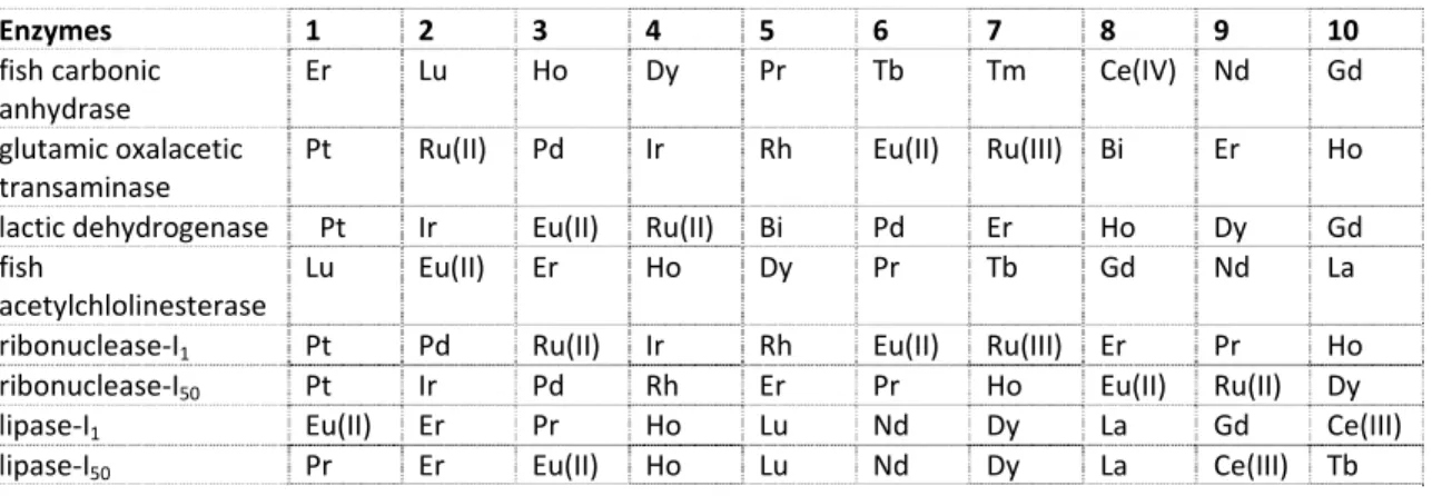
Table 6: Toxicity ranking of the first ten elements towards enzymes (1: most toxic element).
Enzymes 1 2 3 4 5 6 7 8 9 10
fish carbonic anhydrase
Er Lu Ho Dy Pr Tb Tm Ce(IV) Nd Gd glutamic oxalacetic
transaminase
Pt Ru(II) Pd Ir Rh Eu(II) Ru(III) Bi Er Ho lactic dehydrogenase Pt Ir Eu(II) Ru(II) Bi Pd Er Ho Dy Gd fish
acetylchlolinesterase
Lu Eu(II) Er Ho Dy Pr Tb Gd Nd La ribonuclease‐I1 Pt Pd Ru(II) Ir Rh Eu(II) Ru(III) Er Pr Ho
ribonuclease‐I50 Pt Ir Pd Rh Er Pr Ho Eu(II) Ru(II) Dy
lipase‐I1 Eu(II) Er Pr Ho Lu Nd Dy La Gd Ce(III)
lipase‐I50 Pr Er Eu(II) Ho Lu Nd Dy La Ce(III) Tb
2.3.1.2 Bacteria
Effects of our data‐poor elements on Vibrio fischeri (EC50) were modelled using two sets of a0‐4
parameters (Table 5). The effective concentration, EC50, corresponds to the concentration resulting in a 50% decrease of bacterial luminescence after 15 min of exposure to the metals. As was done by Wolterbeek and Verburg (2001), the two series of predicted toxicities were called V. fischeri (M) (for data from McCloskey et al. (1996)) and V. fischeri (N) (for data from Newman and McClosey (1996)). These two studies differed in the number of metals used to construct the models (nine in Newman and McCloskey (1996) and 20 in McCloskey et al. (1996)) and also in the exposure conditions (marine conditions in Newman and McCloskey (1996) and freshwater conditions in McCloskey et al. (1996). In both cases, the authors calculated the speciation of their metals and expressed the metal concentrations in terms of the free metal ion.
Bismuth and the elements of the Pt group are the most toxic for V. fischeri (M) with EC50 values about
1000 times lower than those of the La group (except for Eu(III) and Yb, which have an EC50 about 100
times higher) (Figure 9). The most toxic element is Ru(III) followed by Pt, Ru(II), Ir and Rh with a narrow range of predicted EC50s from 3.3 x 10‐6 M to 4 x 10‐6 M (Table 7). Bismuth is the next element
after Rh with an EC50 of 4.7 x 10‐6M. In V. fischeri (N), Ir and Rh are the most toxic metals with very
low EC50s of 7.0 x 10‐13 M and 8.6 x 10‐12 M, respectively (Figure 10). The third to the sixth elements in
the ranking are Pt, Er, Ce(IV) and Ho with EC50s between 1.9 and 7.3 x 10‐10 M. The following metals in
the toxicity ranking have predicted EC50s that are about 1000 times higher, starting with Ru(II) at 9.7
x 10‐7 M.
14 Figure 10: Predicted metal concentrations inhibiting light emission by Vibrio fischeri (N) by 50%. Table 7: Toxicity ranking of the first ten elements towards bacteria (1: most toxic element). 1 2 3 4 5 6 7 8 9 10
V. fischeri M Ru(III) Pt Ru(II) Ir Rh Bi Pd Eu(III) Yb Sm
V. fischeri N Ir Rh Pt Er Ce(IV) Ho Ru(II) Bi Dy Pr
2.3.1.3 Algae
Growth inhibition by the studied elements was predicted for the unicellular green alga, Selenastrum
capricornutum (now known as Pseudokirchneriella subcapitata). Bismuth and Pt with EC50s of 3.7 x
10‐8 M and 9.9 x 10‐8 M, respectively, are the most toxic elements for the alga, followed by other
elements of the Pt group (Figure 11, Table 8). The most toxic element in the La group is Eu(III) (8th;
EC50=9.3 x 10‐7 M), followed by Yb (9th; EC50=1.8 x 10‐6 M) and Sm (10th; EC50=7.3 x 10‐6 M).
Figure 11: Predicted metal concentrations reducing growth of S. capricornutum by 50%. Table 8: Toxicity ranking of the first ten elements towards algae (1: most toxic element). 1 2 3 4 5 6 7 8 9 10
15
2.3.1.4 Fungi
Metals of the Pt group and Bi are predicted to be the most toxic elements for two species of fungi (Alternaria tenuis and Botrytus fabea) (Figure 12). Rhodium, Ir and Ru(III) are ranked as the three first toxicants in the toxicity ranking with an ED50 range between 2.0 x 10‐6 M and 4.9 x 10‐6 M (Table
9). Cerium(IV) (8th) and Eu(III) (8th) are the most toxic metals of the La group with ED50 values 100
times higher than for elements of the Pt group, with a concentration of 4.5 x 10‐4 M (A. tenuis) and 3.2 x 10‐4 M (B. fabea), respectively. Figure 12: Predicted metal doses reducing germination of A. tenuis and B. fabea by 50%. Table 9: Toxicity ranking of the first ten elements towards fungi (1: most toxic element). 1 2 3 4 5 6 7 8 9 10
A. tenuis Rh Ir Ru(III) Pt Pd Bi Ru(II) Ce(IV) Yb Tm
B. fabea Ru(III) Rh Ir Bi Pt Ru(II) Pd Eu(III) Yb Ce(IV)
2.3.1.5 Protozoa
From the model calculations, the protozoan Spirostomum ambiguum is expected to be more impacted by elements belonging to the La group than those of the Pt group and Bi after 24 and 48 hours of exposure (Figure 13). The first ten metals in the toxicity ranking are similar after 24 and 48 h of exposure with LC50 values of Pr, Er and Ho ranging from 1.7 x 10‐7 M to 4.1 x 10‐7 M (Table 10).
Rhodium is the most toxic element in the Pt group (12th position) with a LC50 of 2.4 x 10‐6 M.
16 Figure 13: Predicted metal concentrations causing 50% mortality of S. ambiguum. Table 10: Toxicity ranking of the first ten elements towards protozoa (1: most toxic element). 1 2 3 4 5 6 7 8 9 10
S. ambiguum Pr Er Ho Nd Dy Eu(II) La Ce(III) Tm Tb
2.3.1.6 Copepods
Metal concentrations leading to 50% mortality (LC50) were modelled for Cyclops abyssorum and
Eudiaptomus padonus (Figure 14). In both organisms, Bi is predicted to be the most toxic element
with a LC50 of 6.2 x 10‐6 M and 2.4 x 10‐6 M for C. abyssorum and E. padonus, respectively.
Europium(III) ranks in second place in both copepods but with a much higher concentration for C.
abyssorum (LC50=2.1 x 10‐5 M) than for E. padonus (4.1 x 10‐6 M). The next elements in the ranking
list are Ir, Pt, Yb, Ru(III), Ru(II), Rh, Sm and Pd; their position in the toxicity ranking table depends on the studied copepods (Table 11). Figure 14: Predicted metal concentrations causing 50% mortality of C. abyssorum and E. padonus.
17
Table 11: Toxicity ranking of the first ten elements towards copepods (1: most toxic element).
1 2 3 4 5 6 7 8 9 10
C. abyssorum Bi Eu(III) Ir Pt Yb Ru(III) Ru(II) Rh Sm Pd
E. padonus Bi Eu(III) Yb Ru(III) Ru(II) Pt Ir Sm Pd Rh
2.3.1.7 Nematodes
Toxicity (LC50) of the studied elements towards Caenorhabditis elegans was modelled using two sets
of a0‐4 parameters, designated as C. elegans‐1 and ‐2 (Figures 15, 16). In the first series of toxicity
data (Figure 15), Ce(IV) is predicted to be the most lethal element with an EC50 of 8.9 x 10‐9 M,
followed by metals from both the Pt and La groups, with Ir (EC50 of 2.8 x 10‐7 M) and Rh (7.9 x 10‐7 M)
ranking at second and third position, respectively (Table 12). In the second series of modelled toxicity data (Figure 16), the elements of the Pt group are more toxic than those of the La group with the first five elements being Ir (1st; LC
50=3.0 x 10‐4 M), Pt (2nd; LC50=4.3 x 10‐4 M), Rh (3rd; LC50=5.6 x 10‐4 M), Pd
and Ru(III) (Table 12). The first element from the La group is Er (8th) with a LC
50 about ten times
higher than Ir. Figure 15: Predicted metal concentrations causing 50% mortality of C. elegans‐1. Figure 16: Predicted metal concentrations causing 50% mortality of C. elegans‐2.
18
Table 12: Toxicity ranking of the first ten elements towards nematodes (1: most toxic element).
1 2 3 4 5 6 7 8 9 10
C. elegans‐1 Ce(IV) Ir Rh Er Ho Dy Pr Tm Nd Bi
C. elegans‐2 Ir Pt Rh Pd Ru(III) Bi Ru(II) Er Ho Dy
2.3.1.8 Crustaceans
Parameters (a0‐4) to model the toxicity of our studied metals towards crustaceans are available for
short‐ and long‐term exposures (Table 5).
Short‐term exposure
Metal concentrations leading to the death of 50% of the crustaceans after an exposure period of 48 h were modelled for Daphnia magna with two series of a0‐4 parameters, called D. magna‐1 and ‐2
(Table 5) and Daphnia hyalina (Figures 17 to 19). Bismuth is predicted to be the most toxic metal for both D. magna‐1 and ‐2 with LC50 values of 5.4 x 10‐8 M and 3.6 x 10‐6 M, respectively, whereas Bi is
in 2nd place in the toxicity ranking for D. hyalina (LC
50=7.1 x 10‐9M), for which the most toxic element
is Eu(III) (LC50 = 2.2 x 10‐9 M). Europium(III) is also predicted to be among the more toxic elements for
D. magna with a 2nd (LC
50=2.2 x 10‐7 M) and 6th place for the data series 1 and 2, respectively.
Platinum is the second most lethal element for D. magna‐2 with a LC50 of 1.1 x 10‐5 M. The third
element in the toxicity ranking table is Yb for D. magna‐1 (LC50=7.6 x 10‐7 M) and D. hyalina (LC50=1.5
x 10‐8 M), whereas it is Ru(II) for D. magna‐2 (LC50=1.2 x 10‐5 M). Iridium and Sm are common
elements present among the ten most toxic elements for the three daphnids (Table 13).
19 Figure 18: Predicted metal concentrations causing 50% mortality of D. magna‐2. Figure 19: Predicted metal concentrations causing 50% mortality of D. hyalina. Table 13: Toxicity ranking of the first ten elements towards crustaceans in short‐term exposures (1: most toxic element). 1 2 3 4 5 6 7 8 9 10
D. magna‐1 Bi Eu(III) Yb Pt Ir Ru(III) Ru(II) Sm Rh Pd
D. magna‐2 Bi Pt Ru(II) Ru(III) Ir Eu(III) Pd Yb Rh Sm
D. hyalina Eu(III) Bi Yb Ce(IV) Lu Sm Tm Tb Gd Ir
Chronic exposure
Three chronic toxicity endpoints (RI16, RI50 and LC50) in Daphnia magna were predicted with the
present model (Figures 20 to 22). Similar to the case for short‐term exposure, Bismuth and Eu(III) are also predicted to be the most toxic elements for D. magna for longer exposure times. Reduction of daphnid reproduction by Bi is predicted at 2.8 x 10‐8 M (RI
16) and 4.9 x 10‐8 M (RI50) whereas the
predicted LC50 value is 1.8 x 10‐7 M. Impacts of Eu(III) on the daphnids are predicted for
concentrations of 1.4 x 10‐7 M (RI
16), 2.1 x 10‐7 M (RI50) and 4.0 x 10‐7 M (LC50). Depending on the
toxicity endpoints, the next metals in the toxicity ranking table are Ir, Pt, Ru(III), Yb and Pt (Table 14).
20 Figure 20: Predicted metal concentrations reducing D. magna reproduction by 16% Figure 21: Predicted metal concentrations reducing D. magna reproduction by 50% Figure 22: Predicted metal concentrations causing 50% mortality of D. magna
21
Table 14: Toxicity ranking of the first ten elements towards crustaceans in long‐term exposure (1: most toxic element)
1 2 3 4 5 6 7 8 9 10
D. magna RI16 Bi Eu(III) Ir Pt Ru(III) Yb Ru(II) Rh Pd Sm
D. magna RI50 Bi Eu(III) Ir Ru(III) Pt Yb Ru(II) Rh Pd Sm
D. magna LC50 Bi Eu(III) Yb Ru(III) Ir Pt Ru(II) Sm Ce(IV) Rh
2.3.1.9 Fish
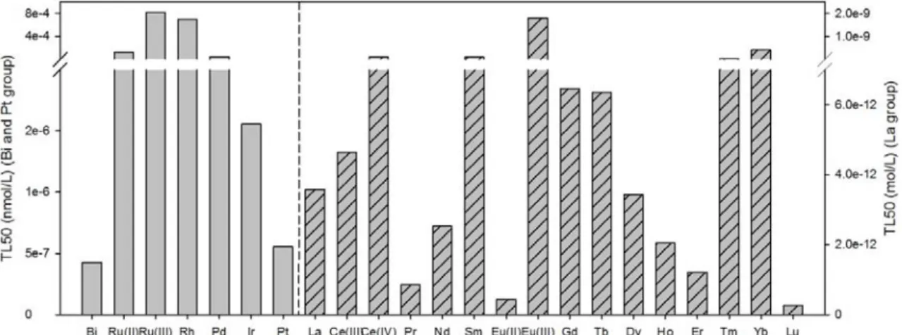
The elements of the La group are predicted to be more toxic for the rainbow trout than those of the Pt group and Bi (Figure 23; Table 15). The predicted TL50 values are very low for the first ten
elements, ranging from 2.6 x 10‐13 M (1st; Lu) to 6.3 x 10‐12 M (10th; Tb). The most toxic element of the Pt group has a modelled TL50 of 5.5 x 10‐7 M (Pt, 18th). Bismuth is 17th with a TL50 of 4.2 x 10‐7 M.
Figure 23: Predicted metal concentrations causing 50% mortality of rainbow trout (Oncorhynchus
mykiss)
Table 15: Toxicity ranking of the first ten elements towards rainbow trout (1: most toxic element).
1 2 3 4 5 6 7 8 9 10
O. mykiss Lu Eu(II) Pr Er Ho Nd Dy La Ce(III) Tb
2.3.1.10 General ranking
The estimated toxicity of our little‐studied metals towards aquatic organisms with the Wolterbeek and Verburg model depends on the organism, the exposure time and the measured effect. In other words, the ranking of an individual metal varies from one combination of toxicological endpoint and test organism to another. In order to conclude which metals could potentially be problematic among those studied, an average position for each metal has been calculated (Table 16).
Overall, the elements of the Pt group and Bi are predicted to be more toxic than those of the La group. Iridium is the metal with the lowest average position (i.e., the most toxic), which reflects the various toxicity rankings (Tables 6‐15) since Ir is present in 19 out of 23 rankings. Two enzymes (fish
carbonic anhydrase and lipase), protozoa and fish seem to be less sensitive to Ir than are the other
tested organisms. The second most toxic element is Pt, which is positioned 16 times out of 23 among the ten most toxic metals. In addition to the less sensitive endpoints mentioned for Ir, D. hyalina and
C. elegans‐1 are predicted to be less impacted by Pt than the other test organisms. Finally, Bi is
22 in the toxicity ranking tables. As in the case of Ir and Pt, enzymes, protozoa and rainbow trout are predicted to be the least sensitive targets for Bi. Table 16: Average metal position in the toxicity ranking tables (Tables 6‐15) with minimum and maximum values.
Ranking Element Average position SD minimum maximum
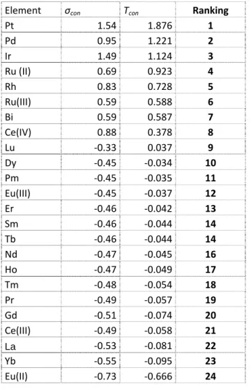
1 Ir 7.1 5.9 1 19 2 Pt 7.7 6.5 1 18 3 Bi 8.7 7.5 1 22 4 Rh 10.1 6.9 1 23 5 Ru(III) 10.3 7.5 1 23 6 Pd 11.2 6.4 2 22 7 Ru(II) 11.3 7.7 2 23 8 Er 11.3 8.1 1 22 9 Ho 11.4 6.5 3 21 10 Dy 11.6 4.8 4 18 11 Tm 11.9 2.4 7 17 12 Tb 12.2 2.5 6 15 13 Lu 12.3 6.0 1 22 14 Yb 12.5 6.5 3 22 15 Ce(IV) 12.7 5.3 1 23 16 Gd 12.9 2.4 8 17 17 Eu(III) 13.2 8.5 1 23 18 Pr 13.8 8.6 1 23 19 Sm 14.0 4.8 6 22 20 Nd 14.5 6.0 4 22 21 Eu(II) 14.8 8.5 1 23 22 Ce(III) 14.8 3.6 8 20 23 La 15.5 4.5 7 21 2.3.2 Kinraide model As described in section 2.2, the Kinraide (2009) model uses a consensus scale of softness and toxicity to describe metal toxicity. The main difference with the Wolterbeek and Verburg (2001) model is that the Kinraide approach does not provide an estimated toxic concentration for each metal; rather, it provides an overall toxicity ranking of the metals. Based on equations (4) and (5) and the needed metal characteristics (Table 3), the consensus scale of softness and toxicity have been calculated for the elements of interest (Table 17). The elements of Pt group are predicted to be more toxic than those of the La group due to a higher softness parameter. Bismuth is also estimated to be more toxic than metals form the La group.
23
Table 17: Calculated consensus scale of softness (σcon), of toxicity (Tcon) and toxicity ranking (1:
most toxic) of the studied metals.
Element σcon Tcon Ranking
Pt 1.54 1.876 1 Pd 0.95 1.221 2 Ir 1.49 1.124 3 Ru (II) 0.69 0.923 4 Rh 0.83 0.728 5 Ru(III) 0.59 0.588 6 Bi 0.59 0.587 7 Ce(IV) 0.88 0.378 8 Lu ‐0.33 0.037 9 Dy ‐0.45 ‐0.034 10 Pm ‐0.45 ‐0.035 11 Eu(III) ‐0.45 ‐0.037 12 Er ‐0.46 ‐0.042 13 Sm ‐0.46 ‐0.044 14 Tb ‐0.46 ‐0.044 14 Nd ‐0.47 ‐0.045 16 Ho ‐0.47 ‐0.049 17 Tm ‐0.48 ‐0.054 18 Pr ‐0.49 ‐0.057 19 Gd ‐0.51 ‐0.074 20 Ce(III) ‐0.49 ‐0.058 21 La ‐0.53 ‐0.081 22 Yb ‐0.55 ‐0.095 23 Eu(II) ‐0.73 ‐0.666 24 2.3.3 Model comparisons and identification of the most problematic elements The use of the models developed by Wolterbeek and Verburg (2001) and Kinraide (2009) allowed us to classify our little‐studied elements as a function of their potential toxicity towards aquatic organisms (Tables 16, 17). Both models predict that the elements of the Pt group as well as Bi should be more toxic than the elements of the La group. Iridium and Pt are expected to be the most potent metals among the studied elements, both ranking among the three most toxic metals for both models; Bi falls third in the Wolterbeek and Verburg ranking, whereas the second rank in the Kinraide scale is occupied by Pd. Thus, the four main elements that have been identified as potentially problematic for aquatic ecosystems on the basis of their inherent toxicity are Pt, Ir, Pd and Bi.
In order to get a better picture of the potential toxicity of these four selected elements, we have compared their estimated toxicity with that of three “common” metals (i.e., Cd, Hg and Pb). To this end, the ion characteristics of these “common” metals were compiled (Table 18) and applied in equations 2, 4 and 5. The results obtained with the Wolterbeek and Verburg model are presented in
Table 19, to which we have added Pt, Ir, Pd and Bi to facilitate the comparisons.
Our selected elements were found to be more toxic towards enzymes, bacteria, fungi, protozoa and nematodes than Cd, Hg and Pb. In only one of the eight enzymatic studies (fish acetylchlolinesterase)
24
was one of the "common" metals (i.e. Pb) found to be more toxic than Bi, Pd, Ir and Pt, with an I50
value (5.1 x 10‐4 M) close to those of Bi (6.6 x 10‐4 M) and Pt (9.0 x 10‐4 M). In contrast, Pt is predicted to be the most toxic element in six out of the eight enzymatic tests. Its inhibitory concentrations are very similar to those of Hg and Pb for glutamic oxalacetic transaminase and lactic dehydrogenase, and to that for Hg alone in lipase, whereas it is ten times lower than those of the three "common" metals for ribonuclease. Iridium is also predicted to be more toxic than Cd, Hg and Pb towards fish
carbonic anhydrase with an I50 value close to that of Hg. In V. fischeri M and N, Pt and Ir, respectively,
are also predicted to be more toxic than Cd, Hg and Pb. In V. fischeri M, the EC50 of Pt (3.2 x 10‐6 M) is
of the same order of magnitude as the EC50 of Pb (6.5 x 10‐6 M), whereas in V. fischeri N, Ir is found to
be much more toxic (7.0 x 10‐13 M) than Hg (1.8 x 10‐8 M), the most toxic of the "common" metals. Iridium is also predicted to be more toxic than Hg (most toxic element of the "common" metals) towards fungi ( 10 x) and nematodes ( 10 to 100 x), whereas Pd is predicted to be more toxic ( 10 x) than Hg (most toxic "common" element) in protozoa.
In algae, copepods and crustaceans, Pb is found to be more toxic than the selected little‐studied metals. However, its predicted toxic concentrations are very close to those of Bi. For example, in algae, the EC50 of Pb is 3.0 x 10‐8 M and the EC50 of Bi is 3.7 x 10‐8 M. In the copepod C. abyssorum,
the LC50 of Pb is 6.0 x 10‐6 M and LC50 of Bi is 6.2 x 10‐6 M. This tendency is also observed in
crustaceans. In fish, Cd, Hg and Pb are predicted to be more toxic than the selected little‐studied elements.
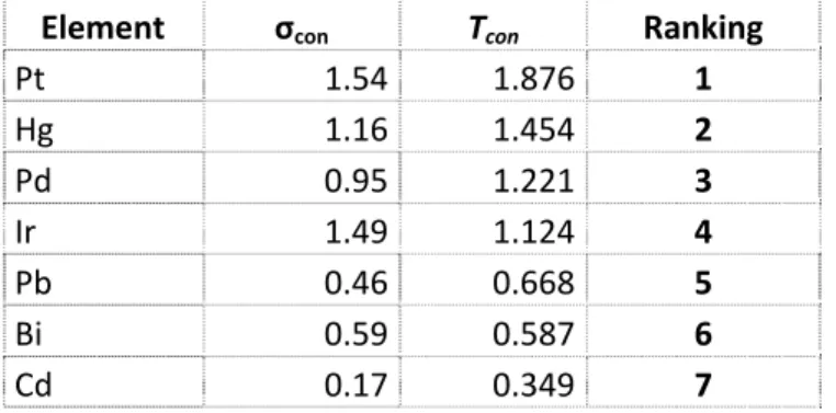
A similar exercise was carried out for the Kinraide (2009) model. The consensus softness and toxicity values for the "common" metals were calculated according to equation (5) and are presented in
Table 20. The values of our selected metals are included in the table to facilitate comparisons.
Platinum is predicted to be the most toxic element among all the studied metals, followed by Hg, Pd and Ir. Table 18: Compilation of the ion characteristics used in equations (2), (4) and (5) for the three “common” metals (Cd, Hg, Pb). Element Z AR (Å)a,b AW (g∙mol‐1)c Metal
(g∙cm‐3)c ∆E0 (V)c IP (eV)c Xma,c E0 (V)c
First Ip (eV)c Cd 2 1.48 112.4 8.65 ‐0.403 16.9083 1.69 ‐0.403 8.9938 Hg 2 1.48 200.59 13.7 0.851 18.756 1.9 0.851 10.4375 Pb 2 1.54 207.19 11.34 ‐0.1262 15.0322 1.8 ‐0.1262 7.41666
a Wolterbeek and Verburg (2001); b Cordero et al. (2008); c Lide (2004) – the absolute values of ∆E0
25 Table 19: Estimated toxic metal concentrations (M) calculated with the Wolterbeek and Verburg (2001) model. Bi Pd Ir Pt Cd Hg Pb Enzymes fish carbonic
anhydrase 6.8E‐05 4.9E‐04 5.9E‐05 8.6E‐05 4.3E‐04 7.9E‐05 1.3E‐04 glutamic oxalacetic
transaminase 2.4E‐03 3.9E‐04 4.1E‐04 1.3E‐04 3.3E‐03 6.5E‐04 8.9E‐04 lactic dehydrogenase 6.4E‐04 6.7E‐04 3.6E‐04 1.6E‐04 1.2E‐03 3.0E‐04 2.7E‐04 fish
acetylchlolinesterase 6.6E‐04 2.7E‐03 1.0E‐03 9.0E‐04 1.1E‐03 5.8E‐04 5.1E‐04 ribonuclease‐I1 7.1E‐04 2.7E‐05 4.2E‐05 1.5E‐05 5.9E‐04 1.2E‐04 3.4E‐04
ribonuclease‐I50 5.9E‐03 4.3E‐04 3.0E‐04 2.4E‐04 9.2E‐03 1.6E‐03 7.9E‐03
lipase‐I1 6.3E‐05 6.0E‐05 1.4E‐05 5.6E‐06 5.5E‐05 7.3E‐06 2.1E‐05
lipase‐I50 6.0E‐04 9.6E‐04 7.6E‐05 4.3E‐05 7.4E‐04 4.8E‐05 3.4E‐04
Bacteria
V. fischeri M 4.8E‐06 6.2E‐06 3.5E‐06 3.2E‐06 4.0E‐05 1.0E‐05 6.5E‐06
V. fischeri N 2.3E‐09 9.6E‐09 7.0E‐13 1.9E‐10 1.6E‐04 1.8E‐08 4.2E‐05
Algae
S. capricornutum 3.7E‐08 3.2E‐07 1.3E‐07 9.9E‐08 2.9E‐07 1.1E‐07 3.0E‐08
Fungi
A. tenuis 1.1E‐05 9.5E‐06 2.7E‐06 6.7E‐06 1.5E‐04 2.8E‐05 6.9E‐05
B. fabea 7.4E‐06 1.1E‐05 5.0E‐06 8.7E‐06 6.6E‐05 2.2E‐05 2.4E‐05
Protozoa
S. ambiguum‐24h 1.7E‐04 3.0E‐06 4.2E‐06 6.3E‐06 7.4E‐05 3.5E‐05 4.8E‐04
S. ambiguum‐48h 1.8E‐04 3.3E‐06 4.6E‐06 6.9E‐06 7.9E‐05 3.8E‐05 5.1E‐04
Copepods
C. abyssorum 6.2E‐06 1.4E‐04 3.8E‐05 4.0E‐05 3.9E‐05 2.0E‐05 6.0E‐06
E. padonus 2.4E‐06 9.0E‐05 4.6E‐05 3.5E‐05 8.7E‐06 1.0E‐05 1.2E‐06
Nematodes
C. elegans‐1 5.6E‐06 1.7E‐04 2.8E‐07 2.4E‐05 6.4E‐03 7.6E‐05 5.7E‐03
C. elegans‐2 1.6E‐03 1.0E‐03 3.0E‐04 4.3E‐04 8.6E‐03 1.4E‐03 4.3E‐03
Crustaceans
short‐term
D. magna‐1 5.5E‐08 4.3E‐06 8.9E‐07 8.0E‐07 5.1E‐07 2.6E‐07 3.8E‐08
D. magna‐2 3.6E‐06 2.7E‐05 1.5E‐05 1.1E‐05 1.2E‐05 7.8E‐06 2.4E‐06
D. hyalina 7.2E‐09 1.7E‐05 7.3E‐07 1.8E‐06 2.0E‐07 1.3E‐07 1.4E‐08
long‐term
D. magna RI16 2.3E‐08 1.2E‐06 2.6E‐07 2.6E‐07 2.5E‐07 1.1E‐07 2.1E‐08
D. magna RI50 4.9E‐08 2.8E‐06 6.2E‐07 6.4E‐07 4.6E‐07 2.4E‐07 4.4E‐08
D. magna LC50 1.8E‐07 1.0E‐05 2.6E‐06 2.9E‐06 1.3E‐06 9.3E‐07 1.7E‐07
Fish
O. mykiss 4.2E‐07 4.6E‐05 1.6E‐06 5.5E‐07 3.6E‐07 5.0E‐08 5.9E‐08
26
Table 20: Calculated consensus scale of softness (σcon), of toxicity (Tcon) and toxicity ranking (1: most
toxic) of the “common” and the predicted most toxic little‐studied metals.
Element σcon Tcon Ranking
Pt 1.54 1.876 1 Hg 1.16 1.454 2 Pd 0.95 1.221 3 Ir 1.49 1.124 4 Pb 0.46 0.668 5 Bi 0.59 0.587 6 Cd 0.17 0.349 7
27
3 Speciation predictions – methods and results
3.1 Brief literature review
To estimate the inorganic speciation of the metals of interest, one first needs the complexation constants for the metal and the dominant inorganic ligands present in natural waters, e.g. HO‐, Cl‐, SO42‐,
HCO3‐ and CO32‐, as extrapolated to an ionic strength I=0 (i.e., at infinite dilution). To that end, one of our
first challenges was to identify the stable oxidation states of the little‐studied elements in aqueous solutions. Lanthanides are predominantly trivalent with the exception of cerium and europium, which can exist as Ce(IV) and Eu(II) (Elderfield and Greaves 1982). Bismuth is also predominantly trivalent as are rhodium and iridium (Filella 2010; Richens 1997). Ruthenium exists as Ru(II) and Ru(III) whereas platinum and palladium are mainly present in the oxidation state (II) (Richens 1997). Osmium is a very complex element that has no characterised cationic aquo ions (Richens 1997). These oxidation states were used to guide the compilation of the relevant stability constant data for the metal complexes with inorganic ligands. Once compiled, the stability constant data can be used as input to a chemical equilibrium model2. Such models take into account the various reactions in which metal cations can participate. Examples include complexation reactions, oxidation and reduction reactions, and precipitation reactions: complexation reactions, e.g. 3 1 2 Dy HO DyOH precipitation reactions, e.g. 3 1 3 Dy 3 HO Dy(OH) (s) oxidation‐reduction reactions, e.g. 2 1 3 Fee Fe In addition, the models can be set up to take into account gas exchanges between the atmosphere and the aqueous solution: gas exchanges, e.g. 1 2 2 2 3 3 CO H OH CO H HCO
The models do not consider just one cation, but rather are able to solve the equilibrium equations simultaneously for all the cations and anions in solution. The process of solving chemical equilibrium problems involves the following steps (Schecher and McAvoy 2001): (i) selection of the chemical components that will define the system; (ii) definition of the chemical species that can be formed by these components; (iii) setting the total concentrations of the individual components; and (iv) solving the simultaneous equilibria. To perform these calculations, the model needs the equilibrium constant for each of the reactions to be considered; for each model, these constants are normally supplied as part of a default thermodynamic database that comes with the software package. Normally these
2