Dynamic modeling of vertical U-tube steam generators for operational safety systems

DYNAMIC MOI).ELING OF VEFRTICAl. U-TUIEI STEAM GENERIATO RS IOR OPERIAIONAL, SAFETI SYSTETMS

(Voi 11)

by

WALTF.R HERBERT ST'ROHMAYER

B. S. Rensselaer Polytechnic Institute

(Dec. 1976)

S. M. MNIassachlusetts

Institute of Technology

1978)

S UBMI ITI) TO T1 ll DI)'.PARTMr,.N'I' OF NUCI.lFAIR FNG1NFF'RING IN P.ARTIAL

FUuI.I.l.Ml'N' O 'TIlE RI:QUIR'MEN1I S FOR TIlE

I).GREE OF1 DOcTOR Oit PHIIosoPttY

at the

MASSACHIUSLETS I NSTII 'UI' OF TciCI tNOILOGY

August 1982

© Walter Herbert Strolimayer 1982

Signature of Author

Department ot'N

luclear Engineering

AuLgust 1982

Certified by_

'rofessor John E. Meyer

Accepted by

-

rroressor Allan F. Henry

Chainnan, Departmental Graduate Committee

DYNAMIC MODELING OF VERTICAL U-TUBE STEAM GENERATORS FOR OPERATIONAL SAFETY SYSTEMS

by

Walter Herbert Strohmayer

Submitted to the Department of Nuclear Engineering on August 25, 1982. in partial fulfillment of the requirements for the degree of Doctor of Philosophy

in Nuclear Engineering.

ABSTRACT

Currently envisioned operational safety systems require fast running computer models of major power plant components in order to generate reliable estimates of significant

safety-related parameters. The objectives of this research are to develop and to validate such a model for a vertical U-tube natural circulation steam generator.

The model is developed using a first principles appli-cation of the one-dimensional conservation equations of mass, momentum, and energy. Two-phase flow is treated by using the drift flux model. Two salient features of the model are the incorporation of an integrated secondary-recirculation-loop momentum equation and the retention of all nonlinear effects. The inclusion of the integrated loop momentum equation permits calculation of the steam generator water level. The use of a nonlinear model, as opposed to a linearized model, allows accurate calculation of steam gen-erator conditions for transients with large changes from nominal operating conditions.

The model is validated over a wide range of steady-state conditions and a spectrum of transient tests ranging from turbine trip events to a milder full-length control-element assembly drop transient. The results of the valida-tion effort are encouraging, demonstrating that the model is suitable for application to a broad range- of operational transients.

Execution speed of the model appears to be fast enough to achieve real-time execution on plant process computers. Real Time-to-CPU Time ratios for running the computer pro-gram on an Amdahl 470 V/8 computer range from 47 to 200, with integration time step sizes of 0.1 to 0.4 seconds, respectively. When the model is run on a Digital Equipment Corp. VAX 11/780 computer using an integration time step of 0.25 seconds, the Real Time-to-CPU Time ratio is 11.

Thesis Supervisor: John E. Meyer

Title: Professor of Nuclear Engineering

Thesis Reader: David D. Lanning

ACKNOWLEDGMENTS

I would like to express my heartfelt appreciation to my

thesis supervisor, Professor John E. Meyer, for his

inval-uable support, advice, and assistance. His willingness to discuss, at any time, topics related to this project has

made my association with him a privileged and rewarding

experience.

Thanks are also due to Professor David D. Lanning who served as the reader of this thesis and motivated the

ad-vanced control systems group.

I wish to express my gratitude to Professor Allan F. Henry for his encouragement throughout my stay at M.I.T.

The work was funded through the fellowship program t

The Charles Stark Draper Laboratory. This allowed me to work with a group of professionals who truly enriched my own

professional development. I wish to acknowledge: Dr. John

Hopps, for his support and advice; Mr. James Deckert for his

valuable comments, help, and advice during the research;

Dr. Jay Fisher, for his support and thoughtful suggestions,

particularly during the validation phase of the study; Dr.

Asok Ray, whose technical expertise and willingness to share his knowledge contributed in no small way to my education;

and, Mr. Renato Ornedo, for his advice, constructive

The RD-12 boiler data was acquired through the courtesy

of Mr. C.G. Mewdell of Ontario Hydro, and Mr. W.C. Harrison

of the Whiteshell Nuclear Research Establishment.

Thanks are due to:

· Jon, Bob, Patrick, Ed, Jim, Dale, Mike, and Lucy, my

officemates, for their friendship and moral support; · Derek Ebeling-Koning, for his friendship;

· Peggy Conley, for her help;

· Jean Nolley, who made the bad times good;

· Edward Carbrey and his staff, for their help in the preparation of this thesis;

· Kathleen Rogness, who typed the majority of this thesis and did so with a cheerfulness and zeal that,

despite my constant revisions, was truly

appre-ciated; and,

· Lisa Kern, for typing various figures, and Laura

Burkhardt, for typing various figures and some of

the text, and Vugraphs.

This thesis is dedicated to my parents for their love,

support and encouragement.

Finally, thanks are due to Dr. P. Bergeron of Yankee

Atomic Co. for providing information related to the Maine

Yankee plant.

The information contained in this thesis cited as

de-riving from "Maine Yankee", however, should not be

consid-ered as representing that actual system in its current or projected operating configuration, but as an idealization

thereof. In particular, the results so identified in this

report have not been either reviewed or approved by the

Yankee organization.

I hereby assign my copyright of this thesis to The Charles Stark Draper Laboratory, Inc., Cambridge,

Massachusetts.

WlAter Herbert Strohmayer

Permission is hereby granted by The Charles

Stark Draper Laboratory, Inc. to the Massachusetts

Institute of Technology to reproduce any or all of

TABLE OF CONTENTS

Abstract

...

...

xii

2.2

Chapter

Background and Motivation

...

Research Objectives

...

Previous Work ... ...

Organization of Report ...

STEAM GENERATOR MODEL: OVERVIEW ...

Description of Steam Generator

...

Model Regions...

Auxiliary Models ...

SECONDARY SIDE MODEL...

Tube Bundle Region... ...

3.1.1 Mass and Energy Equations ...

3.1.2 Integration by Profiles ... 3.1.3 3.1.4 3.1.5 3.1.6 Detailed Profiles ... ... Approximate Profiles ...

Approximation Errors

..

...

State Variables ...

1-1

1-1

1-5

1-9

TABLE OF CONTENTS (Cont.)

3.2 Riser Region

...

...

3.2.1 Mass and Energy Equations...

3.2.2 Profiles

...

...

3.2.3 State Variables ...

3.3 Steam Dome and Downcomer ...

3.3.1 Case 1 Conservation Equations... 3.3.2 Case 1 State Variables ...

3.3.3 Case 2 Conservation Equations ... 3.3.4 Case 2 State Variables ...

3.4 Momentum Equation for the

Recircu-lating Flow ... ...

3.5 Closure of Equations...-3.6 Main Steam and Feedwater

Models...

3.7 Discussion of Model...

Chapter 4. PRIMARY SIDE MODEL....

4.1 Primary Fluid System....

4.1.1 Plenum Model...

4.1.2 Tubeside Model...

4.2 Heat Transfer Model...

System

· . · .. ®

4.2.1 Tube Metal Conduction ...

4.2.2 Tube Metal Temperature

Response

.

...

4.2.3 Heat Transfer Model ...

Page

3-27

3-28

3-31

3-38

3-50

3-56

3-83

4-6

4-15

...

...

TABLE OF CONTENTS (Cont.)

ter 5. NUMERICAL SOLUTION...

5.1 Equation System ...

5.1.1 Primary Side Equations ...

5.1.2 Secondary Side Equations ...

5.2 Steady State Solution ... ...

5.2.1 Primary Side Steady State

Solution...

5.2.2 Secondary Side Steady State

Solution...

5.3 Decoupling of Primary and Secondary

Transient Solutions

...

5.4 Transient Solution Boundary Conditions...

5.5 Primary Transient Solution ...

5.6 Secondary Transient Solution

...

5.7 Transient Heat Transfer Rate ...

5.8 Numerical Analysis of Secondary

Side Equations

...

ter 6. VALIDATION ...

6.1 Preview . .. ...

6.2 Argonne National Laboratory Test Loop...

6.2.1 Background Information...

6.2.2 Results... ...

6.3 RD12 Boiler Tests ...

6.3.1 Background Information...

6.3.2 Steady State Tests ... 6.3.3 Additional Information for

Transient Simulations ... 6-30 Chap Chapt Page 5-1 5-1 5-1 5-2 5-9

5-9

5-23

5-30

TABLE OF CONTENTS (Cont.)

6.3.4

6.3.5

6.3.6

Power Increase Test...

Power Decrease Test ...

Primary Flowrate Decrease Test...

6.3.7 Primary Flowrate Increase Test...

6.4 6.5 Chapter 7. 7.1 7.2 7.3

6.3.8 Secondary Pressure Increase

Test...

6.3.9 Feedwater Transient ...

6.3.10 Oscillating Pressure Test... Arkansas Nuclear One - Unit 2. ...

6.4.1 Background Information ...

6.4.2 Full Length CEA Drop Test...

6.4.3 Sensitivity of Level to

Feedwater FLowrate...

6.4.4 Turbine Trip Test ...

6.4.5 Loss of Primary Flow ...

Program Execution Time

...

...

SUMMARY, CONCLUSIONS, AND

RECOMMENDATIONS

...

Summary

.

.

...

Conclusions

...

Recommendations for Future Work...

Appendix A. TWO-PHASE FLOW ...

Appendix B. GENERAL CONSERVATION EQUATIONS..

B.1 Mass Conservation Equation ...

Page 6-34 6-41 6-47 6-54 6-60 6-66 6-72 6-74 6-74 6-82 6-90 6-97 6-112 6-129 7-1 7-1 7-3 7-8 A-1 B-1 B-2 I I · · ·· ·

-TABLE OF CONTENTS (Cont.)

B.2 Energy Conservation Equation

...

B.3 Momentum Conservation Equation ...

B.4 Enthalpy Reference Point and the

Energy Equation

..

...

B.5 Application of Conservation Equations...

ndix C. EMPIRICAL CORRELATIONS

...

C.1 Vapor Volume Fraction

...

C.2 Frictional Pressure Drop

...

C.3 Heat Transfer ...

ndix D. "ROSS FLOW LOSS COEFFICIENT ...

idix E. LINEAR PROFILE ERRORS ...

idix F. CONVECTIVE DIFFERENCING SCHEMES...

icix G. CALCULATING STEAM AND FEEDWATER FLOWRATES USING WATER LEVEL AND

PRESSURE AS INPUTS... ...

G.1 Introduction...

G.2 Model Modification ...

G.3 Results...

G.4 Conclusions and Recommendations ...

dix H. ADDITIONAL VALIDATION AND

GEOMET-RIC INPUT .. .. .. ... ...

H.1 Maine Yankee

...

H.1.1 Steady State Results...

H.1.2 Transient

H.1.3 Transient

Ful

Power...

Appei

Appei

Appel

TABLE OF CONTENTS (Cont.)

Appen

H.2.2 Startup Test Results... H.3 Geometric Input for All Test Cases

and Comments Regarding Special

Fea-tures in Some Test Cases ...

dix I. PROGRAM INPUT - OUTPUT ...

I.1 Input...

1.2 Sample Output ...

dix J. CODE LISTING ...

dix K. DOWNCOMER GEOMETRIC REPRESENTATION

FOR WATER LEVEL CALCULATION ...

NOMENCLATURE ...

REFERENCES...

...

...

LIST OF FIGURES

Page

1.1-1 Analytic measurement ... 1-2

1.1-2 Decision/estimator ... 1-3 1.1-3 Generation of a best estimate value of

quantity A ... 1-4

2.1-1 Representative U-Tube steam generator ... 2-2

2.2-1 Primary side regions ... 2-6

2.2-2 Secondary side regions ... 2-7 2.3-1 Typical main steam system ... 2-9

2.3-2 Block diagram of typical feedwater

controller ... 2-12

3.1-1 Secondary nomenclature ... ... 3-2

3.1-2 Heat transfer regimes ... 3-6

3.1-3 Profiles at 100 per cent power ... 3-13

3.1-4 Profiles at 40 per cent power ... 3-14 3.1-5 Profiles at 5 per cent power ... 3-15

3.1-6 Integrated energy content per unit mass ... 3-20 3.3-1 Steam dome - downcomer ... 3-33

3.3-2 Case 2 block diagram and nomenclature ... 3-44 3.3-3 Mass balance jump condition ... 3-46

3.4-1 Notation for momentum equation ... 3-58

3.6-1 Steam dump valve control program ... 3-82

4.1-1 Primary side nomenclature ... 4-3

4.2-1 Heat transfer mechanisms ... 4-10

LIST OF FIGURES (Cont.)

Page 4.2-3 System for calculation of temperature

response time ... ... 4-16 4.2-4 Primary temperature distribution at heat

transfer calculation transition ... 4-22

4.2-5 Histogram representation of profile

shown in Figure 4.2-4... .. ... 4-22

4.2-6 Generalized histogram representation of

temperature profile ... ... 4-24

5.2-1 Flowchart of steady state primary

tem-perature calculation. ... 5-12

5.2-2 Bisection method for heat transfer

calculation...

... ..

...

5-14

5.2-3 Bisection method for downcomer flowrate

calculation ... ... 5-21

5.2-4 Flowchart of steady state calculation of

recirculation flowrate.. ... 5-24

5.6-1 Flowchart of secondary transient solution .... 5-35

6.2-1 Argonne National Laboratory test loop

configuration . ... 6-8

6.2-2 Downcomer flowrate versus power ... 6-9

6.3-1 Test loop arrangement ... 6-13

6.3-2a Schematic of RD12 steam generator ... 6-14

6.3-2b Steam generator with integral preheater ... 6-16

6.3-3 Slip ratio in riser vs. power ... 6-19

6.3-4 Mean vapor velocity at riser inlet vs.

volumetric flux ... ... 6-21

6.3-5 Riser inlet vapor volume fraction vs.

LIST OF FIGURES (Cont.)

Page

6.3-7 Riser inlet vapor volume fraction vs.

power... 6-24

6.3-8 Downcomer flowrate vs. power ... 6-27

6.3-9 Input for power increase test ... 6-36

6.3-10 Steam Generator response for power

increase test ... 6-38

6.3-11 Input for power decrease test... 6-43

6.3-12 Steam generator response for power

decrease test...

6-45

6.3-13 Input for primary flowrate decrease test ... 6-48

6.3-14 Steam generator response for primary

flowrate decrease test

... 6-50

6.3-15 Downcomer vapor volume fraction during

primary flowrate decrease test ... 6-53

6.3-16 Input for primary flowrate increase test ... 6-56

6.3-17 Steam generator response for primary

flowrate increase test

...

6.3-18 Input for secondary pressure increase

test

..

...

6-62

6.3-19 Steam generator response for secondary

pressure increase test ..

...

6-64

6.3-20 Input for

feedwater

transient

test

...

...

6-68

6.3-21 Steam generator response for feedwater

transient test ...

6-70

6.4-1

Arkansas Nuclear One - Unit 2 schematic ...

6-75

6.4-2 Short term input for full length CEA

drop, steam generator 1 ...

6-85

6.4-3 Long term input for full length CEA drop,

LIST OF FIGURES (Cont.)

Page

6.4-4 Short term full length CEA drop response,

steam generator 1. ... ... 6-87 6.4-5 Long term full length CEA drop response,

steam generator 1 .. ... 6-88

6.4-6 Short term input for full length CEA

drop, steam generator 2 .... ... 6-91

6.4-7 Long term input for full length CEA drop,

steam generator 2 ... 6-92

6.4-8 Short term full length CEA drop response,

steam generator 2 .... ... 6-93

6.4-9 Long term full length CEA drop response,

steam generator 2 . ... ... 6-94

6.4-10 Long -term full length CEA drop response using feedwater controller, steam

gener-ator 2 ... 6-96

6.4-11 Comparison of feedwater flowrates ... 6-98

6.4-12 Short term input for turbine trip, steam

generator

1

...

*

...

6-101

6.4-13 Long term input for turbine trip, steam

generator 1

...

6-102

6.4-14 Short term turbine trip response, steam

generator 1 ...

6-104

6.4-15 Long term turbine trip response, steam

generator 1 ... 6-105 6.4-16 Short term input for turbine trip, steam

generator 2 ... 6-107

6.4-17 Long term input for turbine trip, steam

generator 2

...

6-108

6.4-18 Short term turbine trip response, steam

generator

2

. ...

*.

...

6-109

LIST OF FIGURES (Cont.)

Page

6.4-20 Primary flowrate used for loss of flow

calculations

...

6-115

6.4-21 Short term input for loss of primary

flow test, steam generator 1 ... 6-117

6.4-22 Long term input for loss of primary flow

test, steam generator 1 ... 6-118

6.4-23 Short term loss of primary flow response,

steam generator 1 ... 6-120

6.4-24 Long term loss of primary flow response,

steam generator 1 ... 6-122

6.4-25 Short term input for loss of primary

flow test, steam generator 2 ... 6-124 6.4-26 Long term input for loss of primary flow

test, steam

generator

2...

6-125

6.4-27 Sh:-rt term loss of primary flow response,

s-eam generator 2... 6-126

6.4-28 Long t-m loss of primary flow response,

steam generator 2

...

....

6-128

B-1 Channel geometry ... B-3 C-1 Drift Flux Model - Weighted Mean Vapor

Velocity vs. Volumetric Flux ... C-3 C-2 Void Distribution Profiles in a Round

Tube...

C-4

D-1 Arrangement of tubes in tube bundle for

cross flow ... D-4

E-1 Internal energy profile ... E-4

G-1 Steam and feedwater flows obtained using 4-digit accuracy for input level and

pressure ... .... G-7

G-2 Steam and feedwater flows obtained using 7-digit accuracy for input level and

LIST OF FIGURES (Cont.)

Page

G-3 Steam and feedwater flows otained using

smoothed level and pressure inputs ... G-11 H.1-1 Feedwater temperature vs. power ... H-3

H.1-2 Primary average temperature vs. power ... H-3

H.1-3 Steady state results .. ... H-4

H.1-4 Input for CEA withdrawal incident ... H-6

H.1-5 Steam generator response for CEA

with-drawal incident ... H-8

H.1-6 Input for loss of load incident ... H-10

H.1-7 Steam generator response for loss of

load incident

... .

-11

H.1-8 Input for loss of feed incident ... H-13

H.1-9 Steam generator response for loss of

feel incident ... *... H-14

H.1-10 Input for reactor trip ... H-16

H.1-11 Steam generator response for reactor trip ... H-17 H.1-12 Input for turbine trip with steam dump ... H-19

H.1-13 Steam generator response for turbine trip

with steam dump

... ....

.... H-20

H.1-14 Input for turbine trip without steam dump ... H-21

H.1-15 Steam generator response for turbine trip

without steam dump ... ... H-22 H.2-1 Input for CEA withdrawal incident... H-26

H.2-2 Steam generator response for CEA

with-drawal incident ... ... ... H-27 H.2-3 Input for the loss of load incident ... H-28

LIST OF FIGURES (Cont.)

Page H.2-5 Input for turbine trip test ... H-32

H.2-6 Steam generator response for turbine trip

test ... H... H-33

H.2-7 Primary flowrate during loss of primary

flow test ... H-34

H.2-8 Input for loss of primary flow at

40% power ... H-36 H.2-9 Steam generator response for loss of

primary flow at 40% power ... H-37

K-1 Idealized steam dome - downcomer

LIST OF TABLES

Page 1.3-1 Typical Computation Times for Detailed

Steam Generator Codes ... 1-8

3.1-1 Representative Fluid Transport Times ... 3-5

3.1-2 Inputs for Detailed Profile Calculations ... 3-11

3.1-3 Results of Detailed Profile Calculations

-Bubble Departure and Saturation Lengths ... 3-12

3.1-4 Errors Introduced by Linear Profile

Approximation

3-19

3.1-5 Partial Derivatives for Eqs. 3.1-11 and

3.1-12...

3-23

3.1-6 Property Derivatives ... ... 3-26 3.2-1 Partial Derivatives of

MR

3.3-11 ... ... 3-42 3.3-3 Partial Derivatives Appearing in Equation

3.3-27

...

3-52

3.3-4 Partial Derivatives Appearing in Equation

3.3-29 ...

...

n...

3-55

3.5-1 Equations Available for Solution ... 3-72

3.5-2 Partial Derivatives Appearing in Equation

3.54

...

_3-75

3.5-3 Secondary Side Unknowns.. ... 3-76 3.5-4 Secondary Side Equations ... 3-77

4.1-1 Representative Primary Side Transport

Times ...

4-2

LIST OF TABLES (Cont.)

5.1-1 Components of A Matrix ...

5.2-1 Derivative of Equation 5.2-3 ...

5.8-1 Eigenvalues of the Sixth Order System

for Maine Yankee ... ...

5.8-2 Eigenvalues of the Seventh Order System

for Maine Yankee . ...

6.1-1 Test Cases Used for Model Validation ...

6.1-2 Breakdown of Validation Program ...

6.2-1 Test Loop Operating Conditions ...

6.3-1 Steam Generator Conditions for Fouling

Factor Calculations ...

6.3-2 Initial Conditions

Test

...

6.3-3 Initial Conditions

6.3-4 Initial Conditions

6.3-5 Initial Conditions

6.3-6 Initial Conditions

sure Increase Test.

6.3-7 Initial Conditions

Transient...

for Power Increase

for Power Decrease

· - ee.ee - r...-.. -...

for Primary Flowrate

· · . ·· .. .. .

for Primary Flowrate

...

for Secondary

Pres-.eeee... · · · · e ... .

for Feedwater

· · · ·... . e.·...

6.4-1 Arkansas Nuclear One - Unit 2 Steam

Generator Design Operating Parameters...

6.4-2 RTD Response Times

...

6.4-3 Primary Flowrates and Tube Fouling

Factors Used in Initialization

Calcula-tions for Each Transient... 6-35 6-42 6-52 6-55 6-61 6-67 6-76 6-78 6-80 Page 5-6 5-19 5-47 5-50 6-2 6-3 6-7 6-31

LIST OF TABLES (Cont.)

Page

6.4-4 Full Length CEA Drop Initial Conditions,

Steam Generator 1 ... ... 6-84

6.4-5 Full Length CEA Drop Initial Conditions,

Steam Generator 2 ... 6-90

6.4-6 Turbine Trip Initial Conditions, Steam

Generator 1

...

... 6-100

6.4-7 Turbine Trip Initial Conditions, Steam

Generator 2

...

... 6-110

6...

6.4-8 Decay Power Parameters ... ... 6-116

6.4-9 Loss of Primary Flow Initial Conditions,

Steam Generator 1 ... 6... 6-119

6.4-10 Loss of Primary Flow Initial Conditions,

Steam Generator 2 ... ... ... 6-123

6.5-1 Real Time-to-CPU Time Ratio for Execution

on Amdahl 470 V/8 System ... ... 6-129

H.1-1 Steady State Operating Parameters for

Maine Yankee ... H-5 H.1-2 Initial Conditions for Maine Yankee

Transient Tests at 106 percent Power ... H-7 H.1-3 Initial Conditions for Maine Yankee

Transient Tests at Full Power ... H-15

H.2-1 Initial Conditions for Calvert Cliffs

Licensing Calculations

...

H-24

H.2-2 Initial Conditions for Turbine Trip Test . ... H-30

H.2-3 Initial Conditions for Loss of Primary

Flow at 40 per cent Power ... H-35

H.3-1 Input Geometry for Test Cases ... H-39

K-1 Region Volumes .. ... ... K-4

Chapter 1

INTRODUCTION

The goal of this thesis is to develop a fast running

computer model of a vertical U-tube natural circulation

steam generator. In this chapter we first discuss possible

applications for this model in the context of current safety issues and concerns. Having demonstrated a need for such a

model, we then clearly define the research task and follow up with a brief review of previous work.

1.1 BACKGROUND AND MOTIVATION

Major efforts are being made to improve the safety of

nuclear power plants by developing systems to assist

opera-tors in taking appropriate corrective action during

off-normal plant transients. Two such systems are the

utility-funded Electric Power Research Institute's disturbance

anal-ysis and surveillance system (DASS) (Refs. (E2) and (M6)),

and the Nuclear Regulatory Commission - mandated safety

parameter display system (SPDS) (Ref. (H4)). Both of these

systems should be predicated upon the concept of information

reliability. That is, the creation and maintenance of a validated data base consisting of best estimate values of

processed sensor signals to be used in generating reliable

estimates of parameters relevant to plant safety (Refs. (H4)

be used by power plant operators with a high degree of

con-fidence, particularly during off-normal plant events when

crucial decisions have to be made. In addition to improving

plant safety, these systems should also improve plant avail-ability, providing an economic incentive for their

develop-ment.

Given that information reliability is desirable, how

can it be achieved? One approach to this question is

ad-dressed elsewhere (Refs. (H4) and (DL)) and will only be

discussed briefly here. We consider a situation where we

have sensors to measure four quantities: A, B, C, and D

(this example is taken from Ref. (D1)). In fact, we have

two sensors t measure quantity A and one each for

quanti-ties B, C, and D. We also have a plant component X which

defines a physical relationship between quantity A and

quan-tities B, C, and D. We define an analytic measurement of

quantity A to be the output of an analytic model of

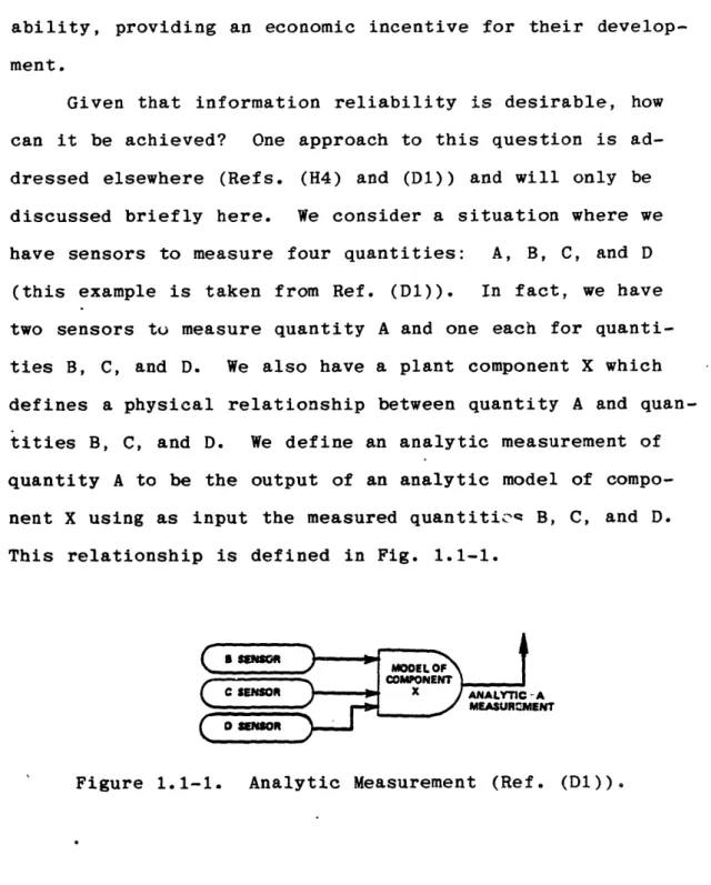
compo-nent X using as input the measured quantitioe B, C, and D. This relationship is defined in Fig. 1.1-1.

-A

IENT

Before pursuing this example any further, we pause here

to define a decision/estimator (D/E). The inputs to a D/E.

consist of all measurements of a quantity of interest; these

measurements can be both direct sensor measurements or

anal-ytic measurements. The D/E performs two functions:

1.) detection and isolation of inconsistencies in

the multiple measurements for a given

varia-ble; and,

2.) uses remaining consistent input measurements

to obtain a single estimate of the given

variable.

Figure 1.1-2 shows the symbol used to represent a D/E. The

D/E shown in this figure has three input measurements and

one output corresponding to the estimated value of the

meas-urement. The arrow emerging from the side of the D/E

indi-cates the detection and isolation of inconsistencies in the

input measurements.

Figure 1.1-2. Decision Estimator (Ref. (D1)).

Returning to our example, we use the two direct sensor

measurements of quantity A together with the analytic

meas-urement of A as inputs to a D/E, as shown in Fig. 1.1-3.

of the value of the measured quantity A. There are several

comments regarding Fig. 1.1-3:

Figure 1.1-3. Generation of a Best Estimate Value of Quantity A (Ref. (D1)).

1.) The inputs to the model of component X could consist of validated estimates from other

D/Es, as well as direct sensor measurements;

2.) The method usually does not require

installa-tion of addiinstalla-tional sensors in power plants,

particularly in major plant systems; and,

3.) The methodology has fault detection capabil-ity (Ref. (D1)).

In order to generate an analytic measurement, we need a

model of plant component X. This model is required to run in real time, or faster, in parallel with all other plant

computer tasks. The model should be derived from physical

laws applying to the component in question. A physically

be applied to a wide range of operating conditions while

empirical models are generally limited to the narrow range

of operating conditions for which they are obtained. Both

the DASS and SPDS need plant component models in order to

generate parameters relevant to plant safety. For this application, the models are also required to run in real

time and should be physically derived. Finally, if we ob-tain much faster than real time computing capability, then

these models can be used in a predictive manner to aid

oper-ations personnel in making decisions concerning alternate

control actions to be initiated during off-normal plant

transients.

In summary, the judicious application of physically derived, accurate, faster than real time computer models of

major plant components can result in systems that improve

the reliability of information displayed to plant operators

or used in closed loop control, improve plant availability,

and provide the operator with predictive capability.

1.2 RESEARCH OBJECTIVES

The main objectives of this work are to develop and validate an analytic model of a vertical U-tube natural

circulation steam generator, which is a major component in

many pressurized water reactor (PWR) plants (the other type

of steam generator in PWR plants is the once-through steam

generator). The model should satisfy the criteria set down

1.) Real time operation of the model; and,

2.) Model development based on the application of

fundamental physical laws rather than an

empirically derived model.

Model development is accomplished by the application of the laws of conservation of mass, momentum, and energy to

control volumes constituting the steam generator. The

con-trol volumes selected and the physical assumptions used in

these control volumes are based on considerations such as

geometric configuration, the physics occuring within the

various steam generator regions, and constraints arising

from numerical solution techniques.

The task of model validation is the comparison of the

computer model results with experimental data and/or results

generated by other computer codes that have been well

vali-dated. This step ensures model fidelity and helps determine

the limits of model applicability. A thoroughly validated

model can be used with confidence in an operational safety system.

An additional dividend resulting from the development

of a fast, physically based steam generator model is that

such a model bridges the gap between simplified boiler-pot

models and the more complex, computer-time-consuming codes

such as RETRAN (Ref. (M8)), URSULA2 (Ref. (K2)), and

1.3 PREVIOUS WORK

Little literature exists relevant to the real time

modeling of steam generators. However, there is a fair

amount of information available dealing with steam generator modeling in general. A good literature survey of transient

modeling of nuclear steam generators is given in Ref. (L2),

so a literature review will not be given here.

Much of the recent work in steam generator modeling

involves detailed, three-dimensional, two-fluid representa-tions of the boiling side of the steam generator (Refs.

(K2), (M7), (S2), and (I2)). The computer models derived in

the references given above are used to generate detailed flow conditions for either steady state or transient cases.

The detail is obtained only by spending large amounts of

computing time as shown in Table 1.3-1. Note that the

geo-metric detail of these models ranges from 4900 cells to

about 500 cells, while the model developed in this work has

4 cells. Less detailed computer models are developed in

Refs. (V1), (H5), and (L3); these models use

one-dimen-sional, slip-flow (not two-fluid) representations of the

boiling side of the steam generator. The TRANSG code (Ref.

(L3)) when used to model a once-through steam generator with a fixed time step size of 0.05 seconds requires 16 seconds

of computer time to simulate 10 seconds of real time on an

Amdahl 470/V6 computer system. (Computation time results

quoted here vary with the size o the problem being solved -for the TRANSG problem mentioned above this is 20 cells -for

00

o00

0

oJ

0

0

) OD UD >D

0

..

,

,

.w

iL

C

.u

C.

A

C.)

)

V C)

o

.)

.

r

1C

4.4

C

~0E

o

~

~

~

~

~

O

4O

0

)

00

E-

both the primary and secondary sides.)

Although none of the

works cited here deal with real time modeling of steam

gen-erators, they are useful guides in developing real time

computer models since they provide insightful information concerning steam generator dynamics and modeling.

The most relevant work with respect to real time model-ing is a thesis by Clarke (Ref. (C2)). In this work Clarke

uses a lumped parameter approach in the treatment of the secondary regions of the steam generator. The model is

simple, but it retains the essential physical features ne-cessary to reproduce gross steam generator dynamics.

1.4 ORGANIZATION OF REPORT

Chapter 2 is an overview of the steam generator model

developed in this work. Chapter 3 provides detailed

infor-mation regarding the development of the secondary side

mod-el. The primary side model, along with the heat transfer

model, is developed in Chapter 4. The numerical solution

scheme, including a discussion of stability concerns, is

given in Chapter 5. Model validation is discussed in

Chap-ter 6 and Appendix H. Conclusions and recommendations, as well as a summary, are given in Chapter 7. Appendices I and

J contain a description and listing of the computer

pro-gram. An interesting attempt to use boundary conditions for

transient calculations other than those given in the main

text is presented in Appendix G. The remaining appendices

Chapter 2

STEAM GENERATOR MODEL: OVERVIEW

2.1 DESCRIPTION OF STEAM GENERATOR

Heat generated by the nuclear chain reaction in the core of a pressurized water reactor is removed by the

pri-mary coolant and is transferred to the secondary coolant via

the steam generators. This heat transfer results in the

production of secondary steam which is then used to drive a

turbine-generator set.

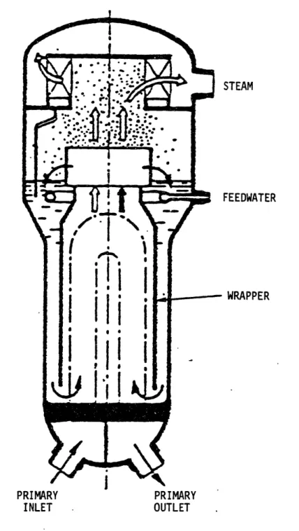
A representative U-tube steam generator (UTSG) is shown

in Fig. 2.1-1. The unit consists of two interacting fluid

systems: the hot primary fluid system and the colder

secon-dary fluid system.

The primary and secondary sides are

linked by heat transfer

through the tube walls.

The primary

fluid system consists of the hot reactor coolant on the tube

side of the tube bundle, as well as the primary coolant

contained in the inlet and outlet plena located at the

bot-tom of the steam generator. Hot reactor water enters the

steam generator through the primary inlet nozzle. It then

flows inside the U-tubes, first upward and then downward,

where it transfers heat to the secondary fluid. The coolant

then leaves the outlet plenum through the outlet nozzle.

STEAM

FEEDWATER

WRAPPER

PRIMARY PRIMARY

INLET . OUTLET

the tube bundle and riser, and the outer (downflow) egion

consisting of the downcomer and feedwater mixing region.

Subcooled feedwater is introduced into the steam generator

via the feedwater nozzle and is distributed throughout the feedwater mixing region by the feedwater ring. There it

mixes with the recirculating saturated liquid returning from

the steam separation devices. The resulting subcooled

li-quid flows downward through the annular downcomer region

formed by the rapper and the steam generator outer shell.

At the bottom of the downcomer, the water is turned and

flows upward through the shell side of the tube bundle

re-gion, where it is heated to saturation and boils. The

sec-ondary fluid exits the tube bundle region as a saturated

two-phase mixture and flows upward through the riser into

the steam separating equipment. Steam separation is

achieved by using a combination of centrifugal steam

sepa-rators, for bulk liquid-vapor separation, and chevron type

steam dryers, for the removal of any residual moisture. The

relatively dry steam leaves through the steam outlet nozzle

at the top of the steam generator, while the saturated water

is directed downward to mix with the entering feedwater.

The secondary fluid path just described constitutes a

natural circulation loop. The driving head for this

recir-culation flow is provided by the density difference between

driving head is counterbalanced by the various pressure

losses in the loop, such as frictional losses in the tube bundle and the losses within the steam separators.

Load changes in UTSG units are accompanied by changes

in the secondary pressure, primary coolant inlet tempera-ture, feedwater flowrate, and feedwater temperature. Since

the steam generator heat transfer rate is essentially

pro-portional to the difference between the primary coolant

temperature and the secondary saturation temperature, and

since the saturation temperature is a function of saturation pressure, a change in secondary pressure results in a change

in the primary-to-secondary heat transfer rate. For

exam-ple, a load demand increase may be satisfied by increasing

both the primary inlet temperature and feedwater flowrate, along with a decrease in secondary pressure.

2.2 MODEL REGIONS

For the purposes of developing a model of the steam

generator, it is necessary to divide both the primary and

secondary sides into several regions. As a matter of prac-ticality, these model regions correspond to actual physical

regions of the steam generator. This allows us to specify

with greater accuracy the different physical processes

oc-curring within each region. For instance, in the downcomer

we are primarily interested in the flow of a subcooled

liq-uid, while in the tube bundle portion of the secondary side

we are interested in describing a two-phase flow with heat

addition. These are two essentially different physical

processes requiring different modeling techniques; hence, we

require two separate model regions. However, one must avoid

the temptation to use too many model regions since this can

result in a large and computationally costly model, which is

contrary to the goals of this work.

The steam generator model developed in this work has

four model regions on the secondary side and three model

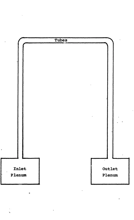
regions on the primary side. The primary side regions

con-sist of the inlet plenum, the fluid volume within the tubes

of the tube bundle, and the outlet plenum (Fig. 2.2-1). The

four secondary regions are: the tube bundle region; the

riser region; and, the steam dome-downcomer region, which is

divided into a saturated volume and a subcooled volume

(Fig. 2.2-2). The saturated nd subcooled volumes have a

movable interface; thus these volumes are not constant.

However, the sum of their volumes is constant and equal to

the total volume of the steam dome-downcomer region. There

are three constraints imposed on the model of the regions

contained within the steam dome-downcomer. The first is

that the interface between the saturated and subcooled

re-gions can never be above the level of the feedwater ring.

This constraint is motivated by physical considerations,

since one would not expect to find subcooled liquid above

Tubes

Inlet

Plenum

Outlet

Plenum

Figure 2.2-1

Primary Side Regions

r

- I- - - - --L

. . ,

IF

STEAM OUT RISER

-FI

0

u,

--subcooled water downward. The second constraint is that

there is always a minimum amount of saturated liquid present

in the saturated region. The final constraint is that the

feedwater is always added to the subcooled region, although

this is not always true during steam generator off-normal

operation. The last two constraints are discussed at length

in Section 3.3. The steam separators, although not

expli-citly treated, are accounted for by assigning a loss

coeffi-cient for pressure drop calculations and by assuming that

they always accomplish complete phase separation.

2.3 AUXILIARY MODELS

In order to simulate the effects of control actions

initiated in the main steam and feedwater systems on steam

generator performance, we have included simple models of

these systems in the overall steam generator model as an

alternative to providing the time-dependent steam and

feed-water flows as input. These models are fully developed in

Section 3.6; here we simply describe the systems and their

operation.

A schematic of a typical main steam system is shown in

Fig. 2.3-1. The main steam line extends from the steam

generator steam outlet nozzle to the high pressure turbine

main stop and control valve. The main steam line is also

provided with a main steam isolation valve (MSIV), which

o

r

Figure 2.3-1

0

0

I-

_LCf

Lad

0

E-4,>

Typical

Main Steam System

L

0

0

0

O

serves to isolate each steam generator in the event of a

main steam line break and thereby limits the steam generator

inventory loss. The MSIV also closes on a low steam genera-tor pressure signal in order to prevent overcooling of the

primary system fluid. There are also a number of steam

relief systems associated with the main steam line. These

are the steam dump, turbine bypass, and safety relief valve

systems. The steam dump system vents to the atmosphere.

The turbine bypass system diverts steam directly to the

condensers and serves to limit steam pressure during

opera-tional transients. The bypass system is also used during

hot standby and shutdown cooling. Both the steam dump and

turbine bypass systems are used during load rejections in

order to limit the ensuing secondary pressure rise. This

action maintains the steam generator heat removal capability

and prevents excessive increases in primary system

tempera-tures. The safety relief valve system consists of a number

of pressure relief valves located upstream of the MSIV.

This is a passive system requiring no operator or control

system action since the valves are spring loaded and open if

the steam pressure is greater than the spring force. The

steam relief capacity of this system is generally 5 to 6 per

cent larger than the main steam flowrate at full power

conditions.

The feedwater system consists of the feedwater heaters,

feedwater pumps and feedwater regulating valves. Modeling

of this system in itself is a difficult task and is not

at-tempted in this work. The feedwater temperature, in

partic-ular, is a required input to the steam generator model since determining this quantity would require a model of the

feed-water train, including extraction steam, which is beyond the

scope of this work.

A simple model of the feedwater control system is

in-corporated into the overall steam generator model so that one can simulate controller effects on feedwater flowrate.

The feedwater flow controller is a three-element controller

that monitors steam flowrate, feedwater flowrate, and steam

generator water level. The controlled quantity is the steam

generator water level, and its control is accomplished by

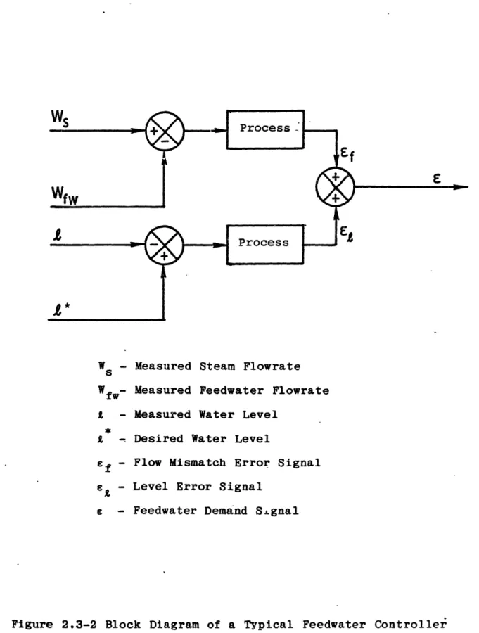
regulating the feedwater flowrate. Figure 2.3-2 is a block

diagram of the controller. The measured steam and feedwater

flowrates are -compared and processed to provide a flow mis-match error signal. The measured water level is compared to

the desired water level, and the difference between them is

processed to provide a level error signal. The flow

mis-match and level error signals are then combined to produce a

feedwater flowrate demand signal that either increases or

decreases the feedwater flowrate.

In Chapters 3 and 4 we develop in detail the steam

generator primary and secondary side models, as well as the

a

*

Ef

E

Ws

-

Measured Steam Flowrate

Wfw- Measured Feedwater Flowrate

£

X - Desired Water Level

£f - Flow Mismatch Error Signal

eG - Level Error Signal

£ -

Feedwater

Demand Sgnal

Figure 2.3-2 Block Diagram of a Typical Feedwater Controller

Chapter 3

SECONDARY SIDE MODEL

The most challenging part of the steam generator from a

modeling point of view is the secondary side. The modeling

difficulties are due to the following:

1.) Strong coupling between all regions of the secondary side;

2.) Natural recirculation flow;

3.) Both two-phase

and single

phase

conditions

exist; and,

4.) Geometry.

The following sections describe in detail the development of

the secondary side model.

3.1 TUBE BUNDLE REGION

3.1.1 Mass and Energy Equations

As described in Chapter 2, the recirculating secondary

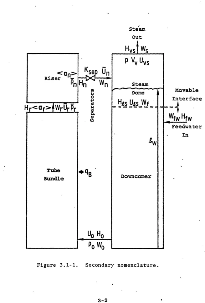
fluid is heated and boils in the tube bundle region. A

block diagram indicating the secondary side regions and the variables of interest is shown in Fig. 3.1-1 (see

Nomencla-ture for variable identification). As discussed in Appendix

B, we are using a model in which all system fluid properties are evaluated at a single, time-dependent reference pres-sure. It should be noted that the flow pattern and heat

Steam

Out

Hvs Ws

Steam

HS

US

Wf

£w

Downcomer

Movable

Interface

Feedwater

In

Figure

3.1-1.

Secondary nomenclature.

<

an

Riser

Hr<ar>i#wrUr Pr

Ksep Un

Q n

n

k

. s

Tube

Bundle

I'' I

- - --'J ---

Since the primary fluid is cooled during its journey through

the tubes, the heat transfer rate varies along the length of

the tubes. This results in a "hot side" and a "cold side"

of the steam generator, which correspond to the upflow and

downflow portions of the tubeside fluid. This spatially

non-uniform heat transfer causes the secondary side flow

pattern in the tube bundle to be non-uniform. In addition,

there is a flow redistribution within the crossflow region

of the tube bundle. Thus, although we use a one-dimensional

treatment for the fluid on the shell-side of the tube

bundle, the flow conditions are truly three-dimensional.

Using the mass and energy equations developed in

Appendix B and neglecting heat transfer to the steam

genera-tor structural material, we obtain:

dM

dTB = W - Wr (3.1-1)

and,

dtTB W H WrHr+ q (3.1-2)

Solving Eq. (3.1-1) for Wr and substituting the result

into Eq. (3.1-2) yields,

dETB

H

MB

= W(H-

H )

+

q

(3.1-3)

Equation (3.1-3) is in a form which is independent of

en-thalpy reference point (see Appendix B, Section 4).

3.1.2 Integration by Profiles

In order to solve Eq. (3.1-3) we need to determine

ETB and MTB. Both of these quantities are integrals of

either the density or the product of density and internal

energy over the tube bundle volume. Since we are using a

one-dimensional approach we really need only integrate over

the length of the tube bundle taking into account, of

course, flow area changes. Thus, the problem is reduced to

finding, or making an approximation regarding, the axial

profiles of the fluid density and internal energy in the

'tube bundle. Determining the transient axial profiles of

these quantities is a time consuming task, and since we are

interested in computational speed we choose to make some

approximations in obtaining these profiles. One condition

that seems appropriate for these profiles to satisfy is that

they reduce to the correct steady state profiles. In

addi-tion, we are interested in transients which are

signifi-cantly longer in time span than the fluid transport time

through the tube bundle (see Table 3.1-1 for representative transport times). Therefore, it is reasonable to assume

that each transient profile adjusts slowly and is similar to

some steady state profile. So now the question is: What

Table 3.1-1

Representative Fluid Transport Times

3.1.3 Detailed Profiles

Before we can answer this question we must take a

closer look at the tube bundle region and the physical pro-cesses occuring there. This is best accomplished by

per-forming a detailed one-dimensional steady state

thermal-hydraulic analysis of the tube bundle region. In this

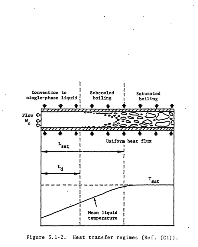
region we can identify three flow and heat transfer regimes

(see Fig. 3.1-2):

1.) Heat transfer by forced convection to

a subcor,led liquid;

2.) Heat transfer via subcooled nucleate

boiling; and,

3.) Heat transfer by saturated nucleate

boiling.

pro-Convection to

single-phase liquid

Flow 0

Subcooled

boiling

Saturated

tP

tP

_4

4

--

4 4 4 4 4

_

4

--I

Uniform heat flux

! I I I I I Mean liquid I I temperature I 1 I

Figure 3.1-2. Heat transfer regimes (Ref. (C1)).

$+

+

i r +I

+

,77 77

"7 77 7 77

-- -- I-1 1 , 1 0

0 ( 5

r3

The approach taken here is to develop a detailed com-puter model subject to the following:

1.) Uniform axial heat flux;

2.) Single pressure for property evaluation;

3.) Onset of subcooled boiling determined

by the empirical bubble departure

criterion of Saha and Zuber (Ref. (L1));

4.) Subcooled and saturated flow quality

distributions provided by a

profile-fit model (Ref. (L1)); and

5.) Vapor volume fraction-flow quality

relationship described by the drift

flux model (Appendices A and C).

In this detailed model we use steady state heat balances to

determine the fluid axial enthalpy distribution. Thus, the

axial position at which the fluid bulk temperature reaches

the saturation temperature is given by,

W(H s- HIN)

L (3.1-4)

LSAT ATq (3.1-4)

However, subcooled boiling occurs before the bulk of the fluid is at saturation. The subcooled boiling region is

further divided into two regimes. In the first region vapor

is generated, but the vapor bubbles collapse immediately

bubbles do not collapse immediately after they detach from

the wall. This second region starts at the so-called bubble

departure point and is the more important of the two

regions. We will, therefore, neglect the first region and

assume that the onset of subcooled boiling is coincident

with the bubble departure point. The Saha-Zuber criterion

for the bubble departure point is:

H s (H)d - (0.0022) Pe q Pe < 70,000

Hs - (H ) 154 " Pe > 70,000

where

G DhCP

Pe

-

Peclet Number

=

and (HL)d fluid bulk enthalpy at the bubble departure

point.

So the axial position at which subcooled boiling occurs is

W ((H )d

HIN)

Ld = qHT (3.1-5)

Upstream of Ld is very little vapor, between Ld and LSAT the bulk fluid temperature is less than the prevailing

satura-tion temperature but there is a net producsatura-tion of vapor, and

liquid and vapor.

Thus, the density and internal

energy

distributions are

U = U

<a>

Pvs

+ (1

-

<>)P

U

(>

U

=

[ <>PvSUVs + (1 - <>)PtSUIs

_/

We still

need to determine the distribution

of <a). By

using the drift

flux model we can obtain

< a> once we know

x.

As mentioned earlier,

we are using a profile-fit

model

to predict the flow quality distribution.

In the

profile-fit model we assume that the mean liquid enthalpy, H, is

the following function of the enthalpy, H',

(H s - Hl)

its

Id

but,

H' = H(1 - x) + Hvsx

so,

(H - Hs) + [Hs - (H )d]

X

tHvs

At this point we have completely specified and solved

the problem. All that remains is a discussion of how this

scheme is implemented on the computer.1 Simply stated, the

tube bundle is divided into a number of nodes and the

various parameters of interest (H', x, <>, p and U) are

then calculated. The nodalization scheme is determined by

Ld and LSAT . The length extending from the tube bundle

inlet to Ld is divided into five nodes, as is the distance

between Ld and LSAT. The remaining length from LSAT to the tube bundle outlet is divided into ten nodes.

The required inputs for this calculation are the power,

system pressure, inlet flowrate, inlet density, and inlet

internal energy. The system conditions used for the

calcu-lations presented here are representative of current nuclear

U-tube steam generators. These parameters are listed in

Table 3.1-2.

1 This is a preliminary calculation for verification pur-poses only. This scheme is not used in the final steam

generator model.

Table 3.1-2

Inputs for Detailed Profile Calculations

Table 3.1-3 lists the fractional lengths at which

bubble departure is calculated, and the fractional lengths at which bulk saturation conditions occur. The results

clearly indicate that subcooled boiling, as predicted by the

bubble departure criterion, plays a significant role at all

power levels. That is, anywhere from 9 percent to 12

percent of the tube bundle length is in subcooled boiling.

Thus, flow quality and vapor volume fraction profiles start

Table 3.1-3

Results of Detailed Profile Calculations Bubble Departure and Saturation Lengths

3.1.4 Approximate Profiles

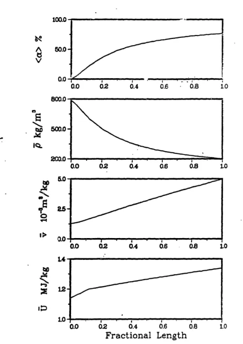
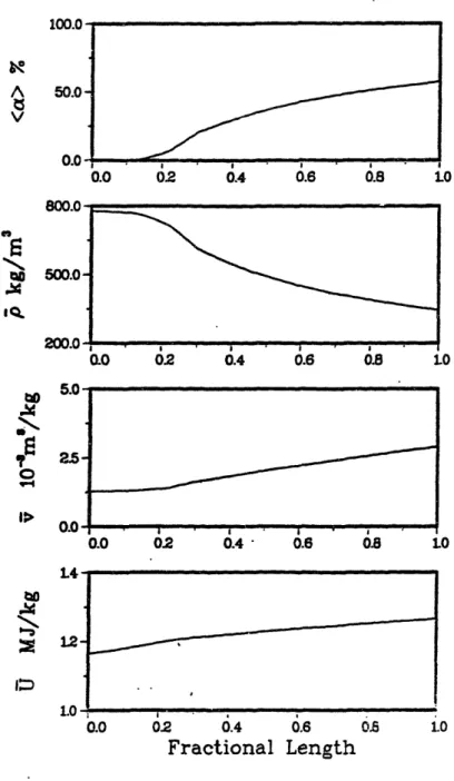
Figures 3.1-3 through 3.1-5 are plots of <a>, p, v

(v = l/p) and U versus fractional length for power levels of 100%, 40%, and 5 of the nominal power (817 MWt). The

plots of interest are those of v and U. The figures show

that these quantities are nearly linear functions of

posi-tion. This observation, together with the fact that

sub-cooled boiling starts very near the tube bundle inlet, leads

us to the assumptions that the density varies inversely with

axial position, while the internal energy varies in direct

proportion to the axial position.

Percent

Ld/LTot

LSAT/LTot

Power

40

0.0993

0.2248

50.0-0. .2 I .6- - '. 1 0.0 02 0.4 0.6 0.8 0.0 02 0.4 0.6 0. I I I 0.0 02 0.4 0.6

Fractional Length

Figure 3.1-3.

10C V 0.0 800.0 500.0 XII,.

Q

. S

I;

100 5 0.0-ODM OW.U -

500.0-

0f

io

Fractional Length

Figure 3.1-4.

Profiles at 40 per cent power.

v

as

0

~

~

~

100.0 0 A V 80O-. 500.0-LO 02 · 0.4 ' 0.6

0.

.

I

.

0.4I 0

0

.

25

CLO s-o oz 02 cx~~ U i t'~e O.i 0.8 i

LU -- I I I 02 0.4 0.6

Fractional Length

Figure 3.1-5. Profiles at 5 per cent power.

I

0

-4

12-~I

It might seem at first glance that these assumptions are not self-consistent. However, we will show that they

are indeed consistent in saturated two-phase regions, and

that assuming one profile directly implies the other.

Starting with the density being inversely proportional to

axial position we have,

1 1 = Az + B (3.1-6) p But U = + P and <a> =

Pts - Pvs

_-

_vsvs

-

p/sUQS)

pis

Pvs

into the previous expression

+ B) - 1

= Cz + D

s - Pvs

Substituting this result and Eq. (3.1-6) into Eq. (3.1-v),

U

or

(3.1-7)

U Ez + F (3.1-8)

Thereby demonstrating that if p is inversely proportional to

axial position, then U is directly proportional to axial

position in saturated two-phase regions.

3.1.5 Approximation Errors

In order to gain insight into the magnitude of the error generated by extending linear profiles to other

re-gions, we can perform some straightforward calculations.

Equation (3.1-6) can be written as

1

=

[i

_

I]

+1

P Pr T0 LTB 0o

Substituting this expression into the definition of MTB

yields

VB

VTBOP

TBB

I

dV

TB

OPr)

n

(3.1-9)

o

PO -

r

Pr

Equation (3.1-8) can be written as,