Vertical distribution of the void fraction, using X-ray attenuation measurements, for different flow regimes in a horizontal pipe

HAL Id: cea-02439449

https://hal-cea.archives-ouvertes.fr/cea-02439449

HAL is a multi-disciplinary open access

archive for the deposit and dissemination of sci-entific research documents, whether they are pub-lished or not. The documents may come from teaching and research institutions in France or abroad, or from public or private research centers.

L’archive ouverte pluridisciplinaire HAL, est destinée au dépôt et à la diffusion de documents scientifiques de niveau recherche, publiés ou non, émanant des établissements d’enseignement et de recherche français ou étrangers, des laboratoires publics ou privés.

attenuation measurements, for different flow regimes in

a horizontal pipe

L. Rossi, R. de Fayard, S. Kassab

To cite this version:

L. Rossi, R. de Fayard, S. Kassab. Vertical distribution of the void fraction, using X-ray attenuation measurements, for different flow regimes in a horizontal pipe. NUTHOS 11th - International Topical Meeting on Nuclear Thermal Hydraulics, Operation and Safety, Oct 2016, Gyeongju, South Korea. �cea-02439449�

1/12

VERTICAL DISTRIBUTION OF THE VOID FRACTION, USING X‐RAY ATTENUATION 

MEASUREMENTS, FOR DIFFERENT FLOW REGIMES IN A HORIZONTAL PIPE 

L. Rossi, R. De Fayard, S. Kassab

CEA, Paris-Saclay University, Den-STMF F-91191, Gif-sur-Yvette, France Name of Organization

lionel.rossi@cea.fr

ABSTRACT

METERO is an experimental facility built by the French Atomic Energy Commission (CEA) aimed at studying adiabatic air-water flows in horizontal pipes. The physical insight and the experimental data provided by METERO experiments support the validation of MCFD (NEPTUNE CFD) and System (CATHARE-3) codes as a part of the NEPTUNE project developed jointly by EDF, CEA, AREVA NP and IRSN. [Bottin et al International Journal of Multiphase Flow 60 (2014) 161–179] have proposed a flow map of the different regimes encountered in the METERO experiments, i.e. stratified flows, slug flows, plug flows, stratified dispersed bubbly flows and dispersed bubbly flows. Following this work, we investigate the vertical distribution of void fraction integrated horizontally using X-ray attenuation measurements.

After a description of the experiments and the measurements’ method, we discuss the evolution of the vertical distribution of the void fraction in horizontal pipes and derived statistics such as the ratio of the air and water phase velocities. Different flow regimes and their transitions (e.g. slug, plug, and bubbly regimes) are explored by varying the water and air superficial velocities.

KEYWORDS

FLOW REGIME, X-RAY MEASUREMENTS, VOID FRACTION, HORIZONTAL PIPE

1. INTRODUCTION

Vertical bubbly flows have been extensively studied, e.g. [1, 2, 3, 4, 5] whilst less literature can be found about multiphase flows in horizontal pipes, e.g. [6, 7, 8]. The dynamic of multiphase flows in horizontal pipes differs from the one observed in vertical pipes due to the fact that gravity is perpendicular to the mean flow and not parallel. The buoyancy forces tend to have bubbles moving up. They then support the accumulation of air in the upper part of the pipe which favours the coalescence of bubbles. The turbulence is amenable to disperse bubbles and to provoke the coalescence and break up of bubbles. The competition between buoyancy and turbulent forces in horizontal pipes results in different flow regimes from stratified flows to dispersed bubbly flows [8].

The pipes’ lengths of nuclear power plant are generally (primary circuit) about ten times their diameters. Potential multiphase flows in such short pipes would not reach a fully developed stage. The knowledge, modelling and simulation of transient horizontal two-phase flows are therefore important for safety studies of nuclear power plant. Existing literature and experimental data need to be completed by experiments in relatively short pipes.

METERO is an experimental facility built by the French Atomic Energy Commission (CEA) aimed at studying adiabatic air-water flows in horizontal pipes. The physical insight and the experimental data provided by METERO experiments support the validation of MCFD and CATHARE-3 codes as a part of the NEPTUNE project developed jointly by EDF, CEA, AREVA NP and IRSN. The main purpose of

2/12

METERO experiments is to help improving the accuracy of numerical tools by providing new physical insights and data for validation.

Measurements using X-ray attenuation are amenable to indicate the structures of multiphase flows where the phases’ attenuations are different, e.g. [9, 10, 11, 12, 13]. The void fraction within air-water flows can then be measured using X-ray attenuation. Using such measurements, the present manuscript focuses on the vertical distribution of the void fraction and deduces physical quantities such as air and water phase velocities.

The manuscript is articulated as follows. First the experimental rig, the measurement methods and the flows’ parameters investigated are introduced. Then results obtained from measurements performed over different flow regimes and at different longitudinal positions (10.4D, 20.6D and 41.3D) are presented and discussed.

2. EXPERIMENTAL

DESCRIPTION

2.1. Experimental setup

METERO is an experimental rig dedicated to the study of turbulent mixing of air and water in horizontal flows. Extensive descriptions of METERO can be found in [14, 15, 8].

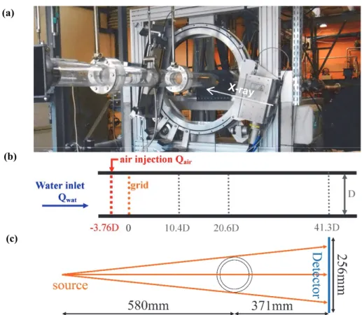
The pipe is of circular shape and is assembled from different modules made in Perspex. The Perspex walls are 10mm thick. The inside diameter of the pipe, i.e. the diameter of the flow cross section, is D=100mm. D is chosen as the reference length scale. Dimensionless length scales, according to D, are noted with a superscript star, e.g. ∗ ⁄ . Fig. 1a is a photo of METERO’s test section.

Figure 1: (a) photo of the test section with the encapsulated X-ray source and of the X-ray detector mounted on a rotating device; (b) schematic of the test section with relevant longitudinal positions; (c) schema of the X-ray source and the angular distribution of X-ray beams crossing the test section.

(a)

(b)

3/12

The water flow rate within the pipe section is noted Qwat. It is measured using either MHD

(electromagnetic) or Coriolis flow meters according to the flow intensity. At the entrance of the test section, the air is regularly injected in space over 37 nozzles with inside diameters of 1.2mm. The air flow rate is measured using mass flow meters and is noted Qair. 3.76D downstream the injection, a

turbulent grid (mesh of 2.71mm with wires of 0.71mm diameter) mixes the flow and breaks air bubbles. The longitudinal (or flow) direction along the pipe is noted x and the vertical direction is noted y. The position of the grid is chosen as the x axis origin. The axis of the pipe is chosen as the origin of y. Fig. 1b illustrates these positions and notations. Downstream the test section, a water tank at atmospheric pressure is used to separate the air from the water. This black tank is visible on the right of figure Fig. 1a.

The X-ray beams are emitted from a localised source at 160kV and 18.75mA. It is collimated so as to illuminate a plane perpendicular to the axis of the test section. Fig. 1 shows a photo of the encapsulated source and the detector along with a schematic of the emitted X-ray beams. The X-ray intensity is recorded by the Hamamatsu C9750-10TC detector. This linear detector possesses 1280 pixels of 0.2mm with a 12bits depth. The dark image of the detector (signal with X-ray turned off) is removed from the recorded signal. The resulting signal level is proportional to the amount of X-ray received by the detector.1 The X-ray source and detector are mounted on a rotating system so as to vary the angles of the measurements.

2.2. Void fraction measurements using X-ray attenuation

Void fraction measurements using X-ray attenuation relies on the difference of attenuation of the incident X-ray beam between the gas and liquid phases.

The attenuation of a X-ray along a material line is modelled as:

dI μI dx (1)

This leads to Beer-Lambert law for X-ray attenuation for a given material

(2) is the initial intensity of the beam, is the intensity of the X-ray beam transmitted through the

material, [in m-1] is the linear attenuation of the material and x [in m] is the thickness of the material crossed by the X-ray beam.

Successive attenuations through different materials lead to successive multiplications by where is the attenuation coefficient of the ith _{material crossed. The X-ray intensity transmitted through}

successive elements is:

∏ (3)

In METERO experiments, the X-ray successively crosses the air, the Perspex, the flow, the Perspex and the air before reaching the X-ray detector. This is illustrated in Fig. 2. The attenuation of the X-ray beam can then be written as:

I I e e (4)

where μ x is the attenuation from the air outside the test section, μ x is the attenuation due to the Perspex, μ x and μ x are respectively the attenuation due to the water and the air within the test section.

The void fraction along the X-ray path, inside the flow section, is noted α and is defined by:

α (5)

4/12

l x x is the length of the path of the X-ray beam within the flow. The combination of equations (4) and (5) leads to:

ln Aα B (6)

The measurement of the void fraction using X-ray attenuation relies on the determination of the constants A and B through calibration. In practice, A and B are estimated using measurements with the pipe full of air and water.2

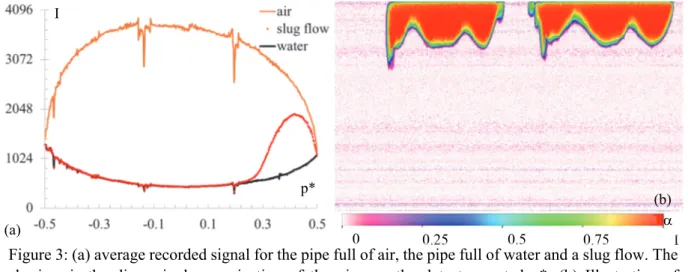
Fig. 3a illustrates the temporal average of the signals obtained for the pipe full of air, full of water and for a slug flow. This permits to measure the void fraction along the path of the X-ray beam during each exposition of the detector. For this slug flow, Fig. 3b gives a pictorial illustration of such temporal measurements during 2.816s. Each column of the picture represents one measure of the 1D X-ray sensor and the picture is made of 1280 columns.

The accuracy of void fraction measurements is checked by varying the water depth within the pipe while the flow is at rest. The measured void fraction can then be estimated from simplified geometrical

2  _{This  linear  relation  between    and  ln(I}

x/I0)  supposes  that  the  effects  of  the  hardening  of  the  X‐ray  beams  spectrum are negligible. The validity of this hypothesis is confirmed later. 

Figure 2: schematic of an X-ray beam crossing a bubbly flow within the test section

0 0.25 0.5 0.75 1

Figure 3: (a) average recorded signal for the pipe full of air, the pipe full of water and a slug flow. The abscissa is the dimensionless projection of the pipe on the detector, noted p*. (b) Illustration of temporal void fraction measurements (the color scale shows α) for a slug flow and a duration of 2.816s. The columns of the picture correspond to 1280 consecutive 1D measurements. For (a) and (b) the X-ray sensor is vertical, which corresponds to the position referred as 0°.

(b) (a)

I

p*

5/12

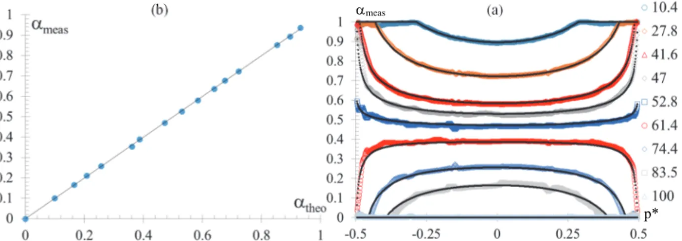
Fig. 4a illustrates the comparison between measured and theoretical void fraction. The average of the root mean square of the differences between measured and theoretical values is about 0.013. This result indicates the accuracy of the void fraction measurements performed.

Fig. 4b gives the measured void fraction versus the theoretical values along the median vertical axis of the pipe. There is a good agreement between these values which follows the straight line αmeas=αtheo.

Moreover, the linearity of this result shows that the relation between ln(Ix/I0) and  can well be

considered as linear with negligible effects of the hardening of the X-ray beams spectrum in these experiments. This is thanks to the increase in voltage, i.e. X-ray energy, since previous works at 40kV [16] demonstrated such a hardening effect.

To build the vertical distribution of the void fraction within the pipe, several angular positions of the source-detector pair are needed. Indeed, the void fraction is measured along the path of the X-ray beams and these beams are not all parallel to the horizontal. To ensure deviations from the horizontal smaller than 0.5mm, between the two extremities of the flow cross section along the X-ray path, seven angular positions are needed. These positions are -3.5°, -2.25°, -1.1°, 0°, 1.1°, 2.25° and 3.5°. The vertical distribution of the void fraction is then built from these seven measurements by selecting the results minimalizing the deviation from the horizontal. It can be indicated that, with this set of angles, the mean Figure 4: void fraction measurements for different water levels within the pipe. (a) void fraction measured, noted meas, versus the projection of the pipe on the detector in abscissa, noted p*. The

legend indicates the water level in mm. The black dots correspond to theoretical estimations on a simplified geometry. (b) Measured void fraction, αmeas, versus theoretical void fraction, αtheo, along the

median vertical axis of the pipe.

(a) (b)

p* meas



Figure 5: estimation of the deviation of the X-ray beams from the horizontal (in mm) versus measurement positions ∗.

6/12

deviation from horizontal is 0.24mm with a standard deviation of 0.14mm. This discretisation over seven angles sounds sufficient as it is about the pixel resolution of the detector and it is smaller than the targeted 0.01D resolution of the measurement. The Fig. 5 gives the estimation of these deviation from the horizontal versus the measurements positions ∗. The seven minima observed, with deviations equals to zero, occur when the horizontal X-ray beams cross the corresponding measurement points.3

2.3. Experimental investigations

Experimental investigations are conducted at different axial positions downstream the grid (10.4D, 20.6D and 41.3D) and for different air and water flow rates. Experiments are performed at 18.05°C4 and atmospheric pressure.

METERO’s flow map according to the liquid and gas superficial velocities, respectively ⁄ and ⁄ where S is the flow cross section, has been established in [8] at about 40D downstream the grid. Fig. 6 gives the distribution of investigated flow parameters according to METERO’s flow map (at 40D) while table 1 gives corresponding numerical values. ReL refers to the liquid Reynolds number, ⁄ where  is the kinematic viscosity of the liquid.

Water Qwat [m3/h] 20 30 60 90 120 150 ReL 71 000 110 000 210 000 320 000 420 000 530 000 JL [m/s] 0.71 1.06 2.12 3.18 4.24 5.31 Air Qair [Nl/min] 10 20 30 40 50 70 90 120 150 200 250 300 JG [m/s] 0.023 0.045 0.068 0.091 0.11 0.16 0.20 0.27 0.34 0.45 0.57 0.68 Table 1: flow parameters varied in the experiments. Nl/min corresponds to the conversion of the measured mass flow rate in l/min for 0°C and 1atm.

3 _{The position of the minimum of deviation corresponding to the angle 0° is close to} ∗ _{0 but slightly different.}

This is due to the position of the pipe’s axis which is a slightly higher than the axis of the measurement device. 4  _{The variance of the recorded temperature is 0.76°C.} 

Figure 6: distribution of the experimental data according to METERO’s flow map [8] at 40D.

7/12

3. RESULTS

AND

DISCUSSION

To help comparing different flow cases an inlet void fraction, noted , is built as:

(7)

3.1. Vertical distribution of the horizontal void fraction at 41.3D

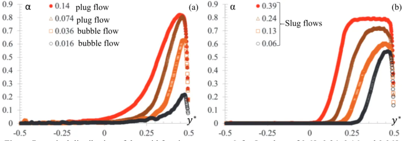
First the profile of vertical distributions of the void fraction, α, varying Qair for the Reynolds number

420 000 and 110 000 are given in Fig. 7 at 41.3D.

For ReL=420 000, the flows change from the bubble to the plug flow regime when increasing the air

flow rate. For all cases, the air accumulates in the upper part of the pipe. When increasing the air flow rate, the maxima of the void fraction increase toward a maximum value of about 0.8. It can be noted that for the plug flows the maximal value of α varies slightly and the main effect is an increase in the size of the plug and of the domain where the void fraction is significant, i.e. α≥0.02.

For ReL=110 000, the flow stays in the slug flow regime when increasing the air flow rate. The increasing of αQ leads to an increase of the maxima of α and an increase of the domain where the void

fraction is significant. The appearance of plateaus of increasing length for the maximal values is also an indication of the increase of the height of the slugs within the pipe.

Second, the profile of vertical distributions of the void fraction, α, varying Qwat for the JG values of 0.068

and 0.68 are given in Fig. 8 at 41.3D.

For JG=0.68 the flows change from slug to plug and bubble flow regimes when increasing the water

flow rate. As previously discussed, the slug flow cases present a plateau with an increase of the maxima values and of the domain of significant void fraction with the increase of αQ. Two new points are

interesting to note: i) the transition from slug flow to plug flow leads to an increase of the maximum value of α combined with the disappearance of the plateau; ii) the transition from plug to bubble flow regimes leads to a sharpening of the profile close to the maxima values of α and an increase of the domain where the void fraction is significant. This can be related to the dispersion of bubbles within the core of the flow by the turbulence [8].

For JG=0.068 the flows also change from slug to plug and bubble flow regimes when increasing the

water flow rate. This case complements the case JG=0.68 by focusing on cases with low values of αQ. It

can be noted that the bubble flow (which also corresponds to the highest Reynolds number) presents values of α larger than the other flow regimes in the core part of the flow, in particular for 0 ∗

0.3.

Figure 7: vertical distribution of the void fraction α versus ∗ _{for J}

G values of 0.68, 0.34, 0.16 and 0.068

m/s for (a) ReL 420 000 and (b) ReL 110 000. The corresponding values of αQ (0.14, 0.074, 0.036, 0.016

and 0.39, 0.24, 0.13, 0.06) are indicated in the symbols’ legend. x=41.3D.

(b) (a)

∗ ∗

α 

α

bubble flow Slug flows

plug flow bubble flow

8/12

3.2. Changes of α distribution with the development of the flow

3.2.1. Bubble flows

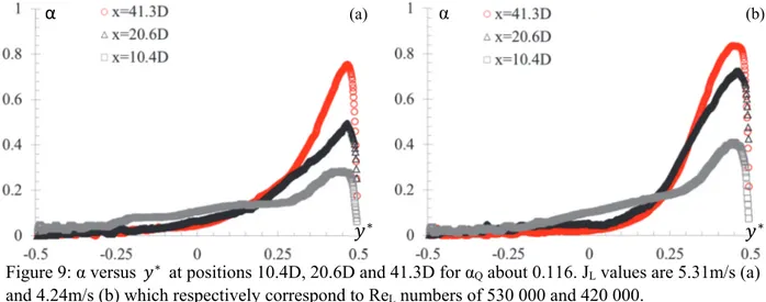
Fig. 9 shows the changes in the distribution of the void fraction with the longitudinal development of two bubble flows with αQ close to 0.116. With the longitudinal development of the flow, the void fraction

increases in the upper part of the pipe while it decreases in the bottom part for both cases. It is interesting to note that the results obtained for JL=4.24m/s and 5.31m/s looks similar for 41.3D and 20.6D

respectively.

Fig. 10a directly compares these two cases while 10b compares the same cases at positions 20.6D and 10.4D. These results are relatively close. This may support that the temporal integration of buoyancy effects has evolved similarly for both cases. Fig. 10c shows the comparison between JL=4.24m/s and 3.18m/s for αQ about 0.021 at positions 10.4D and 41.3D. Again the two results are close.

It is important to note that the time scales during which the buoyancy effects are integrated, i.e. the travelling time of the flow between the considered cross section and the inlet condictions for a given flow rate, are significantly different. The ratio of these durations are about 1.6 for Fig. 10a and Fig. 10b whilst it is about 3 for Fig. 10c. This highlights the impact of the turbulence on the void distribution and importance of nonlinear processes in the development of turbulent multiphase flows.

Figure 8: vertical distribution of the void fraction α versus ∗ _{for J}

L values of 0.71, 2.12, 3.18 and 5.31

m/s for (a) JG=0.68 and (b) JG=0.068. The corresponding values of αQ (0.49, 0.24, 0.18, 0.11 and 0.09,

0.031, 0.021, 0.013) are indicated in the symbols’ legend. x=41.3D.

(a) ∗ ∗

α 

α

Figure 9: α versus ∗ at positions 10.4D, 20.6D and 41.3D for αQ about 0.116. JL values are 5.31m/s (a)

and 4.24m/s (b) which respectively correspond to ReL numbers of 530 000 and 420 000.

(b) (a)

∗ ∗

9/12

3.2.2. Slug flows and complex transitions

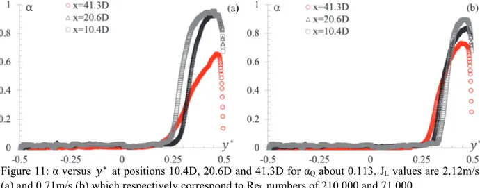
Fig. 11 shows the evolution of the profile of α versus ∗ at positions 10.4D, 20.6D and 41.3D for αQ=0.113, JL=2.12m/s and JL=0.71m/s. It can be noted that as opposed to the bubble flows cases, the

void fraction maxima decreases with the longitudinal development of the flow. Two different reasons can be highlighted: i) in the case of Fig. 11a the flow regime changes from position 10.4D to 41.3D. At 10.4D the flow looks like a bubble flow with a continuous plug (or foam) at the top. At 41.3D the flow has evolved toward a slug flow; ii) In the case of Fig. 11b, the flow regime is similar to a slug flow for the three positions. What is observed is an increase of the height of the slugs with a decrease of their frequency.

3.3. Void fraction in the flow cross-section versus αQ and relative phase velocities

The void fraction in the flow cross-section is estimated by integrating the horizontal void fraction over

∗_:

∗ ∗

.

. (8)

where S is the area of the flow cross-section, ∗ is the horizontal chord length at the height ∗.

Fig. 12a gives αS versus αQ at 41.3D. It can be noted that αS is closer to αQ for bubble flows than for slug

flows. It is observed that for bubble flows ~ and that for slug flows ~ .

The average cross section of air and water can be calculated using . The mean air and water velocities, i.e. phase velocities of air and water, respectively noted and are be estimated as:

Figure 10: vertical distribution of the void fraction α versus ∗_{; (a,b) α}

Q about 0.116 (a) JL=4.24m/s at 20.6D and JL=5.31 m/s at 41.3D, (b) JL=4.24m/s at 10.4D and JL=5.31 m/s at 20.6D; (c) αQ=0.021 JL=4.24m/s at 41.3D and JL=3.18 m/s at 10.4D. (b) (a) ∗ ∗

α 

α

α

Figure 11: α versus ∗ at positions 10.4D, 20.6D and 41.3D for αQ about 0.113. JL values are 2.12m/s

(a) and 0.71m/s (b) which respectively correspond to ReL numbers of 210 000 and 71 000.

(b) (a)

∗ ∗

10/12

(9) (10) Fig. 12b shows ⁄ versus αQ at position 41.3D. It can be shown that the slugs of air are

generally moving faster than the water with variations of ⁄ observed to vary like . For the bubble and plug flow, the mean speed of air is generally observed to be smaller than the mean speed of water. This is due to the accumulation of air in the upper part of the flow where the increase of friction leads to a local decrease of the flow speed whilst the flow speed increases in the lower part of the pipe when compared to the upper part and/or to the single-phase water flow [8]. ⁄ is closer to 1 for the highest Reynolds number than for the two others. This is due to a larger turbulence dispersion of bubbles leading to a higher void fraction on (and below) the pipe axis in the case of the highest turbulent intensity.

For plug flows it is generally observed that the mean velocity of air is smaller than the mean velocity of water for similar reasons than for the bubble flow cases.

4. CONCLUSIONS

The basics of void fraction measurements using X-ray attenuation have been exposed. The construction of the vertical distribution of the void fraction measured over horizontal lines has been discussed before presenting results obtained from multiphase flows in a horizontal pipe. The vertical void fraction profiles are discussed accordingly to flows Reynolds numbers, injected void fraction αQ and the development of

the multiphase flows along the pipe. Positions investigated are 10.4D, 20.6D and 41.3D5_.

The accumulation of void fraction in the upper part of the pipe is set in evidence in all cases.

The non-linearity of the evolution of the void fraction profiles with the flows travelling time is also highlighted for similar αQ. This is attributed to the importance of non-linear coupling between the effects

of buoyancy forces and turbulence over the settling of multiphase flows.

Using the integration of α over the pipe height, the void fraction within the cross section αS is estimated

for measurements obtained at 41.6D. It is observed that for bubble flows ~ and that for slug flows

~ .

5 _{Current works include the extension of X-ray measurements to the position 1D to complement the}

description the void fraction along the pipe.

Figure 12: (a) αS versus αQ; (b) ratio of air and water phase velocities, ⁄ . x=41.3D

(b) (a)

11/12

The phase velocities are deduced from superficial velocities and . It is observed that due to the accumulation of bubbles in the upper part of the flow (where the flow is going slowly than in the bottom part [8]) the air phase velocity is generally smaller than the water phase velocity for bubble and plug flows. On the contrary, the air phase velocity is generally higher than the water phase velocity for slug flows. In addition, it is observed that ⁄ varies like for slug flows.

Current works include the studies of optical probe and PIV measurements performed within the same experimental conditions than the present X-ray measurements. Results from these studies could be integrated in the conference presentation so as to complement the flow’s description.

ACKNOWLEDGMENTS

This work has been achieved in the framework of the NEPTUNE project, financially supported by CEA (Commissariat à l’Energie Atomique et aux Energies Alternatives), EDF, IRSN (Institut de Radioprotection et de Sûreté Nucléaire) and AREVA-NP.

REFERENCES

[1] S. Wang, S. Lee, O. Jones and R. Lahey, "3-D turbulence structure and phase distribution

measurements in bubbly two-phase flows," Int. J. Multiphase Flow, vol. 13, no. 3, pp.

327-343, 1987.

[2] M. Lance and J. Bataille, "Turbulence in the liquid phase of a uniform bubbly air-water

flow," J. Fluid Mech., vol. 222, pp. 95-118, 1991.

[3] T. Liu and S. Bankoff, "Structure of air-water bubbly flow in a vertical pipe I. Liquid

mean velocity and turbulence measurements," Int. J. Heat Mass Transfer, vol. 36, no. 4,

pp. 1049-1060, 1993.

[4] T. Liu and S. Bankoff, "Structure of air-water bubbly flow in a vertical pipe II. Void

fraction, bubble velocity and bubble size distribution," int. J. Heat Mass Transfer, vol. 36,

no. 4, pp. 1061-1072, 1993.

[5] C. Suzanne, K. Ellingsen, F. Risso and V. Roig, "Local measurements in turbulent bubbly

flows," Nuclear Engineering and Design, vol. 184, pp. 319-327, 1998.

[6] P. Andreussi, A. Paglianti and F. Sanchez Silva, "Dispersed bubble flow in horizontal

pipes," Chem. Eng. Sci., vol. 54, pp. 1101-1107, 1999.

[7] D. Barnea, "A unified model for predicting flow-pattern transitions for the whole range

of pipe inclinations," Int. J. Multiphase Flow, vol. 13, no. 1, pp. 1-12, 1987.

[8] M. Bottin, J. Berlandis, E. Hervieu, M. Lance, M. Marchand, O. Ozturk and G. Serre,

"Experimental investigation of a developing two-phase bubbly flow in horizontal pipe,"

Int. J. Multiph. Flow, vol. 60, pp. 161-179, 2014.

[9] H. Prasser, M. Misawa and I. Tiseanu, "Comparison between wire-mesh sensor and

ultra-fast X-ray tomograph for an air–water flow in a vertical pipe," Flow Measurement and

Instrumentation, vol. 16, pp. 73-83, 2005.

[10] V. Aeschlimann, S. Barre and S. Legoupil, "X-ray attenuation measurements in a

cavitating mixing layer for instantaneous two-dimensional void ratio determination,"

Phys. Fluids, vol. 23, p. 055101, 2011.

[11] T. Heindel, "A review of X-Ray flow visualization with applications to multiphase flows,"

Journal of Fluids Engineering, vol. 133, p. 074001, 2011.

[12] A. Kastengren and C. Powell, "Synchrotron X-ray techniques for fluid dynamics," Exp.

12/12

[13] R. Pike, B. Wilkins and H. Ward, "Measurement of the Void Fraction in Two-Phase Flow

by X-Ray Attenuation," A.1.Ch.E. Journal, vol. 11, no. 5, pp. 794-800, 1965.

[14] M. Botin, "Stratification d’un écoulement diphasique horizontal: modélisation et

validation expérimentale," PhD thesis - Grenoble INP, 2010.

[15] O. Ozturk, "Contribution expérimentale et numérique à l'amélioration des modèles de

transition de régime en écoulement diphasique horizontal," PhD thesis, 2013.

[16] E. Jouet, "Mise au point d'une technique de mesure de taux de présence local par

tomographie à rayons X," 2001.