Testing IWC Retrieval Methods Using Radar and Ancillary Measurements with In Situ Data

(1)

HAL Id: hal-00271374

https://hal.archives-ouvertes.fr/hal-00271374

Submitted on 15 Nov 2020

HAL is a multi-disciplinary open access

archive for the deposit and dissemination of

sci-entific research documents, whether they are

pub-lished or not. The documents may come from

teaching and research institutions in France or

abroad, or from public or private research centers.

L’archive ouverte pluridisciplinaire HAL, est

destinée au dépôt et à la diffusion de documents

scientifiques de niveau recherche, publiés ou non,

émanant des établissements d’enseignement et de

recherche français ou étrangers, des laboratoires

publics ou privés.

Testing IWC Retrieval Methods Using Radar and

Ancillary Measurements with In Situ Data

Andrew J. Heymsfield, Alain Protat, Richard T. Austin, Dominique Bouniol,

Robin J. Hogan, Julien Delanoë, Hajime Okamoto, Kaori Sato, Gerd-Jan van

Zadelhoff, David P. Donovan, et al.

To cite this version:

Andrew J. Heymsfield, Alain Protat, Richard T. Austin, Dominique Bouniol, Robin J. Hogan, et al..

Testing IWC Retrieval Methods Using Radar and Ancillary Measurements with In Situ Data. Journal

of Applied Meteorology and Climatology, American Meteorological Society, 2008, 47 (1), pp.135-163.

�10.1175/2007JAMC1606.1�. �hal-00271374�

(2)

Testing IWC Retrieval Methods Using Radar and Ancillary Measurements with In Situ Data

ANDREWJ. HEYMSFIELD,* ALAINPROTAT,⫹ RICHARD T. AUSTIN,# DOMINIQUEBOUNIOL,⫹

ROBINJ. HOGAN,@ JULIENDELANOË,@ HAJIME OKAMOTO,& KAORISATO,& GERD-JAN VANZADELHOFF,** DAVIDP. DONOVAN,**AND ZHIENWANG⫹⫹

* National Center for Atmospheric Research,## Boulder, Colorado

⫹Centre d’E´tude des Environnements Terrestre et Planétaires, Vélizy, France

# Department of Atmospheric Science, Colorado State University, Fort Collins, Colorado @ Department of Meteorology, Reading University, Reading, United Kingdom & Center for Atmospheric and Oceanic Studies, Tohoku University, Sendai, Japan

** Koninklijk Nederlands Meteorologisch Instituut, De Bilt, Netherlands

⫹⫹Department of Atmospheric Sciences, University of Wyoming, Laramie, Wyoming (Manuscript received 3 October 2006, in final form 26 April 2007)

ABSTRACT

Vertical profiles of ice water content (IWC) can now be derived globally from spaceborne cloud satellite radar (CloudSat) data. Integrating these data with Cloud-Aerosol Lidar and Infrared Pathfinder Satellite Observation (CALIPSO) data may further increase accuracy. Evaluations of the accuracy of IWC retrieved from radar alone and together with other measurements are now essential. A forward model employing aircraft Lagrangian spiral descents through mid- and low-latitude ice clouds is used to estimate profiles of what a lidar and conventional and Doppler radar would sense. Radar reflectivity Zeand Doppler fall speed

at multiple wavelengths and extinction in visible wavelengths were derived from particle size distributions and shape data, constrained by IWC that were measured directly in most instances. These data were provided to eight teams that together cover 10 retrieval methods. Almost 3400 vertically distributed points from 19 clouds were used. Approximate cloud optical depths ranged from below 1 to more than 50. The teams returned retrieval IWC profiles that were evaluated in seven different ways to identify the amount and sources of errors. The mean (median) ratio of the retrieved-to-measured IWC was 1.15 (1.03)⫾ 0.66 for all teams, 1.08 (1.00)⫾ 0.60 for those employing a lidar–radar approach, and 1.27 (1.12) ⫾ 0.78 for the standard CloudSat radar–visible optical depth algorithm for Ze⬎ ⫺28 dBZe. The ratios for the groups

employing the lidar–radar approach and the radar–visible optical depth algorithm may be lower by as much as 25% because of uncertainties in the extinction in small ice particles provided to the groups. Retrievals from future spaceborne radar using reflectivity–Doppler fall speeds show considerable promise. A lidar– radar approach, as applied to measurements from CALIPSO and CloudSat, is useful only in a narrow range of ice water paths (IWP) (40⬍ IWP ⬍ 100 g m⫺2). Because of the use of the Rayleigh approximation at high reflectivities in some of the algorithms and differences in the way nonspherical particles and Mie effects are considered, IWC retrievals in regions of radar reflectivity at 94 GHz exceeding about 5 dBZeare subject

to uncertainties of⫾50%.

1. Introduction

Clouds cover approximately 60% of the earth’s sur-face, strongly influencing its energy budget by control-ling the amount of solar radiation reaching the earth’s

surface and by controlling the loss of thermal energy to space. Because of their height in the atmosphere, ice clouds have a dominant effect on longwave forcing and on the earth’s net radiation budget (Hartmann et al. 1992). Details of the ice microphysics—including the ice water content (IWC), ice water path (IWP), extinc-tion coefficient in visible wavelengths (␴), and ice par-ticle shape—significantly affect ice cloud radiative properties.

Cloud satellite radar (CloudSat), with an onboard millimeter-wavelength (94.05 GHz) radar, and the Cloud-Aerosol Lidar and Infrared Pathfinder Satellite

## The National Center for Atmospheric Research is sponsored by the National Science Foundation.

Corresponding author address: Andrew J. Heymsfield, 3450

Mitchell Lane, Boulder, CO 80301. E-mail: heyms1@ucar.edu DOI: 10.1175/2007JAMC1606.1

JAM2605

(3)

Observation (CALIPSO) satellite, with a dual wave-length (0.532 and 1.064␮m) and dual polarization lidar system, present new opportunities to characterize the microphysical properties of ice clouds on a global scale. CloudSat provides data enabling investigators to quantitatively evaluate the relationship between verti-cal profiles of cloud ice water content and cloud radia-tive properties and to utilize these results to improve the representation of ice clouds in climate models (Stephens et al. 2002). Because radar provides a mea-surement of the equivalent radar reflectivity Ze, it is

necessary to develop methods to convert Ze to IWC.

Early methods for this conversion used relationships between IWC and Zefrom ice particle size spectra

mea-surements collected in situ (e.g., Heymsfield 1977) and at the surface (Sassen 1987). As pointed out by Atlas et al. (1995), there is no universal IWC–Ze relationship

because of large scatter and systematic shifts in particle size from day to day and cloud to cloud. For that rea-son, recently developed techniques have retrieved the IWC using more than radar reflectivity from single ra-dar alone. These techniques include the use of rara-dar combined with collocated lidar data (Intrieri et al. 1993; Wang and Sassen 2002a), Zeand cloud optical depth

derived from an IR radiometer (Matrosov et al. 1998),

Ze and cloud visible optical depth (Benedetti et al.

2003), Zemeasured at two frequencies (Hogan and

Il-lingworth 1999), Ze and cloud radiance derived from

atmospheric emitted radiance measurements to derive layer-average IWC for thin cirrus (Mace et al. 1998), Ze

and Doppler fall speed (Matrosov et al. 2002; Mace et al. 2002; Delanoë et al. 2007; Sato and Okamoto 2006), and Ze and temperature (Liu and Illingworth 2000;

Hogan et al. 2006a; Protat et al. 2007).

If the goal of spaceborne radar is to provide vertical profiles of IWC and IWP for use in evaluating and improving the representation of clouds in climate mod-els, it is necessary to assess the accuracy and limitations of the retrievals. Ground-based remote sensing mea-surements have been used in conjunction with in situ observations to evaluate retrieved IWC (Matrosov et al. 1995; Wang and Sassen 2002a). The evaluations re-lied on in situ measurements of particle size distribu-tions (PSD) and estimates of ice particle mass and were based on samples from one or two midlatitude cirrus clouds. The IWCs derived in this way are accurate only to a factor of 2, so that the evaluations are not conclu-sive. Sassen et al. (2002) used a cloud model with ex-plicit microphysics to test algorithms for retrieving cir-rus cloud IWC from millimeter-wavelength radar re-flectivity measurements. They found that radar Ze-only

approaches suffer from significant problems related to basic temperature-dependent cirrus cloud processes;

however, excellent results were obtained when used with ancillary lidar or radiometric measurements. Mace et al. (2005) used a statistical approach to compare Moderate Resolution Imaging Spectroradiometer (MODIS) overpasses of cirrus with ground-based re-mote sensing observations. Using retrievals of cloud properties, it was found that there was a positive cor-relation in the effective particle size, the optical thick-ness, and the IWP between the satellite- and ground-based observations, although there were sometimes sig-nificant biases. Hogan et al. (2006b) utilized realistic 95-GHz radar and 355-nm lidar backscatter profiles simulated from aircraft-measured size spectra to evalu-ate the correction of lidar signals for extinction by ice cloud, a potential source of error in the retrieval of IWC from the lidar–radar approach.

Although there are in situ validation activities planned for CloudSat and CALIPSO, there are a num-ber of issues beyond the retrievals that can lead to er-rors in the retrieved IWC. The lidar–radar approach, combining coincident measurements synergistically, may provide IWC better than could be derived from radar alone. However, there are issues related to con-verting lidar backscatter to extinction, although re-cently developed algorithms to derive visible extinction profiles are relatively insensitive to the details of ice microphysics, lidar backscatter-to-extinction ratio, and lidar calibration (Hogan et al. 2006b). Multiple scatter-ing is an additional problem, as are attenuation of CloudSat’s radar beam when the radar reflectivities ex-ceed ⬃5 dBZe, spatial averaging scales from

space-borne radar, the difficulty in collocating an aircraft, ra-dar, and an appropriate cloud, and the large differences in radar beam volume and the sample volume of an IWC measurement probe.

In this study, we perform a detailed evaluation of IWC retrieval methods, using test datasets derived from in situ microphysical measurements. The data provided to eight teams included all of the information needed for their retrieval methods: vertical profiles of

Ze,␴, temperature, and Doppler fall speed. However,

the IWCs were not provided to the teams. Their re-trieved IWCs were then compared with the measured values. This approach is not subject to the lidar and radar issues raised above, which obviously would add to the error. In section 2, we describe the test dataset and the methodology. In section 3, we evaluate the results, and in section 4, the principal findings are summarized.

2. Data overview and products provided to contributors

This section provides an overview of the tempera-tures and microphysical properties encountered during 136 J O U R N A L O F A P P L I E D M E T E O R O L O G Y A N D C L I M A T O L O G Y VOLUME47

(4)

the cloud penetrations on 19 days used for this study and describes the methodology used to derive IWC, radar reflectivity, and extinction estimates provided to the participants.

Nineteen cloud penetrations from four field cam-paigns in low and midlatitudes constituted the micro-physical dataset used in this study. Fifteen penetrations were from aircraft Lagrangian spiral descents where the aircraft descended at⬃1 m s⫺1while drifting in a spiral with the wind.1

There was one aircraft spiral up through the cloud layer. There were also three balloon-borne ascents. The microphysics during the penetrations are treated as though they represent the vertical distribution of cloud microphysics through the layer, while recognizing that the aircraft samples portions of different ice source re-gions during each loop of a spiral descent or ascent and the balloons drift horizontally as they ascend. This po-tential problem should, however, in principle not im-pact the results of our comparisons since the instrument observables are simulated from the observations.

Figure 1a summarizes the temperatures encountered during the cloud penetrations. Each point represents a 5-s aircraft or a 25-m balloon-borne average and values are arranged chronologically unless altered for clarity where noted. The penetrations to the left of the star-shaped symbol are from cold temperature, midlatitude, synoptically generated ice clouds, evidently formed pri-marily through synoptic forcing at cirrus altitudes. The first eight cases are aircraft Lagrangian-type spiral de-scents from the First International Satellite Cloud Cli-matology Project (ISCCP) Regional Experiment (FIRE) I, 1986 (F1–8) and three additional ones are from the Atmospheric Radiation Measurement Pro-gram (ARM) 2000 intensive observing period (IOP) (A1–3). Three are from balloonborne ice crystal repli-cator ascents through cloud layers from FIRE II, 1991 (FR1–3). The constituent ice particles of the synopti-cally generated cirrus are predominantly bullet rosettes in various stages of development, and aggregates thereof [see Heymsfield and Iaquinta (2000), their Fig. 15 (case FR1, here); Heymsfield and Miloshevich (2003), their Fig. 4 (case A2, here); Heymsfield et al. (2004), their Fig. 4 (case A1, here); Heymsfield et al.

(2007a, hereinafter H07a), their Fig. 3 (case A4, here)]. One case to the right of the star-shaped symbol is from the ARM 2000 IOP (A4). Case A4 took place at warmer temperatures than the other midlatitude cases and had more complex particle habits, largely com-posed of spatial-type ice crystals including bullet ro-settes.

Four Lagrangian spirals were conducted in anvils/ convective outflow regions during the Cirrus Regional Study of Tropical Anvils and Cirrus Layers Florida-Area Cirrus Experiment (CRYSTAL–FACE, herein-after CF). The first three cases (CF1–3) covered the region from cloud top to base (CF1 was a spiral ascent). A fourth case (CF4) began near⫺10°C and is consid-ered down to the melting layer. Constituent ice particle habits for the four spirals were complex, often aggre-gated and in various stages of riming (Heymsfield et al. 2004, their Fig. 4).

Figure 1b shows estimated radar reflectivities at three radar frequencies—13, 35, and 95 GHz—as de-rived from calculations using the particle size distribu-tions. Condensed water content measurements were used to constrain the ice particle mass estimates asso-ciated with the PSD. The methodology used to calcu-late these reflectivities is elaborated upon below. The synoptically generated clouds have radar reflectivities primarily below 0 dBZewhereas the convectively

gen-erated ones are almost all above 0 dBZe. For the cold,

synoptically generated cloud cases, the reflectivities are about the same at the lower and higher frequencies, signifying negligible Mie (non-Rayleigh) scattering. Conversely, there are numerous Mie scattering periods for the convectively generated clouds sampled.

Figure 2 shows the visible optical depths (␶) esti-mated for the various clouds sampled. The␶ are found by integrating the extinction derived from the PSD and cross-sectional areas estimated from the particle probes [forward scattering spectrometer probes (FSSP)⫹ 2D], as in H07a, from the cloud top to base (except for case CF4, which is included but did not sample to cloud top). The effects of ice shattering on the inlet of the 2D-C probe (Field et al. 2006) have been taken into account. The IWP are shown as a function of␶. More details of how the IWC were derived are given below. The cases studied include all cold cloud types given in the ISCCP classification as demarcated in the figure.

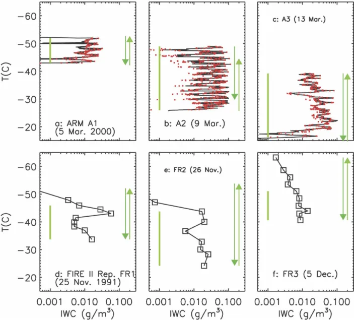
Figures 3–5 provide an overview of the vertical dis-tribution of IWC as a function of temperature for 18 of the 19 cloud profiles. (Spiral A4 is not plotted so as to reduce the number of figures.) Note the fluctuations in the IWC during the aircraft descents (e.g., Fig. 3b): this is due to the aircraft spiraling in and out of generating cells and is an unavoidable issue with aircraft spirals

1_{Lagrangian spiral descent is not ideal for characterizing the}

instantaneous vertical distribution of cloud properties. However, if a source region near cloud top is relatively steady state and vertical wind shear is not appreciable, the microphysical proper-ties sampled downward through the cloud layer can be used to approximate the vertical structure. Unfortunately, a source region is usually small in the horizontal so that fluctuations in the micro-physical properties can be expected during each loop of a spiral.

(5)

through cloud layers. The IWC fall in the range 0.001– 0.3 g m⫺3. The exceptions are cases CF2 and CF4, with IWC⬃ 1 g m⫺3.

The vertical bars on the sides of each panel in Figs. 3–5 provide information on the penetration depth of vertically pointing lidar (right) and radar (left) for the cloud layers (see legend, Fig. 4i). Given that a lidar beam is occulted at an optical depth of approximately 3 (Kinne et al. 1992), the layers in Figs. 3a–c can be fully penetrated by upward (ground based) and downward (e.g., spaceborne) lidar. Similarly, the CloudSat 94-GHz radar, with a detection threshold of ⫺28 dBZe,

would see through the depth of these cloud layers. (The method used to derive Zeis discussed at the end of this

section and in appendix A.) Few points had reflectivi-ties above 0 dBZe, indicated by dark boxes on the left

vertical bars.

The method to calculate the IWC and dBZeis best

shown by first using examples from ARM IOP spiral descents A1–A3. Figures 3a–c plot the IWCs measured directly by a counterflow virtual impactor (CVI) probe (Twohy et al. 1997). Also shown in the panels (red symbols) are points representing the IWCs derived from the PSD (FSSP ⫹ 2D probes), with mass–

FIG. 1. (a) Measured temperatures and (b) derived radar reflectivities for 19 vertical profiles through ice clouds in four field campaigns. Each aircraft “point” represents data from 5 s of aircraft sampling or about 750 m of horizontal path. Each balloonborne point represents 25 m vertically. In (a), initial temperature for each profile is shown with open squares, the flight identification is shown below squares. At the bottom of (a), filled circles show flights from FIRE I (F), filled squares from ARM 2000 IOP (A), except where the star-shaped symbol represents three ascents from balloonborne replicator during FIRE II (FR), and filled tri-angles from CF. In (b), radar reflectivities are for 95 GHz (blue), 35 GHz (green), and 9.6 GHz (yellow).

138 J O U R N A L O F A P P L I E D M E T E O R O L O G Y A N D C L I M A T O L O G Y VOLUME47

Fig 1 live 4/C

(6)

dimensional relationships scaled to agree with the mea-sured IWC when the IWC is above the CVI detection threshold of about 0.01 g m⫺3(see H07a). The mass–di-mensional relationships (m ⫽ aDb) derived from the scaling process are used directly to produce reliable IWCs only when the measured values fall below the CVI’s detection threshold, as evidenced by application of these relationships to more recent datasets where the CVI threshold was⬃0.001 g m⫺3. H07a parameterizes the results of the scaling process. The coefficient a in the m(D) relationship has been represented in terms of temperature a(T) and the exponent b is evaluated using vertically pointing Doppler radar observations for cases A1, A4, and many other ARM observations (Heyms-field et al. 2007b, hereinafter H07b). Temperatures in these three cases spanned the range from⫺50° to ⫺20°C (and for a case not shown, 12 March, to 0°C). The IWCs measured for the three cases are relatively constant with temperature and fall primarily in the range from 0.001 to several tenths of a gram per meter cubed.

Table 1 summarizes the application of the tempera-ture-dependent mass–dimension relationships to the ARM 2000 spirals themselves. The median and mean values of the ratio r⫽ IWC (PSD)/IWC (measured) are case dependent and are generally accurate to within 10%. The greater difference noted for the 9 March case is largely due to CVI measurement error. Sampling during this case was in and out of generating cells and the associated trails. The CVI exhibits hysteresis: water vapor remains inside the instrument’s housing, leading to small underestimates within the IWC region and greater overestimates when the IWC decreases rapidly, as was the case on 9 March. Note also that for a small

minority of the periods during the spirals except for 5 March, the IWC fell below the CVI detection threshold (number of instances, Table 1) and were subsequently derived from the m(D) relationships together with the PSD.

Also note from Table 1 that the IWC in FSSP (small particle) sizes amounted to 12%–17% of the total IWC. The IWC in small particle sizes was considered in the derivation of the m(D) relationships, and although the precise value of the IWC in small particles is not well known, the error resulting from the addition of the FSSP IWC for those cases falling below the CVI detec-tion threshold and for the FIRE I cases is at most 15%. Note that two cases A1 and A4 did not have supporting FSSP data. This would lead to an underestimate of the IWC for those periods when the IWC fell below the CVI’s detection threshold.

Particle habits were predominantly bullet rosettes and rosette aggregates for ARM cases A1–3. For that reason, we can use the same values for a(T ) and b found for the ARM cases to estimate the IWC for the remaining midlatitude, synoptically generated ice cloud layers (cases F1–F8 and FR1–3). From Table 1, given that the particle habits from the FIRE cases are the same as for the ARM cases, we can expect that the application of the m(D) relationships to the FIRE I and II datasets will produce a mean error of⫾10%.

As shown in Figs. 3d–f and 4a–h, the profiles of IWC for the synoptically generated cirrus exhibit consider-able structure. The warmer temperature ice cloud lay-ers were optically thick enough that a lidar beam was unable to penetrate the depth of several of these layers (see Sassen et al. 1994, who reported lidar observations for the FIRE cases). The reflectivities also reach 0 dBZe

and above, highlighted by the dark vertical bars on the left side of the panels, in some instances. For the warmer case A4 (not plotted), where spatial-type ice crystals including bullet rosettes dominated, an a(T ) relationship appropriate for the range of temperatures considered was developed and evaluated on the basis of the four ARM cases.

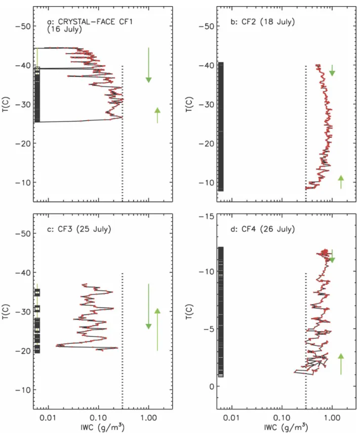
The IWCs from the four CF cloud layers sampled at temperatures from⫺45° to 0°C were measured directly rather than inferred from an m(D) relationship because the CVI detection threshold was usually exceeded (Table 1). We derived a(T ) and b(T ) in the m(D) re-lationship and compared the IWC derived from the PSD with those measured. The ratios are nearly unity except for the 18 July case where there were no FSSP PSD to include in the PSD estimate (Table 1).

The ice clouds sampled during CF had large IWCs and changed little in the vertical, indicating that they were primarily regions of fallout. In general, these

FIG. 2. IWP as a function of optical depth for 19 cloud profiles. For ARM and CF observations, IWP are primarily from direct measurements, and for the other cases, from the particle probes. Extinction is derived from the particle probes.

(7)

clouds were optically thick, inhibiting lidar penetration into the cloud layer. The radar reflectivities above 0 dBZe, as indicated by the bars on the left side of each

panel in Fig. 5, extend throughout the layers.

The participants received estimates of the radar re-flectivities, derived from the PSD and m(D) relation-ships for frequencies of 9.6, 35, and 95 GHz (see Fig. 1b and the discussion in appendix A). (A frequency of 95 rather than 94 GHz is used in the remaining part of this paper to conform to retrievals reported in the litera-ture, although differences for frequencies of 94 and 95 GHz are negligible.)

For midlatitude clouds, we used the Mie scattering estimates for spherical particles from Bohren and Huff-man (1983). This method was chosen because the par-ticles sampled were quasi-spherical: bullet rosettes with some aggregates of rosettes. Using a discrete dipole approximation for different crystal shapes, including quasi-spherical ice particles, Okamoto (2002) found that shape influences on Zeare less than 2 dBZe for

ensemble (PSD) volume-equivalent effective radii of less than 100 ␮m. This criterion was satisfied for all of the midlatitude PSD. The dual-wavelength ratio, dWR ⫽ dBZe (35 GHz)/dBZe (95 GHz), calculated FIG. 3. Vertical distributions of IWC from Lagrangian spiral descents during (a)–(c) ARM 2000 IOP and (d)–(f) balloonborne ice crystal replicator ascents through cirrus during FIRE II. Spirals/ascent codes used in Fig. 1a are shown in each panel. In (a)–(c), the black solid line shows CVI-measured IWC; red dots show those derived from the particle size distributions, scaled according to the measurements, and are used exclusively where IWC fall below the CVI detection threshold. Legend for vertical bars is shown in Fig. 4i and is discussed in the text.

Fig 3 live 4/C

(8)

FIG. 4. As in Fig. 3, but for FIRE I Lagrangian spiral descents. No IWC measurements were made; therefore IWC are estimated from the PSD. Legend is shown in (i).

Fig 4 live 4/C

(9)

FIG. 5. As in Fig. 3, but for CF spirals. Legend for vertical bars is shown in Fig. 4i. Vertical dotted line corresponds to the abscissa of the right edge of plots in Figs. 3 and 4.

Fig 5 live 4/C

(10)

from the midlatitude PSD, is generally less than a few

Zedecibels (Figs. 6a and 1b), indicating that errors

re-sulting from the Mie scattering effects are generally negligible. The largest dWR values are for 12 March 2000 (spiral A4). In Fig. 6b, the measured dWR sampled by a ground-based radar on 12 March 2000, including the period of the spiral (see H07b), follow the same distribution with Ze and has approximately the

same magnitudes as in the calculations.

An estimate of the magnitude of the error of the derived midlatitude radar reflectivities given for the evaluations can be estimated by using the PSD from the four ARM spirals. The masses of all ice particles were increased by 10%, thereby increasing the IWC by an equal amount, expressing a reasonable degree of un-certainty in the CVI measurements and in the FSSP-sized particles. The net increase in radar reflectivity was only 0.65⫾ 0.34 dBZe. On the basis of this sensitivity

study and 1) because the midlatitude particles are quasi-spherical with negligible Mie effects, 2) the mass– dimension relationships produce accurate IWC (Table 1), and 3) there is reasonably good agreement between the calculated and measured reflectivities (H07b), we conclude that the Zederived from the forward model

are probably accurate to 1 dBZe.

Non-Rayleigh effects are significant for the CF clouds (Fig. 1b) that were dominated by aggregates of complex crystal shapes. It is reasonable to assume that the CF particles that dominate the radar reflectivity are horizontally aligned aggregates of aspect ratio (height to diameter) equal to 0.6 based on the observations of Magono and Nakamura (1965) and Hanesch (1999). Matrosov et al. (2005) have developed aT-matrix scat-tering model that adequately describes the radar polar-ization backscattering properties of most nonspherical (oblate) atmospheric hydrometeors, including ice cloud particles, pristine snowflakes, and raindrops. Our for-ward model uses the Matrosov et al. (2005) model with an assumed particle aspect ratio of 0.6.

The few large particles sampled by the particle probes dominate the reflectivity. In H07a, we report on an evaluation of the influence of the statistics of the PSD on Ze. Statistical variation of the ice particle

con-centrations in the largest sizes is used to evaluate the effects on Ze. There is essentially no net bias in the

calculated Zeresulting from the statistics of the small

sample, although in the retrievals this could lead to increases in the statistical uncertainty in IWC derived from spaceborne platforms.

The ensemble, reflectivity-weighted fall speeds VZat

the three radar wavelengths and for Rayleigh scatterers were calculated from the masses and terminal velocities of the ice particles integrated across the PSD. H07b describe the methodology and compare the estimated distribution of VZwith reflectivity with that measured

by vertically pointing Doppler radar on two of the days used in this algorithm evaluation (A2 and A4). In ap-pendix A, we discuss the impact of errors in our esti-mates of VZon the retrieved IWC.

The volume extinction coefficient in visible wave-lengths␴ was supplied for those participants employing a lidar–radar approach. The ␴ were estimated from twice the total particle area per unit volume in sizes from FSSP (assuming the particles were spherical) through to the largest particles measured by the imag-ing probes (based on the particle cross-sectional areas). Heymsfield et al. (2006) compare estimates of␴ from the particle probes with those measured by the cloud integrating nephelometer (CIN) probe (Gerber et al. 2000) from CF. The ␴ from the CIN are, on average, about 2 times those derived from the particle probes. Heymsfield et al. (2006) provide reasons why the par-ticle probe estimates are likely to be more reliable than those from the CIN, although we are not confident about the contribution from the FSSP. The potential impact of errors in␴ on the retrieved IWC can be es-timated by assuming, for example, that␴ are over- or underestimated by 20% but that the radar reflectivity

TABLE1. Application of mass–dimension relationships to ARM 2000 IOP and CF 2002 spirals. [For the FIRE-I (cases F1–8) and FIRE-II Replicator cases (FR1–3), there were no direct measurements of the IWC.] The asterisk indicates IWC(Meas)⬍0.005 g m⫺3.

Date

IWC(PSD)/IWC(Meas)

Total No. of points

Points below

CVI threshold* Ratio IWCFSSP/IWCmeas

Median Mean Std dev

5 Mar 2000 (A1) 1.07 1.08 0.16 231 121 No data

9 Mar 2000 (A2) 0.88 0.89 0.26 601 38 0.17

13 Mar 2000 (A3) 0.93 1.0 0.30 311 29 0.13

12 Mar 2000 (A4) 0.93 1.0 0.30 216 44 No data

16 Jul 2002 (CF1) 0.95 1.04 0.64 281 3 0.12

18 Jul 2002 (CF2) 0.85 0.84 0.11 301 1 No data

25 Jul 2002 (CF3) 1.02 1.09 0.29 151 1 0.11

26 Jul 2002 (CF4) 0.99 1.04 0.26 311 1 0.12

(11)

supplied to the investigators is exactly correct. Taking the FIRE cases (F1–F8) as an example, the Donovan and van Lammeren (2001) radar–lidar method predicts an increase in the IWC of 1.178 ⫾ 0.014 g m⫺3 (for ␴ ⫽ ⫹20%) and a decrease of 0.85 ⫾ ⫺0.01 g m⫺3

(␴ ⫽ ⫺20%). [Potential systematic overestimates in the ␴ provided to the investigators resulting from shatter-ing on the inlet of the FSSP probe (Field et al. 2003) are evaluated in appendix B and quantified in Table B1.] Note that FSSP data were unavailable for cases A1, A4, and CF2.

3. Results

Eight teams, some with more than one IWC retrieval method, participated in this study. They were provided

with vertical profiles of temperature (T ), Zeat

frequen-cies of 9.6, 35, and 95 GHz, reflectivity-weighted fall speeds (VZ) at these wavelengths ␴ and an optical

depth␶ as derived from ␴ integrated downward from cloud top and upward from cloud base. The vertical resolution of the profiles was⬃5 m.

Table 2 summarizes the IWC retrieval methods and the publications that describe their methodology, grouped between dark horizontal lines according to the methods used. Most of the algorithms use gamma-type particle size distributions but several use normalized PSD represented in terms of the melted equivalent di-ameter. The algorithms include the use of Ze alone

[1(Z95)], Zeand␶ [2(⌮95_⌷D)], Zeand T [3(ZT)], Ze

and ␴ [4(LiRad)], lidar–radar approach), and Zeand FIG. 6. Comparison of dual-wavelength ratio [dBZe(35)/dBZe(95) GHz] as a function of Ze

at 35 GHz derived from (a) midlatitude PSD and (b) ARM SGP 2000 IOP, from University of Massachusetts radars on 12 Mar 2000.

(12)

T ABLE 2. Summary of participant evaluation methods. Rules between rows delinea te each family of methods (radar only, radar – optical depth, radar – temperature, radar – lidar, and Doppler radar). Here ␮ is dispersion of gamma PSD; NT ⫽ total number concentration of gamma PSD. Participant Reference number and type Required data-radar (wavelength) PSD Mass (D ) relationship Habit Non-Rayleigh effects Range of applicability Austin a 1a – radar – only (Z95) Reflectivity (95 GHz) Gamma, retrieving constant ␮ , and NT in column Ice spheres Spherical Mie correction ⫺ 40 to 10 dB Z (95 GHz) Austin a 2a – radar visible optical depth (Z95_OD) Reflectivity (95 GHz), visible optical depth See above Ice spheres Spherical Mie correction ⫺ 40 to 10 dB Z (95 GHz) Protat/ Delano ë b 3a – radar, temperature (Z95T) Reflectivity (95 GHz), temperature Normalized N0 c BF95 Spherical Mie correction Temperature: ⫺ 60 ° to ⫺ 5 °C, ⫺ 50 to 10 dB Z Hogan d 3b – radar, temperature (ZRayT) Reflectivity (Rayleigh, temperature) Gamma, ␮ ⫽ 2, adjusted to account for ice crystals ⬍ 100 ␮ m BF95 Spherical No Temperature: ⫺ 5 ° to ⫺ 55 °C, ⫺ 30 to 20 dB Z Hogan 3c – radar, temperature (Z95T) Reflectivity (95 GHz), temperature See above BF95 Spherical Mie correction ⫺ 30 to 5 dB Ze Wang e 4a – radar – lidar (LiRad95) Extinction, reflectivity (95 GHz) Gamma ( ␮ ⫽ 2) BF95 Various habits No Ze ⬍ 20 dB (35 GHz), ⬍ 10 dB Z (95 GHz), ␶ ⬍ 3 Van Zadelhoff/ Donovan f 4b – radar – lidar (LiRad35) Lidar backscatter (extinction), reflectivity (35 GHz) Modified gamma ( ␮ ⫽ 2) BF95 Various habits No ⫺ 50 to 20 dB Z (Rayleigh), ␶ ⬍ 3 Okamoto g 4c – radar – lidar (LiRad95) Lidar backscatter (extinction), reflectivity (95 GHz) Modified gamma ( ␮ ⫽ 2) Solid ice sphere Mie ␶ ⬍ 3 Bouniol h 4d – radar – lidar (LiRad95) Extinction, reflectivity (95 GHz) Normalized N0 b BF95 N/A No ␶ ⬍ 3 Delano ë / Protat i 5a – Doppler radar (Z95V Z ) Reflectivity (95 GHz) Doppler fall speed Normalized N0 b Retrieved Retrieved from five typical habits Homogeneous spheres, but ice density adapted in Mie calculation to fit retrieved particle habit Temperature: ⫺ 60 ° to ⫺ 5 °C; ⫺ 50 to 10 dB Z Sato j 5b – Doppler radar (Z95 VZ ) Reflectivity (95 GHz), Doppler fall speed Modified gamma ( ␮ ⫽ 2) HM03 k (hexagonal columns and rosettes) Nonspherical ice DDA Ze ⬍ 0 dB (95 GHz) aNew form based on Austin and Stephens (2001) and Benedetti et al. (2003). bProtat et al. (2007). cDelano ë et al. (2005). dHogan et al. (2006a). eWang and Sassen (2002a,b). fDonovan and van Lammeren (2001). gOkamoto et al. (2003). hTinel et al. (2005). iDelano ë et al. (2007). jSato and Okamoto (2006). kHeymsfield and Miloshevich (2003).

(13)

VZ[5(Z95VZ)]; the “Doppler radar” approach). Note

that some of the lidar–radar retrieval algorithms re-quire direct estimates of extinction (e.g., Wang and Sas-sen 2002a,b) whereas others have the desirable feature that they use lidar backscatter directly (e.g., Donovan and van Lammeren 2001; Okamoto et al. 2003). The latter methods have been modified to use our extinc-tion estimates.

The accuracy and applicability of the various ap-proaches to the range of conditions sampled in this

study can be evaluated by comparing the “retrieved” IWC (IWCretr) with those “measured” (IWCmeas,

shown in Figs. 3–5). The latter were either measured by the CVI, or, when below its detection threshold or oth-erwise unavailable (FIRE I, FIRE II replicator), esti-mated from the PSD and m(D) relationships.

Figures 7 and 8 show the ratio r⫽ IWCretr/IWCmeas

for the five approaches encompassing all teams, plotted as a series of 5-s data points along the abscissa, as in Fig. 1. The results differ widely amongst approaches.

Com-FIG. 7. Ratio of retrieved-to-measured IWC, with abscissa as in Fig. 1, for algorithms groups 1, 2, and 3 (see Table 2). The method employed and the median and the variance about the mean values for each approach are shown and plotted. The legend and position of each flight appears in (d). Symbols correspond to field program from Fig. 1.

(14)

parable mean values of r averaged for all data points (listed in each panel) are obtained for approaches 1a(Z95) and 2a(Z95-OD) used by team 1 (Figs. 7a,b), producing good estimates of the IWC in a mean sense but with a large standard deviation. Their radar-only approach 1a(Z95) produces IWCs that are significantly underestimated for the low temperature midlatitude cases A1 and FR1–FR3, and are much improved with the addition of optical depth 2a(Z95_OD). It is also noteworthy that approach 2a produces IWC that are nearly equal to the measured values (r⬃ 1) for the CF cases, unlike the results for the other methods. The

results for method 3(ZT) are either biased high (Figs. 7c,f) or have a large standard deviation (Fig. 7e). The lidar–radar methods 4(LiRad) show mean values of r of nearly unity and with relatively low standard devia-tions. The results for 4a(LiRad95) are close to unity throughout (Fig. 8a) with the exception of the CF cases with appreciable Mie effects (not considered in this algorithm), where the IWCs are significantly over-estimated. Underestimates are noted for the low tem-perature, FIRE II replicator cases. The results for 4b(LiRad35) are nearly unity throughout (Fig. 8b), ex-cept for significant underestimates for the low

tempera-FIG. 8. As in Fig. 7, except that one set of results is shown for groups 4–8.

(15)

ture spiral CF2, with significant numbers of large par-ticles. The results for 4c(LiRad95) agree well with the measured values (Fig. 8c), with a mean value near unity and with a low standard deviation. The results for 4d(LiRad95) are biased low throughout (Fig. 8d) ex-cept for the ARM cases. Note that the extinction values provided to investigators 2a and 4a–d may be overesti-mated because of shattering of large particles on the inlet of the FSSP probe (an issue addressed in appendix B and Table B1).

Use of Zeand VZ by 5a and 5b (Z95VZ) produces

values of r of nearly unity throughout (Figs. 8e,f); how-ever, the IWC is significantly underestimated (espe-cially for 5b) for the CF cases exhibiting appreciable Mie effects, which are treated differently by 5a and 5b. The ratio r for each method and team has been ex-amined in different ways to identify weaknesses and limitations in the retrieval algorithms. Some variables add insight (e.g., temperature); other variables, which may not be independent (e.g., Zeand IWC), place

geo-physical limits on accuracy. The evaluations are pre-sented in Figs. 9–15 and the results are summarized in Fig. 16, according to method. We arbitrarily choose the range 0.75⬍ r ⬍ 1.25 to represent “good” agreement between the retrievals and measurements, given the un-certainties in the parameters, especially␴, supplied to the investigators. Outside of this range, there are biases suggesting weaknesses in a given approach. Note that a lidar beam is occulted at an optical depth of about 3 and CloudSat, for example, cannot detect cloud below⫺28 dBZe. (Figure 16 considers these detection thresholds.)

To reduce the number of figures, the more sophisti-cated method for each team is chosen for these evalu-ations.

No strong biases of r with Ze are noted for

2a(Z95_OD) (except for reflectivities below the Cloud-Sat threshold, Fig. 9a), 4c(LiRad95) (Fig. 9c), 5a and 5b (Z95VZ) (Figs. 9g,h), except for 5b at large Ze(Fig. 9h).

The greater bias for large Zefor method 5b with respect

to method 5a is consistent with the findings shown in Fig. 8 and may be related to a different treatment of the Mie effect (discrete dipole approximation in method 5b versus homogeneous spheres with corrected ice density in method 5a). Results from methods 4b(LiRad35) and 4d(LiRad95) (Figs. 9d–f) show an increasing low bias of IWCretrwith increasing Ze, for reasons related to using

Rayleigh scattering and/or the mass–dimension rela-tionship chosen for their algorithm (from Brown and Francis 1995, hereinafter BF95). At higher reflectivi-ties, 10 dBZe and above, the results from methods

3c(Z95T) and 4a(LiRad95) are overestimated (Figs. 9b,c). The treatment of nonspherical particles and Mie

effects or the assumed breadth of the PSD may be the possible cause of these positive biases.

Biases in r as a function of the IWC are less pro-nounced than with Ze(Fig. 10). At low IWC, the results

for 2a(Z95_OD) are appreciably overestimated and those of 3c(Z95T) are biased high, especially for the higher IWC; these trends are consistent with the trends noted for Ze. The results for 4d(LiRad95) are generally

underestimated. Particularly low standard deviations are noted in the results for 4a, 4c, 5a, and 5b. Because a given IWC can be found over a wide range of tem-peratures, these low standard deviations suggest that these methods account properly for temperature.

There are few biases noted when the data are parti-tioned according to temperature (Fig. 11). The results for approach 2a(Z95_OD) for temperatures of⫺45°C and below are biased low, whereas those of 3c(Z95T), where temperature is a primary input variable, show a tendency to underestimate the IWC at low tempera-tures and overestimate it at warm temperatempera-tures. The above results are clearly consistent with those found in Figs. 9 and 10. The same result for this method was found at temperatures below ⫺35°C by Hogan et al. (2006a). Method 4a(LiRad95) overestimates the IWC at temperatures above⫺10°C, not because of incorrect treatment of temperature but primarily because the Rayleigh approximation and the BF95 mass–dimension relationship were used. Methods 4c and 5a produce val-ues of r of nearly unity for all temperatures, whereas those for 4d are biased low, mirroring earlier findings. Relatively low standard deviations are shown for groups 4c, 5a, and 5b, likely indicating that for a given temperature the PSD parameterizations and the treat-ment of the scattering signature in the Mie region are good.

As a lidar beam is occulted at an optical depth of about 3, an examination of how the lidar–radar ap-proach performs at optical depths integrated from cloud top downward into cloud until␶ ⫽ 3 is useful for assessing the accuracy of the lidar–radar approach un-der real conditions. All of the lidar–radar methods show little bias in the optical depth range 0.1–3 (Fig. 12), with the exception of those for 4d. It is noteworthy that if more penetrating lidars could be developed, li-dar–radar methods presently available would still have the same level of accuracy at higher optical depths.

Figures 13–15 examine factors that might point to errors in the way the various methods treat the particle size distributions. Most of the retrieval algorithms are based on gamma-type PSD,

N共D兲⫽ N0D␮e⫺␭

D

, 共1兲

(16)

where N0is the intercept parameter, D is the ice

par-ticle maximum diameter, ␮ is the dispersion, and ␭ is the slope. The lidar–radar approach implicitly elimi-nates the need for N0because Zeand␴ are each

pro-portional to it, indicating why this method should be inherently more accurate than the other methods.

Distance into the cloud layer alters the PSD through aggregation, broadening it and reducing␭ and N0. In

FIG. 9. Ratio of derived-to-measured IWC as a function of equivalent radar reflectivity Ze.

(17)

Fig. 13, the ratio r is examined as a function of distance below cloud top. (For case CF4, cloud top was not reached; the data, almost all above⫺10°C, are used in Fig. 13 for completeness.) The greatest biases are found

for method 3c(Z95T) and to a lesser extent for 4d(LiRad95). The results for 2a, 4a, 4b, 4c, 5a, and 5b show little bias with depth below cloud top, implying that representations of the PSD are accurate. The low

FIG. 10. As in Fig. 9, but for IWC.

(18)

standard deviations for the lidar–radar approach dem-onstrate the merits of this approach, which removes errors by eliminating assumptions of N0. The same is

not true for method 2a(Z95_OD), which exhibits large

standard deviations. In layers deeper than about 4 km, mostly from the CF cases, the results for methods 3c(Z95T) and 4a(LiRad95) are overestimated and those of 4b and 4c are slightly underestimated, largely

FIG. 11. As in Fig. 9, but for temperature.

(19)

as a result of how Mie effects in the radar part of the retrieval algorithm were considered. The results for 4d are negatively biased throughout.

We now evaluate whether the assumed values of the

PSD parameters [Eq. (1)] used by the various retrieval algorithms lead to biases. Most of the retrieval algo-rithms use␮ ⫽ 2.0. The dispersion of the PSD fitted to our data using the first, second, and sixth moments

ex-FIG. 12. As in Fig. 9, but plotted according to the optical depth integrated from cloud top downward to the measurement level.

(20)

hibit␮ ranging from about ⫺2 to ⫹4, with a mean of 0.16⫾ ⫺1.6 and a median of ⫺0.08 (essentially an ex-ponential PSD). In Fig. 14, the ratio r is examined as a function of the␮ derived from the measured PSD. In

this comparison, we are not separating out other ef-fects, such as the slope of the PSD; we do that below. Although there is sensitivity noted for the results for 3c9 (Z95T) and 4d, it is modest. Because the lowest

val-FIG. 13. As in Fig. 9, but for distance below cloud top.

(21)

ues of␮ are associated with the warmest temperatures in which Mie effects are significant (case CF4), and because method 4a did not consider Mie effects, the increase in error for method 4a where ␮ ⬍ 1 is not

related to␮ directly. We conclude from this compari-son that the choice of␮ is not negatively affecting the retrievals, although refinements could reduce the stan-dard deviation of the estimates.

FIG. 14. As in Fig. 9, but for dispersion␮of the gamma distributions fit to the data. Binning intervals are in equal intervals of number of points.

(22)

FIG. 15. As in Fig. 9, except shown as a function of IWC/Ze. Horizontal bars along the right side of each plot show the mean dWR

[Ze(Rayleigh)/Ze(95 GHz)], with methods used to calculate each discussed in section 2. The right side of each panel shows the

dual-wavelength ratio, with the scale for horizontal bars given in (h).

(23)

We can also infer whether the ␭ values used by the various groups have produced some of the errors

noted in the retrieved IWC. From Heymsfield et al. (2005), IWCⲐZe共g mm⫺6兲⫽ ␲2_␭b 共␳0兲 2 兵36⫻ 106_ar mie关1.09共KiⲐKw兲 2_兴_其_关_⌫_共_b_{⫹ 1 ⫹}_␮_兲_Ⲑ⌫_共_2b_{⫹ 1 ⫹}_␮_兲兴共2兲

where ␳0 is the density of liquid water, the term in

parentheses with Kiand Kwconverts the radar

reflec-tivity with respect to solid ice to the equivalent radar reflectivity, a and b are the coefficient and exponent in the mass–dimension relationship, and rmieis the ratio of

the radar reflectivity for a given wavelength to the ra-dar reflectivity for Rayleigh scatterers. In Eq. (2), we use the BF95 m(D) relationship,␮ ⫽ 2, and a radar wavelength of 95 GHz to correspond to the input pa-rameters used in 3c(Z95T), 4a, and 4b. For rmie, we use

our results for 95 GHz.

A systematically increasing positive bias in r with de-creasing IWC/Zeis noted for approach 3c(Z95T), and

to a lesser extent 4a(LiRad95) (Fig. 15). The biases are a function of the Mie effect (where IWC/Ze⬍ 0.07; see

horizontal bars on the right side of each panel in Fig. 15). If we use rmie⫽ 1 (Rayleigh scatterers), in Eq. (2)

the biases largely disappear. Because the trend noted is not due directly to errors in the treatment of ␭, the primary discrepancies noted in Fig. 15 are therefore due to the treatment of Mie effects and not␭.

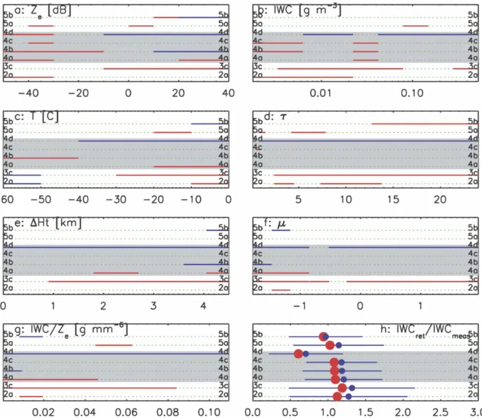
The biases found in Figs. 9–15 are shown graphically in Fig. 16. The biases are most prominent in the evalu-ations partitioned according to the radar reflectivity and IWC (Figs. 16a,b). At high reflectivities, we at-tribute differences in the retrieved and measured IWC to be primarily due to whether or how Mie and non-spherical particle scattering is treated. At low reflectivi-ties, almost all approaches overestimate the IWC. This almost certainly has its roots in overestimated masses ascribed to small particles. Method 4d(LiRad95) is bi-ased low for all metrics. The intercept parameter N0of

the PSD is not at fault because r does not trend with IWC/Ze. The mass–dimension relationship is not at

fault because the BF95 relationship used is the same as the other LiRad approaches. We therefore conclude that the slopes of the PSD are biased high. High biases in r are noted for approach 3c(Z95T).

Figure 16h summarizes the results of the evaluation for all retrieved IWC, not partitioned by any variables but with radar and lidar thresholds considered. The ap-proaches that use the lidar–radar combination, con-tained within the shaded regions, and the Doppler ra-dar approaches (upper part of the figure) have a ratio of retrieved-to-measured IWC of nearly unity, with low

standard deviations. These results demonstrate the util-ity of the LiRad approach. Methods 2a(Z95_OD) and 3(ZT) [directly applicable to the Aqua satellite constel-lation (A Train) datasets] produce good results overall, but the standard deviations are much larger (about a factor of 2 for IWC) than for the LiRad approach.

Values of the visible extinction coefficient provided to the investigators included contributions from par-ticles sampled by the FSSP probe, although there were exceptions noted earlier. There may have been signifi-cant contributions to ␴ from large ice particles that shattered on the inlet of the FSSP—that is, artifacts. As shown in appendix B (and quantified in the second and fourth columns of Table B1), this might have resulted in up to a 25% uncertainty in the ratio of the retrieved-to-measured IWC. Overall, the results are still excel-lent.

Accurate retrievals of the IWC and IWP are central to improving the representation of ice clouds in climate models (Stephens et al. 2002). In Fig. 17, the IWP ob-tained using the results from the various groups are compared with the measured values for the 19 cases. Two sets of results are shown in the figure that pertain specifically to CloudSat–CALIPSO: 1) those for those portions of the cloud layer where the “measured” re-flectivity exceeds⫺28 dBZe, to simulate what CloudSat

would measure (CloudSat only), and 2) those for por-tions of the cloud layer where 1) is satisfied and where the cloud optical depth is 3 or less. The dropoff of IWPretr/IWPmeas with increasing IWPmeas occurs

be-cause the IWPretr remains constant when an optical

depth of 3 is reached and the IWPmeascan continue to

increase beyond that point. Also listed and plotted in each panel are the mean ratio IWPretr/IWPmeasand its

standard deviation, reflecting how accurately each re-trieval algorithm estimated the IWP through cloud depth. In considering IWPretr/IWPmeas, the results for

2a(Z95_OD) (the standard CloudSat algorithm) are good overall. The mean ratio of predicted-to-measured IWP is nearly unity and the standard deviation is rela-tively small. The results for 3c(Z95T) follow the earlier patterns: underestimates at the low IWPs and overesti-mates at the high ones, which translate into an overes-timation by 20% of IWP. LiRad retrievals yield good results overall, except for errors induced where tem-156 J O U R N A L O F A P P L I E D M E T E O R O L O G Y A N D C L I M A T O L O G Y VOLUME47

(24)

peratures are warm and Mie effects are large. For ex-ample, method 4d produces underestimates at low IWP. Results for 5a([Z95VZ) are good overall, with a

slight positive bias of IWP but a relatively small stan-dard deviation. The results from 5b(Z95VZ) produce

the best estimates of IWP among all methods.

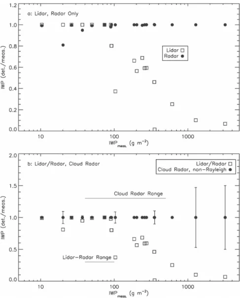
Figure 17 also shows that a lidar–radar approach, if used alone, would drastically underestimate the IWP for the clouds with large IWP. The figure also suggests that accurate approaches are needed to derive the IWC from lidar at low IWP (when radar begins to fail to detect cloud) and from radar at high IWP (when the lidar beam is occulted). These points are illustrated

graphically in Fig. 18a, which considers fictitious “per-fect” retrievals, making the results independent of the approaches used by the study participants. The meth-ods used in this figure include lidar alone (measuring from above cloud with the beam occulted at an optical depth of 3), 95-GHz cloud radar alone (with a minimum detectable reflectivity of⫺28 dBZe), and a combination

of the two. We assume that the IWC is retrieved per-fectly from the measurements meeting the detectability limitations and refer to this as IWCdet(detected). An

additional scenario assumes that the cloud radar has the same minimum detectable reflectivity, but at Zeof 6

dBZeand above there is a⫾50% error in the retrieved FIG. 16. Summary of results from Figs. 9–15. The abscissa is the variable in the top left corner of each panel, with units given in brackets rather than below the axis to conserve space. The algorithm identifier is shown along the ordinate, extending across the plot with dotted lines. The shaded region is for algorithms using a lidar–radar approach. In (a)–(g), red and blue bars show positive and negative biases⬎25%. In (h), red dots show median values of ratio of retrieved-to-measured IWC; blue dots and horizontal bars show mean and std dev. The dots are subsets in the following way: lidar–radar,␶⬍ 3, Ze⬎ ⫺28 dBZ; all others, except Doppler approaches

5a and 5b, 8: Ze⬎ ⫺28 dBZ.

Fig 16 live 4/C

(25)

FIG. 17. Ratio of retrieved-to-measured IWP as a function of the IWP for the 19 cloud layers used in this study, organized as in Figs. 9–15. Solid black circles show ratio of retrieved-to-measured for the portion of the cloud column with reflectivities above⫺28 dBZ (which is virtually the same as for the total cloud column, which is not plotted for clarity), and times signs show the ratio for the portion of the cloud where the reflectivity is above⫺28 dBZ and the optical depth is 3.0 or below. The listed and plotted mean and std dev (solid line, mean; dotted line, std dev) are derived from the ratio for the entire cloud column.

(26)

IWC, resulting from uncertainties in how to treat non-spherical ice particles and non-Rayleigh scattering based on the dWR estimations in Fig. 6 and the findings shown in Fig. 9. When the IWP reaches about 100 g m⫺2, the lidar beam begins to occult, a diminishing por-tion of the IWP would be measured, and cloud radar would underestimate the IWP below about 40 g m⫺2.

Figure 18b shows that, when considered together, the LiRad approach yields accurate IWP (to within 20%) from the CALIPSO–CloudSat spaceborne remote sen-sors only in the relatively narrow range of 40–100 g m⫺2 (Fig. 18b). The uncertainty in the treatment of the ef-fects of nonspherical ice particles and Mie scattering

for the higher reflectivities measured by cloud radar leads to the result that cloud radar is unable to retrieve IWP ⬎ 500 g m⫺2. Note that there are obvious errors from nonspherical particle effects for the higher IWPs and attenuation (not considered), which is also signifi-cant in the high IWC/IWP layers.

4. Summary and conclusions

This study presents a comprehensive examination of the accuracy and limitations of algorithms used to re-trieve the IWC from radar reflectivity alone and to-gether with estimates of optical depth in visible

wave-FIG. 18. Ratio of detected-to-“measured” IWP for the 19 cloud profiles from this study (a) as sensed by a lidar, which can fully penetrate cloud up to an optical depth of 3, and by cloud radar, which detects above ⫺28 dBZe; (b) jointly for thresholds for lidar and radar (the

lidar–radar approach), and for a cloud radar that accurately senses between⫺28 and 6 dBZe,

and above 6 dBZewith an error of⫾50%.

(27)

lengths, lidar extinction, temperature, and mean reflec-tivity-weighted ice particle fall speed. It includes almost every category of methodology used to retrieve the IWC from radar-based algorithms and includes most but not every investigator working on this problem. The 19 cloud profiles used in the study derive from mid-and low-latitude ice clouds. The 3389 data points in the vertical, separated by⬃5 m, cover a wide range of con-ditions, spanning a temperature range from⫺65°C to 0°C, cloud depths ranging from 1.2 to 4.6 km, optical depths from thin to deep cirrus according to the ISCCP definition (␶ ⬃ 0.5–50), IWC from less than 0.001 to above 1 g m⫺3, IWP from 10 to 3000 g m⫺2, and esti-mated radar reflectivities in the range from⫺50 to 30 dBZeat 9.6 GHz and from⫺50 to 15 dBZeat 95 GHz.

The various methods collectively and individually produced accurate IWC. The mean (median) ratio of all of the user-provided IWCs to the measured values was 1.15 (1.03) ⫾ 0.66. The radar-only and radar– temperature retrievals (methods 1a and 3c) were less accurate, with a mean (median) ratio of 1.29 (1.20)⫾ 0.75. Lidar–radar approaches (methods 4) produced the best results overall, with a mean (median) ratio of 1.08 (1.00)⫾ 0.61 if there was no restriction on the optical depth. If only those periods are considered when the optical depth is less than 3 and the radar reflectivity is ⫺28 dBZe or above to consider CloudSat–CALIPSO

thresholds, this ratio is 1.08 (1.00)⫾ 0.53, demonstrat-ing the utility of the lidar–radar approach. The results were almost as good for the standard CloudSat radar– visible optical depth approach although with a larger standard deviation. To evaluate the impact of potential errors in the measurement of small (⬍50␮m) ice crys-tals on the retrievals from the radar–optical depth and lidar–radar approaches, the contributions of the small ice crystals to the total extinction were removed com-pletely except when they were obviously real. In this obviously extreme sensitivity study, the results for these approaches were still excellent: the mean (median) ra-tios of the retrieved-to-measured IWCs were 0.81 (0.75) ⫾ 0.44 for the lidar–radar approach and 0.99 (0.84)⫾ 0.75 for the radar–visible optical depth algo-rithm. The Doppler radar retrievals (method 5) as a group also produced almost the same level of accuracy as the radar–lidar method, although these methods are not yet applicable to spaceborne instruments, with a mean (median) ratio of 1.06 (0.98) ⫾ 0.56, and 1.14 (1.03)⫾ 0.60, with the above restriction on radar de-tectability. For actual clouds, the accuracy of the results reported above would be degraded because of attenu-ation of the 95-GHz radar beam, attenuattenu-ation and mul-tiple scattering of the lidar beam, errors involved in the conversion of lidar backscatter to extinction, spatial

av-eraging scales of the radar and lidar beams, and the contribution of vertical air motions to the Doppler ve-locities (for the radar–Doppler fall speed approach).

Researchers participating in this investigation were provided with vertical profiles of radar reflectivity de-rived based on mass–dimension relationships that were constrained by direct measurements of the IWC and evaluated based on coincident radar–Doppler fall speed measurements (H07b). The associated vertical profiles of the extinction coefficient in visible wave-lengths and Doppler fall speeds were derived from par-ticle size distributions. Because Ze, VZ, and␴ were not

measured directly, there are potential errors or uncer-tainties in the values provided to the investigators. In sensitivity studies that evaluated approximate uncer-tainties, varying the IWC by 10% resulted in changes in the Zeby⬍1dBZe, changing the VZby⫾10% yielded

IWC that were uncertain by ⫾25%, and varying the extinction by⫾20% but assuming that the Zewere

cor-rect resulted in an uncertainty of ⫾15%. Removing these uncertainties would reduce the standard devia-tion of the evaluadevia-tions by ⬃15%–20% but would not change the mean values unless there are biases uncov-ered in the instrumentation used to derive Zeand VZ.

New methods are needed to improve the range of utility of the lidar–radar approach and to derive the IWC from cloud radar and lidar alone. Although the lidar–radar approach was found to be more accurate than the other approaches, the range of usefulness of the approach is limited. It is shown from our empirically derived results that this approach can be accurate only within the IWP range from about 40 to 100 g m⫺2, assuming the CALIPSO–CloudSat detection thresh-olds; below that, cloud radar detection threshold be-comes important and above it, a lidar beam is occulted. For IWP above 500 g m⫺2, non-Rayleigh effects be-come so important and are so uncertain that cloud ra-dar alone cannot now be used to reliably retrieve the IWP.

Based on a number of tests designed to uncover weaknesses in the retrieval algorithms (Fig. 16), there are several areas where improvements can be made. A reflectivity–temperature method is potentially useful because it might only require a variable that could, but need not be, measured from a satellite-borne platform; for example, temperature could be derived from Euro-pean Centre for Medium-Range Weather Forecasts (ECMWF) model forecasts. Improvements can be made to the representation of the mass–dimension re-lationship (H07b) by incorporating temperature depen-dence for the a and b coefficients in the m(D) relation-ship. The parameterization for the slope and dispersion of the PSD can be refined using currently available 160 J O U R N A L O F A P P L I E D M E T E O R O L O G Y A N D C L I M A T O L O G Y VOLUME47

(28)

observations that cover a wide range of temperatures. Improvements might also be made through consider-ation of alternate approaches to account for nonspheri-cal particle scattering and Mie effects (e.g., Okamoto 2002; Matrosov et al. 2005). The lidar–radar retrieval methods are accurate to within 10% in a mean sense and with a lower standard deviation and are not in need of major improvement, although the approach is lim-ited. The results for the reflectivity–Doppler fall speed method are accurate and have low standard deviations. This method obviously holds much promise, although it cannot currently be used from satellite-based measure-ments [but there are plans for a European Space Agency Earth Clouds, Aerosols and Radiation Ex-plorer (EarthCARE) mission, provided that Doppler velocity is accurately measured]. The radar–optical depth method, now currently in use for CloudSat re-trievals, produce adequate results, but improvements are needed at the temperatures below ⫺40°C and to refine the assumptions to reduce the standard devia-tion.

A major potential source of error identified here and in earlier studies is the treatment of nonspherical (Mie) effects, most significantly for 94 GHz (which is the fre-quency used for CloudSat and upcoming EarthCARE cloud radars). The differences between the retrieved and “measured” IWC for Ze⬎ 5 dBZewere large, for

some methods overestimating and others underestimat-ing the IWC. This situation occurs primarily at the warmer temperatures. It is not clear whether the method used to estimate nonspherical effects was con-sidered properly here, although indications are that the results are reasonable agreement with observations. An effort needs to be made to establish proper treatment of nonspherical effects for Ze⬎ 5 dBZeand algorithms

to correctly account for attenuation at 94 GHz are also required.

Acknowledgments. The authors thank the CloudSat

Project Office (JPL), especially Deborah Vane, Cloud-Sat Deputy Mission Project Manager, who helped to coordinate and support this research. Support from the MMM Division at NCAR is greatly appreciated. Part of this research was funded through the SRON Program Bureau External Research (EO-052 & EO-083). Thanks are given to Matthew Shupe, Sergey Matrosov, and an anonymous reviewer for their comments.

APPENDIX A

Accuracy of IWC, Ze, and VZProfiles

For cirrus formed in situ in which bullet-rosette-type crystals predominate, the procedure we describe in

sec-tion 2 involving direct measurements of IWC and ver-tically pointing Doppler radar observations leads to an estimated IWC accuracy of ⫾20% for those profiles where the IWC were estimated from the PSD. For the convective cloud cases, the IWC were measured di-rectly; the m(D) relationships are therefore accurate. We therefore have a good handle on the PSD and m(D) relationships for all of the profiles. The primary uncer-tainty concerns the treatment of Mie effects for non-spherical ice particles. Adopting the T-matrix approach of Matrosov et al. (2005) for the convective cloud cases where Mie effects are most significant, we estimate an uncertainty of⫾2dB in radar reflectivity. Conversely, a 2-dB uncertainty in the radar reflectivities given to the groups will lead to only a 4% uncertainty in the IWC based on our direct measurements.

Reflectivity-weighted ice particle fall speeds were de-rived from ice particle mass and fall velocities inte-grated across the PSD, as in H07b. The greatest per-centage differences were noted for measured VZ

be-tween 40 and 60 cm s⫺1, where the calculations were ⬃10–15 cm s⫺1_{lower. To evaluate the potential error in}

IWC derived from VZalone, we fitted the relationship

IWC (g m⫺3)⫽ 0.0036 exp[(VZ(0.0203)] to our

calcu-lations for a radar wavelength of 95 GHz. Taking VZto

be 50 cm s⫺1yields an IWC of 0.011 g m⫺3. Taking this relationship as truth, had we underestimated VZby 10

cm s⫺1, the IWC would have been 25% lower. If the IWC were derived from VZonly, without other

ancil-lary data (such as the radar reflectivity), a perfect re-trieval algorithm would provide IWC that were biased low by⬃25% or less. This calculation also assumes that there is no vertical wind, which obviously must be in-cluded if IWC were derived from VZonly.

APPENDIX B

Influence of Small (FSSP Size) Particles on Lidar–Radar and Radar–Optical Depth Retrievals

The lidar–radar methods 4a–d and the radar–visible optical depth method 2a rely on estimates of the visible extinction coefficient or its integration through cloud depth. Values of␴ were provided to the investigators from the sum of␴ in small (FSSP size) and large (2D size) particles. Exceptions were for cases where no FSSP data were available (A1, A4, CF2), and for the replicator observations (FR1–3), which provided a con-tinuous set of data from small to large ice particles. The true contributions of small particles to␴ from the FSSP is uncertain because of contributions of large ice par-ticles that shatter on the probe’s inlet (Field et al. 2003). The FSSP probe contributed an average of 30% to the extinction for the dataset as a whole, amounting to