DETECTION THEORY AND PSYCHOPHYSICS
THOMAS
MARILL
TECHNICAL REPORT 319
OCTOBER 30, 1956
RESEARCH LABORATORY OF ELECTRONICS
MASSACHUSETTS INSTITUTE OF TECHNOLOGY CAMBRIDGE, MASSACHUSETTS
The Research Laboratory of Electronics is an interdepartmental laboratory of the Department of Electrical Engineering and the Department of Physics.
The research reported in this document was made possible in part by support extended the Massachusetts Institute of Technology, Re-search Laboratory of Electronics, jointly by the U. S. Army (Signal Corps), the U. S. Navy (Office of Naval Research), and the U. S. Air Force (Office of Scientific Research, Air Research and Devel-opment Command), under Signal Corps Contract DA36-039-sc-64637, Department of the Army Task No. 3-99-06-108 and Project No. 3-99-00-100.
MASSACHUSETTS INSTITUTE OF TECHNOLOGY RESEARCH LABORATORY OF ELECTRONICS
Technical Report 319 October 30, 1956
DETECTION THEORY AND PSYCHOPHYSICS Thomas Marill
This report is based on a thesis submitted to the Department of Economics and Social Science, M. I. T., in partial fulfillment of the requirements for the degree of Doctor of Philosophy in psychology, June 1956.
Abstract
Part I: Traditional psychophysical models and Tanner and Swets' model are criti-cally examined. Some of the weaknesses of these models are found to be eliminable by a more sophisticated analysis in terms of detection theory. Accordingly, psychophysical methods are re-examined, and the two-category forced-choice technique is found to be particularly advantageous on theoretical grounds. Application of detection theory to the problem of auditory masking with gaussian noise as measured by this forced-choice technique leads to the mathematical derivation of the theoretical ("ideal detector") psychophysical function for this situation.
Part II: Experiments using the forced-choice method with auditory signals masked by broadband gaussian noise are reported. The aim of these experiments is to deter-mine the extent to which and the manner in which subjects differ from the "ideal detec-tor" of detection theory. It is found that, except for being approximately 13 db less sensitive, subjects behave very much like the ideal detector - that is, in accordance with the mathematical predictions of Part I - when the signals are pure tones. Results with signals consisting of two-component tones require a somewhat enlarged model; such a model is developed.
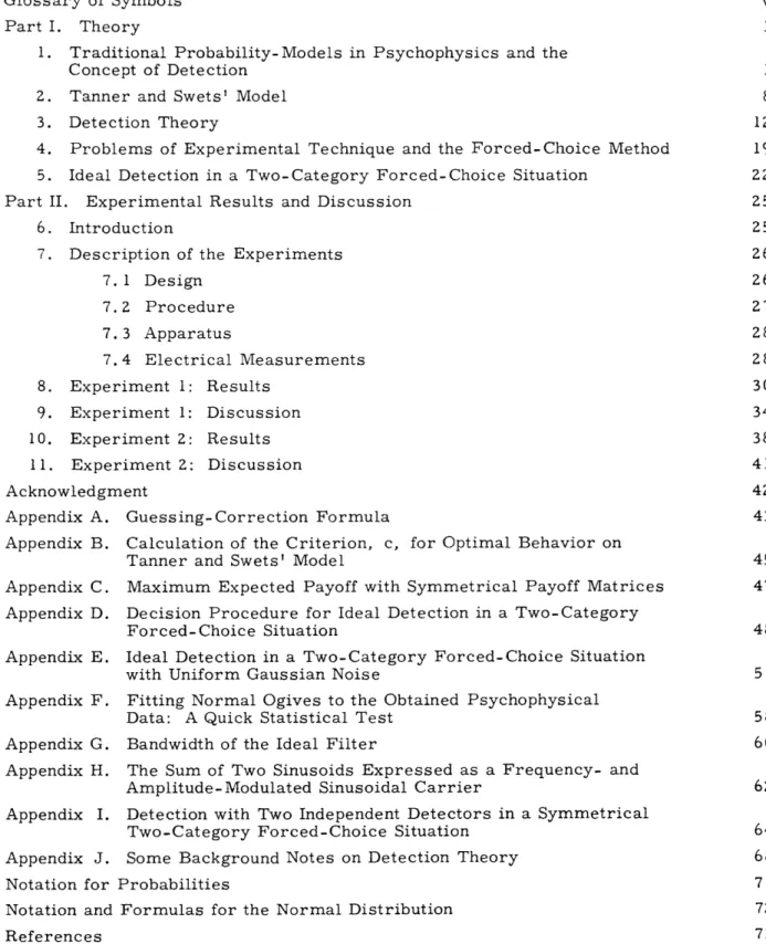
TABLE OF CONTENTS
Glossary of Symbols Part I. Theory
1. Traditional Probability-Models in Psychophysics and the Concept of Detection
2. Tanner and Swets' Model 3. Detection Theory
4. Problems of Experimental Technique and the Forced-Choice Method 5. Ideal Detection in a Two-Category Forced-Choice Situation
Part II. Experimental Results and Discussion 6. Introduction
7. Description of the Experiments 7. 1 Design 7. 2 Procedure 7.3 Apparatus 7. 4 Electrical Measurements 8. Experiment 1: Results 9. Experiment 1: Discussion 10. Experiment Z: Results 11. Experiment Z: Discussion Acknowledgment Appendix A. Appendix B. Appendix C. Appendix D. Appendix E. Appendix F. Appendix G. Appendix H. Appendix I. Appendix J. Notation for Notation and References Guessing-Correction Formula
Calculation of the Criterion, c, for Optimal Behavior on Tanner and Swets' Model
Maximum Expected Payoff with Symmetrical Payoff Matrices Decision Procedure for Ideal Detection in a Two-Category Forced- Choice Situation
Ideal Detection in a Two-Category Forced-Choice Situation with Uniform Gaussian Noise
Fitting Normal Ogives to the Obtained Psychophysical Data: A Quick Statistical Test
Bandwidth of the Ideal Filter
The Sum of Two Sinusoids Expressed as a Frequency- and Amplitude-Modulated Sinusoidal Carrier
Detection with Two Independent Detectors in a Symmetrical Two-Category Forced-Choice Situation
Some Background Notes on Detection Theory Probabilities
Formulas for the Normal Distribution
iii v 1 1 8 12 19 22 25 25 26 26 27 28 28 30 34 38 41 42 43 45 47 48 51 58 60 62 64 68 71 72 73
_ 1_1 11______1
-·^IIIIIL__-GLOSSARY OF SYMBOLS
A parameter determined by the payoff matrix and the a priori probability of a signal.
c The criterion which must be exceeded by the effective stimulus magnitude for a perception (earlier model) or a response (later model) to occur.
C The momentary threshold.
C (The event of) a correct response. Pr(C), the probability of a correct response, is called the detectability.
d' The effective stimulus magnitude corresponding to a given signal. E The signal energy.
E( ) The expected value of .... E(X) is the mean of the random variable X. exp[ ] The number e raised to the power ...
fN The probability density of the receiver input when noise alone is present.
fSN The probability density of the receiver input when signal and noise are present. FN The (complementary) distribution of the likelihood ratio of the receiver input
when noise alone is present.
FSN The (complementary) distribution of the likelihood ratio of the receiver input when signal and noise are present. Thus FSN(P) is the probability that the likelihood ratio of a receiver input containing both signal and noise exceeds the number p.
L( ) The likelihood ratio. L(T') = fSN(T) /fN( ) No The noise power in a l-cps band.
N[
]
The normal distribution function. (See section on notation and formulas for the normal distribution).P (The event of) a perception. P is the complementary event.
Pr( ) The probability of ... . (See section on notation for probabilities.) Pr(C) The probability of a correct response; the detectability.
'IT The set X',X 2 ... X2TW / may be thought of as an alternative representa-tion of the receiver-input time-funcrepresenta-tion.
Analogously to4T,
4T1
is the receiver input in the first observation-interval of a two-category forced-choice trial.\'1 The receiver input in the second observation-interval of a forced-choice trial. Qi The outcome of a detection trial. The event Q1 Q2'Q 3' or Q4 occurs according
as S R, S R, S R, or S- R occurs.
r The signal-energy to noise-spectrum-level ratio expressed in decibels. R One of the two possible responses in a detection situation. R is the response
that yields the higher payoff in case S obtains. The complementary response is R. (These symbols are not used in the forced-choice situation.)
R1 One of the two possible responses in a two-category forced-choice trial. R1 is the response which yields the higher payoff in case S:S obtains. The com-plementary response is R2.
S One of the two possible states (of stimulation) in a detection situation. Speci-fically, in a yes-no situation in which noise occurs on every trial and a signal occurs on some trials, S is the event that the signal occurs. The
comple-mentary event is S. (These symbols are not used in the forced-choice situa-tion.)
S:S In a two-category forced-choice situation in which noise is presented in both observation-intervals and a signal is presented in only one, S:S is the event that the signal occurs in the first observation-interval. The complementary
event is S:S.
S R The joint event S and R.
T The duration of an observation-interval. Var( ) The variance of ...
Vi The (payoff) value of the event Qi' W The bandwidth of the noise.
.th
X. The value of the receiver-input time-function at the 1 sampling point; a
--1random variable.
random variable.
PART I. THEORY
1. TRADITIONAL PROBABILITY-MODELS IN PSYCHOPHYSICS AND THE CONCEPT
OF DETECTION
We consider a given signal and a given condition under which this signal is presented to a subject. Our aim is to predict the probability that the subject will perceive the
signal.
In order to make predictions we must have a model, and any psychophysical model must come to grips with at least two facts: (a) Subjects exhibit variability of a "random" sort: on some trials the signal is perceived (we shall say the event P occurs), on others the signal is not perceived (the event P occurs), and there is no way - at least no obvious way - of predicting the sequence of the events P and P in a group of trials. (b) The probability that the signal is perceived, Pr(P), increases as the signal magni-tude increases, other things being equal.
The model to account for these facts is sometimes constructed as follows. Whether P or P occurs on a given trial, it is argued, depends on the value assumed on that trial by some variable quantity within the subject. Let us call this quantity "the effec-tive stimulus magnitude" and designate it by d'. (This symbol is taken from Tanner and Swets (21) and introduced here in anticipation of our discussion of their model.) If on a given trial d' exceeds some cutoff value c, then P occurs; otherwise P occurs. That is, the signal must generate within the subject an effective stimulus magnitude greater than some minimum quantity in order to be perceived.
Next we must introduce some random variability and also bring the signal magnitude into the picture. Several approaches can be taken. We shall discuss two.
Threshold Approach. In this approach we argue that the quantity c is a random variable (which, in our notation, must be represented by C - with the exception of the
random variable ', all random variables will be designated by underlined capital letters). On a given trial, C assumes a certain value, which might be called the "true momentary threshold" for that trial. C will vary from trial to trial in some irregular fashion as a result, presumably, of some random variability in the subject.
The quantity d', on the other hand, is conceived of as a simple function of the signal magnitude. To each signal magnitude there corresponds an effective stimulus magnitude, the latter being presumably a nondecreasing function of the former.
It is frequently hypothesized [the "phi-gamma hypothesis" (7)] that the random vari-able C has a normal, or gaussian, distribution. In this case we have (see the sections on Notation for Probabilities and on Notation and Formulas for the Normal Distribution):
Pr(C<x) = N [x; E(C), Var(C)] (1.1)
The basic statement of the model - that the quantity C must be exceeded by the effec-[. tive stimulus magnitude for perception to occur - may be written
I 1
Pr(P) = Pr(C < d' )
From Eqs. 1.1 and 1.2 we get
Pr(P) = N [d'; E(C), Var(C)1 (1.3)
which is the "psychophysical function" according to the present model. That is, it is the function that relates the probability of perception to the signal magnitude, or, as in the present case, to a function of the signal magnitude.
Let us examine the significance of this result. We notice, first of all, that in order to calculate Pr(P) we need to specify two unknown parameters, E(C), the expected true momentary threshold (referred to as "the threshold"), and Var(C), the variance of the true momentary threshold.
What is more unfortunate, however, is that even knowing these two parameters, we still cannot predict Pr(P) from a knowledge of the signal. This is because the independ-ent variable d' of Eq. 1.3 is not a measure of the signal, but of the effective stimulus, and we do not know a priori what signals go with what effective stimuli. What we would have to do is to "scale" the signal magnitudes. That is, we would have to find the rela-tion between some specific measure of signal magnitude (if the signals are tones, such
a measure could be the sound pressure in dynes per square centimeter at the eardrum) and the corresponding effective stimulus magnitude. Having obtained this scale, we could then go from a particular signal to the corresponding effective stimulus, and, by means of the model, predict Pr(P).
Unless, however, this scale can be defined independently of the model, or unless the model is to be used for purposes other than predicting the psychophysical function, such a procedure would be trivial. For we would be using the model, in conjunction with the results of psychophysical experiments, to set up the scale, and then using this
scale, in conjunction with the model, to predict the results of the psychophysical experi-ments.
A second way of deriving the psychophysical function might be called the criterion approach.
Criterion Approach. Here again we have a certain stimulus magnitude d' corre-sponding to a given signal. The effect of the subject's variability is, in the present case, to perturb, not the momentary threshold, but rather the quantity d' itself. If H is a random variable that assumes a value on each trial, and d' is the effective stimulus magnitude that would obtain in the absence of subject variability, then the total effec-tive stimulus magnitude on a trial can be represented by d' + H. The quantity H, it is assumed, has a normal distribution, with the proviso, moreover, that H augments d' as often as it diminishes it; or, in other words, that E(H) = 0. We have, therefore,
Pr(H<x) = N [x; 0, Var(H)1 (1.4)
Again we argue that in order for P to occur on a given trial the (total) effective stimulus magnitude on that trial, d' + H, must exceed a minimum quantity c. Here, this quantity
c is not a random variable but a parameter of the situation, and is called "the subject's criterion.' We have, therefore,
Pr(P) = Pr(d' + H>c) (1.5)
From Eqs. 1.4 and 1.5 we easily obtain the psychophysical function
Pr(P) = N [d'; c, Var(H)] (1.6)
Essentially, this result differs from that obtained with the threshold approach (Eq. 1.3) only in notation. Equations 1.3 and 1.6 both mean that the psychophysical function is a normal ogive when plotted on the scale of d', the scale of effective stimulus magnitudes. Since E(C), Var(C), c, and Var(H) are unknown constants, we can equally well repre-sent either equation simply by
2 Pr(P) = N [d'; ., -]
The results of the threshold and criterion approaches are thus mathematically indistin-guishable, and our earlier comments about the former apply equally well to the latter.
The criterion approach, however, is suggestive of further developments which would seem artificial in terms of the threshold approach. In the first place, we easily obtain an extension of the model for the case in which the signal is not resented on a trial.
--- -_ ____ --- ____ ____ --- ____ d -- --- I-_ - _-_ -_
Our earlier result, Eq. 1.6, was
Pr(PIS) = N [d'; c, Var(H)] (1.7a)
in which we write Pr(P S) to indicate that the function applies only to trials on which the signal is presented. [See the section on Notation for Probabilities.] The case in which no signal is presented is, one might argue, identical with the case given above, with the exception that d' now has a lower value. Since we measure d' on an unknown abstract
scale, it is reasonable to let this lower value arbitrarily be zero. Then we write
Pr(PIS) = N [0; c, Var(H)1 (1.7b)
~I
for trials on which the signal is not presented.... - _- - - - J.-_ -- __ ^- L -1 - --
-i secon avantage o me criIerion approacn lles Ine namiies assgnieu L vU-ouULi
quantities. In the threshold approach, Eq. 1.3, the "central-tendency" term, E(C), was called "the threshold." We are tempted to think of a "physiological" quantity which
is constant, as physiological quantities presumably are, under a wide range of possible psychophysical experiments. In the criterion approach, the central-tendency term, c, is called "the subject's criterion." This suggests a "psychological" quantity which may, as psychological quantities sometimes do, change its value from psychophysical experi-ment to experiexperi-ment. It may even be that the quantity c is somehow correlated with the quantity d'. If this were true, the present model would be in serious trouble. The model is weak to begin with, but it can at least predict the shape of the psychophysical function plotted on the effective stimulus scale. If the correlation being considered existed, the model would not even be able to do that much without knowing the nature of
the correlation. In the criterion approach we are forced to take this possibility more seriously.
Rather than turning to a discussion of this problem of the shifting criterion, we con-sider a more immediate objection. We have begun by considering the prediction of the event P, a perception of the signal. If, however, we have occasion to act as subject in a threshold experiment, we discover that the present "experience model" does not account for our actual experience. According to the experience model the event P occurs whenever the total effective stimulus magnitude exceeds the criterion c; we are tempted to think of a lamp inside the mind which either does or does not light up on a given trial. Our actual experience, however, is not like that; it does not come so neatly dichotomized. This fact, has, of course, long been realized, as is evidenced by the extensive discussion in the psychophysical literature of the problem of guessing (see refs. 1, 7, 21, and our Appendix A, in which the traditional "guessing-correction formula" is discussed). By "a guess" is presumably meant the act of responding "yes, I perceive the signal" when one does not perceive the signal, or at any rate when one is not certain whether or not he does. Now, if experience did come in the dichotomized fashion demanded by the experience model, a well-intentioned subject would obviously find no occasion for guessing. He would simply report whether or not P occurred. Theorists who believe that well-intentioned subjects guess thereby also believe that the experience model does not fit the facts.
There exist, fortunately, events in this situation which do come in the dichotomized fashion predicted by the model. These are the event R of responding "yes, I perceive the signal" and the complementary event R. (Indeed, any two mutually exclusive events whose occurrence is under the subject's control would do.) We can, it will be seen, get out of our present predicament if we modify our model to predict the occurrence, not of P, but of R. Such a "response model," then, asserts that a response R is made when-ever the total effective stimulus magnitude on a given trial exceeds the criterion, leaving questions of experience altogether out of the discussion. While this seems to take us away from traditional psychophysics, it does have the advantage of solving at this stage a further problem that we would sooner or later have had to face: the event P is, for scientific purposes, an unobservable event. To get into the realm of observables, we would have had to make additional assumptions to enable us to predict the occurrence of observable events, such as R, from the unobservable one, P. The response model does not need these additional assumptions. The questions relating to guessing which have bothered workers in this area need, moreover, no longer arise on the response model, since the experience of the subject is now irrelevant.
The response model, then, predicts directly from stimuli to responses, attaining thereby an objective character. There is, unfortunately, one further hitch. What task are we to assign the subject? Presumably we wish to instruct him to respond if and only if he perceives the signal. This is an unpleasant situation, though, for we now find that having deleted mention of experience from the model, it creeps back in the
instructions. The model and the instructions under which the model applies thus bear no relation, at least on this point, to each other. If it were not for the fact that there is a way out of this difficulty - and one that will, moreover, prove helpful in handling the problem of the shifting criterion - we would be tempted here to revert to the
experi-ence model.
We extricate ourselves by the introduction into the experiment of catch-trials, i.e., trials on which the signal is not presented. Once such trials are introduced, a new mode of instruction becomes quite natural: we instruct the subject to try to be correct as often as possible; by "correct" we mean making a response R when there is a signal or making the complementary response R when there is no signal. Or, to make the situation even more general, we may assign values to the various outcomes of a trial. The subject's task is then to maximize the values which accrue to him as a result of such trials. (The term "value" is used in the sense in which it is said that gold has greater value than silver.)
The introduction of catch-trials is, of course, nothing new to psychophysics. What is relatively new, perhaps, is the realization that introducing them brings the psycho-physical experiment under the rubric of detection, thereby rendering psychopsycho-physical problems amenable to analysis in terms of the concepts and results of detection theory. In order to understand this, let us examine in a general way what we mean by a detec-tion situadetec-tion.
Many different formulations are possible. In this report we shall use the concept exclusively in accordance with the following definition.
Definition of the Detection Situation
1. On each "trial" one or the other of two mutually exclusive states S or S obtains. The a priori probability Pr(S) of the occurrence of S is assumed to be a fixed given number.
2. On each trial the subject (the "detector") brings about the occurrence of one or the other of two mutually exclusive events ("responses") R or R.
3. Event Q1,Q 2 Q3' or Q4 occurs on a given trial according as the joint event
S-R, SR, SR, or S-R also occurs on that trial.
4. The occurrence of the event Qi (i = 1, . .. ,4) has a specifiable value, vi (the "payoff value" or "payoff") for the subject. ("Value" is used in the sense defined above.)
5. The following inequalities hold: v > v3; v4 > v2.
Example: A Discrimination Experiment. A rat is placed on a jumping-stand. Facing it across a gap are two cards, one bearing a circle, the other a triangle. An air blast forces the rat to jump at one of the two cards on each trial. The system is so arranged that if the rat jumps at the circle, the card folds back and the rat goes through to find food (the rat is "reinforced"). If it jumps at the triangle, it finds that it cannot go through, bumps its nose, and falls into a net (it is "punished"). On each trial, then, the rat jumps either to the right (R) or left (R). The card bearing the circle is either on the right (S) or left (S). If it is on the right and the rat jumps to the right (S R), the rat
5
II--·-is reinforced on the right (Q1). If the circle is on the left and the rat jumps to the right (S-R), the rat is punished on the right (Q2). If the circle is on the right and the rat jumps to the left (S R), the rat is punished on the left (Q3). And, lastly, if the circle is on the left and the rat jumps to the left (SR), the rat is reinforced on the left (Q4). We assume that being reinforced has a greater value for the rat than being punished, so that vl, the value of the occurrence of Q1, is greater than v3, the value of the occurrence of Q3; likewise v4 is greater than v2.
Remark 1. On occasion we shall refer to certain mechanical devices as "detectors." This is a loose way of speaking, since, presumably, the occurrence of events can be said to have value only to organisms. Strictly speaking, it is the person who uses such a mechanical device who is doing the detecting; it is for him that Qi has value vi .
Remark 2. We shall arrange the payoff values in a payoff matrix: S S
R
R
Remark 3. Clause 5 of the definition, included primarily for subsequent ease of exposition, is not as restrictive as might at first appear. What it does is to rule out two classes of situations. (a) It rules out degenerate situations exemplified by the following payoff matrix:
S S R 1 Z R -3 1
Consider what happens in this situation: If S obtains, response R is preferable, since R yields a larger payoff than R; if S obtains, response R is again preferable for the same reason. Optimal behavior would therefore consist in making response R on every trial without regard to whether S or S obtained. Such situations are clearly of little practical interest. (b) Clause 5 excludes situations that differ from the included ones only trivially in notation, as, for instance,
S S R -1 1
If in this matrix we replace S by S and S by S, we obtain a matrix that satifies the inequalities of clause 5. Excluding such "mirror image" cases enables us to state very simply what we mean by the accuracy of detection.
Accuracy of Detection. To make response R when S obtains - this is sometimes called a "hit" - or to make response R when S obtains is, we shall say, to make a correct response. To make response R when S obtains - this is sometimes called a "false alarm" or to make response R when S obtains sometimes called a "miss" -is to make an incorrect response. The accuracy of detection in a given situation will, of course, be measured by the ratio of the number of correct responses to the total number of responses made in the situation.
If in a given situation the accuracy of detection is ao, we shall say that the detec-tability of the signal (to be defined later) in that situation is a .
Expected Payoff. If we know the probability of a hit, Pr(RIS), and the probability of a false alarm, Pr(RIS), in a given situation, we can calculate the expected value of the payoff according to the following obvious formula:
E(V) = v1Pr(R IS) Pr(S) + v2Pr(R S) Pr(S)
+ v3Pr(R IS) Pr(S) + v4Pr(R S) Pr(S) 8)
2. TANNER AND SWETS' MODEL
In Tanner and Swets' model (19, 20, 21), the prototype of the psychophysical experi-ment is the detection situation defined in the previous section (with the event S being the occurrence of some signal). The mathematics of the model, however, is still for the most part that of traditional psychophysics. Indeed, the psychophysical function is assumed to be given by our Eqs. 1. 7, with the additional statement that Var(H) = 1. The important assumption behind this statement is that the variance of H is independent of the various other parameters of the situation. Picking the value unity is of no particular significance, since the scale on which H is measured is still arbitrary: letting
Var(H) = 1 amounts to picking a unit of measurement on this scale. Since we are dealing with a response model, we shall also change the equations to the extent of writing R where we previously wrote P. Equations 1. 7a and 1. 7b become
Pr(R| S) = N[d'; c, 1 (2. la)
Pr(RS) = N[ 0; c, 11 (2. lb)
The reader will recall how these equations were obtained. On each trial there is assumed to exist an effective stimulus of total magnitude d' + H, where H is a normally distributed random variable with mean zero. The quantity d' is assumed to be a (non-decreasing) function of the signal magnitude, so that d' + H will, on the average, be
large or small, according as the signal is strong or weak. If no signal is presented, d' is assumed to have the value zero. Response R occurs on a given trial if d' + H > c on that trial, c being a criterion set by the subject.
From Eq. 2. lb we see that Pr(RIS), the probability of a false alarm, is a function solely of the criterion c. If the subject sets his criterion to a low value, i.e., one that will frequently be exceeded by d' + H. the false alarm rate will be high; if he sets the
criterion high, the false alarm rate will be low. Conversely, the false alarm rate determines the criterion; measuring the former in an experiment enables us by Eq. 2.lb to calculate the latter.
The experiment in which we measure the false alarm rate can also, of course, yield a measure of Pr(RIS), the probability of a hit. The measured probability of a hit,
together with the calculated value of c, can then be introduced into Eq. 2. la, and this equation solved for d'.
The whole process can then be repeated with a different signal magnitude. For each signal used we measure Pr(RIS) and Pr(R S); these two quantities in turn yield a value of d'. We have thus constructed a scaling procedure, i. e., a procedure that enables us to determine d' for any given signal.
We could check on this procedure in the following manner. First we set up a detec-tion situadetec-tion s1 by specifying a given signal, payoff matrix, and a priori probability Pr(S). In situation s we measure Prl(RIS) and Prl(RIS) . Then we set up situation s2 with the same signal but with a different payoff matrix and/or Pr(S). Our psychophysical
measurements now yield Prz(R S) and Pr(RIS). Since s1 and s2 are different situations, we find, presumably, that Pr 1(RIS) * Pr2(RIS) and that Prl(R S) Pr 2 (R S). For a
subject behaving optimally, at any rate, these inequalities can be shown to hold. We now solve Eqs. 2.1, using Prl(R S) and Prl(R S), and obtain a value d' . Repeating the process, using Pr2 (R S) and Pr2(R S), we obtain d'. Under ideal circumstances,
i. e., if there is no experimental error, we should find that d' 1 = d'2' since both of these numbers measure the effective stimulus magnitude of the same signal. Unfortunately, we would need further statistical analysis to determine what discrepancies we could tolerate, and such an analysis has not, to our knowledge, been developed.
Tanner and Swets' model enables us to relate our uncertainties one to the other. We can, for example, write the probability of a hit as a function of d' and the
probabil-ity of a false alarm, eliminating the criterion c. The predictive power per se of the model is not, however, increased thereby. If our interest lies in predicting the psy-chophysical function, i.e., in predicting the probabilities Pr(RIS) and Pr(RjS) corres-ponding to a given signal, we still have to know beforehand: (a) the magnitude of our signal on the effective stimulus scale; and (b) the value of the parameter c. From the point of view of experimental prediction we have improved on the venerable phi-gamma hypothesis only to the extent of writing Eq. 2. lb; that is, only to the extent of adopting the criterion approach of the last section.
We now want to gain some insight into how we can change the false alarm rate with-out changing the signal. It is essential that we be able to do so in order to have a check on the scaling procedure just described. Consider the following example.
Example. Let the payoff matrix be
S S
R 100 0
R 0 1
and let Pr(S) = 0.99. In such a situation a clever subject will almost always make the response R, since if he makes this response he stands a good chance - indeed a 99 to 1 chance -of being paid 100; but if he makes response R, he can at most be paid 1 - and that much only once in a hundred times. The subject will therefore, presumably, set his criterion very low so that it will almost always be exceeded by d' + H, and response
This concept is defined below. In order for the inequalities to hold, it is sufficient (in optimal behavior) for the parameter , defined by Eq. 2. 2, to assume different values in situations s and s2.
Tanner and Swets also show how predictions in the present kind of psychophysical experiment are related to predictions in the "forced-choice" experiment. This part of their model will not be discussed. The forced-choice situation in general will be dis-cussed in sections 4 and 5.
9
R will be made on almost every trial. Only if the total effective stimulus magnitude is extremely low will he let himself be convinced that the signal was not presented (that d'
= 0 on that trial) and make response R.
If we change the situation by letting the payoff matrix be
S S
R 1 0
R 0 100
and by letting Pr(S) = 0. 01, the reverse will presumably occur. The subject will now set his criterion very high and make response R on almost every trial. Only if the effective stimulus is extremely large, will he take it as evidence that a signal was pre-sented (that d' 0 on that trial) and make response R.
We see, therefore, that a clever subject will pick his criterion differently in dif-ferent situations even though the signal remains the same. We might even suspect that there is an optimal way of picking the criterion so that the expected payoff to the subject is maximized in the given situation. A subject who sets his criterion to such an opti-mal value, cmax, would be said to be behaving optimally.
[A subject behaving optimally in the sense of the present discussion must not be confused with what we shall call an ideal detector. The latter maximizes the expected value of the payoff. The former maximizes the expected value of the payoff in a situa-tion in which condisitua-tions (1.4) and (1. 5) - the fundamental condisitua-tions of the model - hold. We may say that our optimally-behaving subject is an ideal detector for a situation in
which the information about the signal and the variability ("noise") is available only in the form stipulated by Tanner and Swets' model.]
While Tanner and Swets themselves do not particularly stress this notion of optimal behavior, it might be of interest here to investigate it somewhat further. The mathe-matics of the situation is worked out in Appendix B. Here we merely state the result. First, a definition:
(v4 - v2) Pr(S)
Let = (v-1 - v3 ) Pr(S) (2.2)
This quantity incorporates the relevant information about the payoff matrix and the a priori probability of a signal. In terms of the (known) parameter we find that
In d' (2. 3)
max 2
d'
Putting this result in Eqs. 2. 1 and rearranging terms, we see that for a subject behaving optimally the psychophysical function is
d'
Pr(R 1
NL0,2
(Z.4a)In
p
Pr(R S)= 1- N + 0, 1 (2. 4b)
Note that these functions (plotting the probability versus d') are not, in general, in the shape of normal distributions (normal ogives are obtained only in case = 1). This may be considered startling when we reflect that our basic equations (2. 1) are, of course, normal ogives. The difference occurs because the subject behaving optimally changes his criterion not only with changes in the payoff matrix or the a priori probability but also with changes in the signal (changes in d'). Thus, the quantities c and d' appearing in Eqs. 2. 1 are not independent of each other in the case of optimal behavior; insofar as our subjects approximate such optimal behavior the usefulness of these equations may therefore be seriously doubted even if the model that led to them is accepted.
In our discussion of the scaling procedure we saw that the two measured probabilities Pr(R S) and Pr(R S) corresponding to a given signal were necessary to yield an estimate of d'. We see from Eq. 2.4 that on the assumption of optimal behavior each of these two probabilities yields an estimate of d'. This provides us with a check for optimal behav-ior: The experimenter selects a value of , that is, selects a payoff matrix and a Pr(S), and selects a particular signal to be used. The probability of a hit and of a false alarm are then measured. Each of these yields an estimate of d'. The two estimates ought to agree within the tolerance of experimental error if the subject is behaving optimally (some statistics would again be necessary to determine this tolerance). Unfortunately, the experiment performed by Tanner and Swets did not follow this straightforward pro-cedure. Their experiment - which according to our definition is not a detection situa-tion - was set up so that on each trial there was presented either no signal or one of four signals differing in magnitude, the payoff matrix being
S1 S2 S3 S4 S
R
R
It is not clear to us how, fromr whether or not the subject was
the results of such an experiment, one could determine behaving optimally.
11
V1 v1 v1 v1 V2
3. DETECTION THEORY
[The material for this section is drawn from Peterson and Birdsall (15). The reader is referred to their monograph for further details, proofs, and a short bibliography of other writings on detection theory. A brief historical introduction to detection theory is given in our Appendix J.]
In discussing the models considered thus far we spoke of signals in a very general way. The specific nature of the signal - its duration, for instance - played no part in the theorizing. Likewise, the nature of the random variability was hardly analyzed: we arbitrarily assumed the existence of a single random variable H with normal distribu-tion and fixed parameters.
A more sophisticated analysis is made in detection theory; it results, as one would expect, in a model of greater power, although, admittedly, also of greater mathematical complexity. It is the purpose of this section to present some of the fundamental ideas of this theory.
The Signal. By a signal, we shall understand a measurable quantity varying in a specified manner during a fixed observation-interval T seconds long. Letting time be measured from the beginning of the observation-interval, we may represent the signal by a time-function s(t) defined on the interval 0 < t < T.
It will be assumed that s(t) is series-bandlimited to a bandwidth W s. By this we mean that s(t) has a Fourier series expansion on the interval 0 < t < T; that the series contains only a finite number of terms; and that the frequency of the highest harmonic
is Ws s
The Noise. As in previous models, we shall assume that the signal is perturbed by random variability. Since the signal is now represented by a time-function, we must let this perturbation occur at each moment of time at which the function is defined. Mathematically we do this by adding to our signal-function s(t) a "random" time-function, i. e., a function whose value at each moment of time is specified only in a statistical sense. Such a function n(t), 0 < t < T, will be said to describe the noise in the situation. It will be assumed that n(t) is series-bandlimited to a bandwidth W > Ws
Receiver Inputs; the Events S and S. Each observation-interval thus yields a time-function. Such a function - or its physical counterpart - is called a receiver input. It is designated by x(t).
By saying that the signal is presented during a given observation-interval, we mean that the receiver input for that interval is given by
x(t) = s(t) + n(t) 0 < t < T
By saying that the signal is not presented during a given observation-interval, we mean that s(t) = 0 for that interval, so that the receiver input is given simply by
x(t) = n(t) 0 < t < T
In either case the receiver input is given by a series -bandlimited time-function defined on the interval 0 < t < T; this function is "random" since, in either case, it contains the "random" term n(t).
The Sampling Theorem. We shall need one form of the so-called sampling theorem in the time-domain. [For a proof of this theorem see Appendix D of reference 15. Also compare references 5 and 16.] The theorem states that any fixed time-function defined on an interval 0 < t < T and series -bandlimited to a bandwidth W can be uniquely repre-sented by a set of 2TW numbers, these numbers being the value of the function at
"sampling points" 1/2W seconds apart on the time-axis.
Accordingly, if we knew the value of x(t) at each of the ZTW sampling points, we could reconstruct x(t). The function x(t), however, is a "random" function; its value at the sampling points is determined only in a statistical sense. Thus, instead of repre-senting this function by ZTW numbers, as we would in the case of an ordinary
well-specified function, we must use, instead, a set of 2TW random variables, X1,X2 .. X2TW On occasion it will be found convenient to denote this set by the single letter Ip".
We have, thus, three equivalent ways of writing a receiver input: x(t); X1 .XZTW and .
Probability Density of the Receiver Input. We consider, next, the joint probability
density of the random variables X1, . . XZTW. (It is here assumed that the density exists, i. e., that the joint distribution function of the Xi has all derivatives.) This density will, by virtue of the sampling theorem, give us the complete statistical speci-fication of the receiver input.
Actually, it will be found convenient to break up this density into two conditional densities, one for each of the two cases S and S. The symbol "fSN" will be used to denote the joint density (of X1, .,X2TW) that obtains in case the receiver input contains both signal and noise; "f N will be used for the density in the alternative case of noise alone.
In formal notation we have
Pr(X1 < a1 , X < a . XZTW < aZTW I S) a1 a aT w _SN (xi, l.Xg ; .. I xZTW) dxldxg ' dxZTw -cc -00 -00 Pr(X1 < a1, X2 < a X2T < aT W S) a 1 a aZTW a1a fN(xl, x, ... , x2T w ) dxldx2... dx2TW
Likelihood Ratio. Recall that the probability density of the receiver input is fsN(xl ... xZTW) or fN(xl ... XW.. ) according as the signal is or is not presented.
We now define the likelihood of the receiver input to be fSN(Xl ... XTWw) or fN(X1 . XZTW) according as the signal is or is not presented. 2 .. In our summary nota-tion, the likelihood is written fSN( ) or fN(T). The likelihood ratio L(4'') of a receiver input is then defined as follows:
fSN ( X ) fsN(X 1 .... .XZTW)
L() fN( ) - fN(Xl ... 2T W)
The likelihood ratio of a particular receiver input tells us, very roughly speaking, how likely it is that this input contains the signal; if the likelihood ratio is large, we may take it as evidence that a signal is present; the larger the likelihood ratio, the weightier the evidence. Since our receiver input is random, we can never, of course, be sure; some receiver inputs containing the signal and noise will yield low values of the likelihood ratio, and some containing only noise will yield high values.
The likelihood ratio must not be confused with the ratio fsN(l ... X2TW)
fN(Xl .. X2TW)
of the densities. The variables occurring in the likelihood ratio, unlike those occurring in the ratio of the densities, are random variables. The likelihood ratio is thus a func-tion of random variables, and, like any funcfunc-tion of random variables, is itself a random variable. It is thus meaningful to speak of the distribution of the likelihood ratio, while it would be nonsensical to speak of the distribution of the ratio of densities, just as it would be nonsensical to speak of the distribution of a distribution.
As in the case of the receiver-input density, we break up the distribution of the likelihood ratio into two conditional distributions, one for each of the two cases S and S. Denoting these distributions* by FSN and FN, we have
FSN(x) = Pr(L(P) > x IS) (3. la)
FN(X) = Pr(L(I/) > x S) (3. lb)
Thus, the expression FSN(D), to be used later, designates the probability that the likeli-hood ratio of a receiver input containing the signal exceeds the number . The expres-sion FN(P) designates the corresponding probability for a receiver input containing noise alone.
To fix our ideas, let us consider the following simple example.
Example: Likelihood Ratio in a Discrete Case. We are given a loaded coin, and we know, for one reason or another, that the odds are 10 to 1 in favor of a particular one of the two faces coming up when the coin is tossed, but we do not know which face
Notice the direction of the inequality in Eqs. 3. la and 3. lb. The functions are complementary distribution functions, since they give the probability that L(4I) lies between x and +oo, rather than between -co and x, as is usual.
is favored. We decide to toss the coin once and count the number K (O or 1) of "heads" that come up. K is our receiver input. We shall say that the event S or S obtains according as the true probability of heads is 1/11 or 10/11.
Since we are dealing with discrete quantities, we shall write probability distributions rather than densities. Thus,
fsN(n) = Pr(K = nIS) = (1/1 1)n (1 0/1 1)1-n (3. a)
fN(n) = Pr(K = n S)= (1 0/11)n (1/1 1)1n (3. 2b)
(n = 0 or 1)
The likelihood ratio is
fsN(K) (1/1 ) (10/) 1-2
L(K) = = 10 -K (K = 0 or 1)
fN(K) )K 1-K
The likelihood ratio is thus seen to be a simple function of the random variable K. It is itself a random variable and has a probability distribution. Let us calculate this distribution for the case in which S obtains; that is, let us calculate
Pr(L(K) = mlS) = Pr(10l2K = mIS) (m = 1/10 or 10)
Replacing the expression 1 0l K - m by the equivalent expression K = (1 - log m)/2, we have
Pr(L(K) = mlS) = Pr = og m 2
Replacing n in Eq. 3. 2a by (1 - log m)/2 we obtain our result 1-log m 1-log m
Pr(L(K) = mIS) = (1/11) 2 (10/11) 2 (m = 1/10 or 10)
By a similar argument we can obtain
1-log m 1-log m
Pr(L(K) = m|S) = (10/11) 2 (1/11) 2
We see, therefore, that the random variable L(K) assumes the values 1/10 and 10, respectively, with probabilities 1/1 1 and 10/11 if S obtains, and with probabilities
10/11 and 1/11 if S obtains.
A Fundamental Theorem of Detection Theory. Consider a detection situation as
defined in section 1, with given payoff matrix and Pr(S), and with the event S defined to be the occurrence of a given signal; and consider the following Decision Procedure: For any receiver input make response R if and only if L(T ) > p, where is given by Eq. 2.2.
15
Theorem. A detector behaving in accordance with the decision procedure maxi-mizes the expected value of the payoff in the given detection situation. Conversely, a detector maximizing the expected value of the payoff in the given detection situation makes the same responses as one behaving in accordance with the decision procedure.
[For proof, see Peterson and Birdsall's Theorems 1 and 2, section 2.4. 2 (ref. 15).] A detector behaving in accordance with the decision procedure will be called "an ideal detector". For an ideal detector we see that
Pr(R!S) = Pr(L(/) > IS) = FSN( ) (3. 3a)
Pr(R S) = Pr(L(4) > S) = FN(O) (3. 3b)
Continuation of the Preceding Example. Suppose that on the basis of our toss of the coin, i. e., on the basis of K, we are required to choose between response R and R. Suppose, moreover, that we are given that Pr(S), the probability that the coin is biased toward tails, is 1/12, and that the payoff matrix is
S S
R 1 -1
R -1 1
With this payoff matrix and this value of Pr(S) we find that = 11, and the fundamental theorem tells us to make response R if and only if L(K) > 11. In the present example,
however, the likelihood ratio never exceeds 10, as we have already seen. Thus, Pr(R IS) = Pr(R S) = 0. The expected value of the payoff in this case is 10/12 = 0. 82, as may be established by substitution into Eq. 1. 8.
Suppose that we pick a decision procedure not in accordance with the fundamental theorem. Thus, for example, suppose that we decide to make response R if and only
if L(K) > 1. We have already calculated that the probability of this event is 10/11 in case S obtains, and 1/11 in case S obtains. Thus, Pr(RIS) = 10/11 and Pr(RIS) = 1/11. Putting these values into Eq. 1. 8 we find that the expected value of the payoff is now reduced to 49/66 = 0. 74.
We thus see that in ideal detection the critical quantities are the distribution func
-tions FSN and FN of the likelihood ratio of the receiver input. Fortunately, Peterson and Birdsall (15) have calculated these functions for a wide variety of signals presented in uniform gaussian noise. We can introduce their results directly into Eq. 3. 3 to
*
By a uniform gaussian noise we mean a time-function whose distribution of instantaneous amplitudes is gaussian (normal) and whose power-spectrum is uniform over a given range and zero outside that range.
obtain the psychophysical function for the ideal detector. If the signal is known exactly, as it would be with a pure tone of known amplitude, frequency, and phase, we obtain
Pr(R S) = 1 - N - d- 0, (3.4a) Pr(R IS) = 1 - N0 + ; 0, (3.4b) where 2 ZE d = N ' E
being the signal energy (the signal power multiplied by T), and
E being the signal energy (the signal power multiplied by T), and No being the noise
power per unit bandwidth (cps).
We notice, incidentally, that if we write d' for d in the expressions above, we obtain Eqs. 2.4, which, it will be recalled, hold for the case of optimal behavior on Tanner and Swets' model. The difference is that in the present equations the variable d is measured
in actual physical units, while in Tanner and Swets' situation the variable d' is measured on an unknown scale of effective stimulus magnitudes. It may be added, parenthetically, that if we had chosen a somewhat different situation - for example, one in which the
signal had unknown phase - we would have obtained an entirely different set of functions for Pr(R S) and Pr(R S).
The two probabilities Pr(R IS) and Pr(R IS) may, of course, be combined into a single quantity, the probability Pr(C) of a correct response, or detectability, as defined in section 1. The formula for doing so is, obviously,
Pr(C) = Pr(RIS) Pr(S) + Pr(RIS) Pr(S) (3.5)
The detectability function for the case of the signal known exactly may be found by sub-stituting the expressions for Pr(RIS) and Pr(RIS) from Eqs. 3.4 in Eq. 3.5. The resulting function with Pr(S) set to 1/2 is plotted in Fig. 1 for several values of p.
We have seen in a general way how the ideal-detector psychophysical function for a particular kind of signal and of noise can be obtained. Let us examine this result. It has already been remarked that, in the present case, unlike that of optimal behavior on Tanner and Swets' model, there is no uncertainty about scales. We notice, moreover, that the effect of changing the duration of the signal is immediately given by Eqs. 3.4. For instance, we see that increasing the signal duration and decreasing the signal power by a given factor leaves everything unchanged. This is the so-called I-T Law of psycho-physics, which is found to hold within limits (11). The equations also predict constant detectability for constant signal-to-noise ratio, other things being equal; this, too is found to hold within limits in auditory experimentation (11). Furthermore, the equations show that for an ideal detector the detectability is independent of the noise bandwidth; auditory experiments reveal that this is the case for human subjects, again within limits (11).
17
r*r)p-1.0 0.9 0.8 J 0.7 ao w 0.6 0.5 Pr (S)-0.04 0.06 0.1 0.2 0.4 0.6 1 2 4 6 10 20 E/No
Fig. 1. Ideal-detector psychophysical functions. Signal known exactly; Pr(S) = 1/2. ("Yes-No' situation.)
Aside from these (perhaps accidental) facts, we might ask what relevance this kind of model has, in general, to empirical psychophysics, knowing, as we do in advance, that no subject is an ideal detector. First of all, the model allows us to place lower bounds on our threshold measurements. For example, we see from Fig. 1 that for a signal known exactly, a uniform gaussian noise, and Pr(S) = 1/2, the detectability can-not exceed 0. 76 if the signal energy does can-not exceed the noise power per unit bandwidth. In similar fashion, lower bounds can be set for a wide variety of situations. Second, establishing the manner in which and the extent to which a subject's behavior differs from that of an ideal detector might lead to interesting insights into sensory psychology. If, moreover, the difference between subject and ideal detector is found to be expressible in terms that are sufficiently simple, we might be able to generate, by simple additions to the present model, a powerful tool for the prediction of actual behavior.
4. PROBLEMS OF EXPERIMENTAL TECHNIQUE AND THE FORCED-CHOICE METHOD
A basic problem concerning the payoff matrix has thus far been avoided. Recall that the vi are the values, for the subject, of various events in the detection situation. How are we to determine these values ? To be sure, the experimenter may try to assign the values by using a system of monetary rewards and fines. There is no guarantee, however, that the value for the subject corresponds to the number of cents involved; the value of two cents may be different from twice the value of one cent.
Moreover, the various events in the detection situation may have "private" values for the subject, prior to or independently of the assignment of values by the experimenter.
Thus, in a particular experiment we might have:
Q2: subject is fined $1 upon making response R when S obtains (i.e., upon making a false alarm);
Q3: subject is fined $1 upon making response R when S obtains (i.e., upon missing the signal).
Even though the money involved in Q2 and Q3 is the same, the amount of displeasure experienced by the subject may be quite different in the two cases. If Q3 occurs, the subject may reflect that he has made response R (which is appropriate to trials on which there is no signal, since in that case it earns $1) on a trial on which there was a signal; but after all, no one is perfect, the signal was very weak, etc., ... On the other hand, if Q2 occurs, he may reflect that he has made response R (appropriate to trials
on which there is a signal) on a trial on which there was no signal; the experimenter may think he is having hallucinations, perhaps there is something wrong with his sense organs, etc .... If the subject has such feelings, the values of Q2 and Q3 will be quite
different.
It would be excellent, therefore, if we could get along without the v. altogether.1 This we cannot do. We can, however, take a step in that direction with the help of the following result.
It is easy to show (see Appendix C) that the maximum expected payoff is independ-ent of the v. so long as
1
v1 = V4 and v2 = v3 (4. 1)
A payoff matrix for which Eq. 4. 1 holds will be called symmetrical.
Thus, if a subject is instructed to try to maximize the values that accrue to him, his task, and therefore presumably his behavior, will be independent of the payoff
matrix, so long as the latter is symmetrical. Instead of having to worry about four quantities, therefore, we need worry only about the symmetry of the payoff matrix.
*
Strictly speaking, these instructions are unnecessary, since what we presumably mean by "value" is "something which people try to maximize."
19
__I^I___I___IIIIYL_·I-PI1·-L·--As our discussion has just shown, however, the kind of experimental situation we have been considering is basically asymmetrical: Q2 and Q3- or Q1 and Q4, for that
matter - are psychologically different and may therefore have intrinsically different values for the subject. It is felt that condition (4. 1), if not totally satisfied, can at least be approximated better in an experiment using the so-called (temporal) two-category forced-choice technique.
The experimental technique implicit in our discussion thus far has been the :'yes-no" method. We are using this method whenever we set up our experiment as a detection situation in accordance with the definition of section 1, interpreting the event S of that definition to be the occurrence of a signal (as defined in section 3). Thus, on each trial of a yes-no experiment there is an observation-interval during which the signal may occur.
In the two-category forced-choice method there are on each trial two observation-intervals, during one and only one of which the signal occurs (whether on a given trial the signal occurs during the first or second observation-interval is determined, of course, at random); the noise (if any) occurs in both observation-intervals. Otherwise the forced-choice and the yes-no experiments are identical.
The forced-choice situation, it will be observed, fits our definition of a detection situation if we interpret the event S of that definition to be the occurrence of a signal in the first observation-interval (with the event S consequently to be interpreted as the occurrence of a signal in the second observation-interval).
In order for the notation to be indicative of the kind of experiment being discussed, the symbols S, S, R, and R, will be reserved for the yes-no situation, and the symbols S:S (signal in the first interval, no signal in the second), S:S, R1, and R2 will be used for the corresponding events in the forced-choice situation.
The objectional kind of asymmetry found in the yes-no technique is not present to such an extent in the forced-choice technique. We may set up the following forced-choice situation, where, to emphasize the symmetry, we let the subject indicate his responses by pushing a switch to the left or right:
Q1: subject is paid D dollars upon receiving the signal in the earlier
observation-interval and pushing the switch to the left;
Q2: subject is fined D' dollars upon receiving the signal in the later interval and pushing the switch to the left;
Q3: subject is fined D' dollars upon receiving the signal in the earlier interval and
pushing the switch to the right;
Q4: subject is paid D dollars upon receiving the signal in the later interval and
pushing the switch to the right.
Except for an interchange of "earlier" with "later" and of "left" with "right," our descriptions of Q1 and Q4, and of Q2 and Q3, are identical. In order for Eq. 4. 1 to hold, therefore, we need only assume that such temporal and spatial differences do not
affect the values that the subject places on the events.
If this assumption is true, i. e., if the value of Q1 equals that of Q and the value of Q2 equals that of Q3, then our previous result tells us that it is immaterial what the actual values are. For that matter, the monetary values D and D assigned by the experimenter are also immaterial; we may replace the event of being paid D dollars by a flash of green light, for example, and the event of being fined D' dollars by a flash of red light, with the understanding that the green light is "correct" or 'good,;' while the red light is "incorrect" or bad.l Our instructions to the subject may then simply be to try to maximize the occurrence of flashes of the green light.
In order to complete the symmetry of the situation we may want to set
Pr(S:S) = Pr(S:S) = 1/2 (4. 2)
A forced-choice situation in which both Eqs. 4.1 and 4.2 hold will be called a"symmet-rical forced-choice situation. T
21
5. IDEAL DETECTION IN A TWO-CATEGORY FORCED-CHOICE SITUATION Let us consider a signal s(t) and a noise n(t), as defined in section 3. Since we are dealing with a forced-choice situation, we shall have two observation-intervals and, hence, two receiver inputs, xl(t) and x2(t). If xl(t) = s(t) + n(t) and x2(t) = n(t), we say that S;S obtains; if xl(t) = n(t) and x2(t) = s(t) + n(t), we say that S:S obtains. Either S:S or S:S must, of course, obtain on a given trial.
We have already seen how a receiver input may be considered to be a set ' of 2TW random variables. Two such sets, ' 1 and , will be necessary here, to correspond to the two receiver inputs xl(t) and x2(t). Notice that on any given trial one of the two quantities, 1 I2' has the density fSN and the other the density fN'
The payoff matrix for the forced-choice situation is written S:S S:S
R1 R2
where v1 > v3, and v4 > v2. Corresponding to our earlier definition, we have
(v4 - v2) Pr(S:S)
= (5.1)
(v1 - v3) Pr(S:S)
We now need a decision procedure for ideal detection in the forced-choice situation to correspond to the one in the yes-no situation. (See section 3, Fundamental Theorem of Detection Theory.) It is shown in Appendix D that the desired rule is as follows.
Decision Procedure for Ideal Detection in the Forced-Choice Situation. Make response R1 if and only if L(' 1) > L(\I/), where the likelihood ratio is defined as before.
This provides the general solution. From it we can calculate solutions for particu-lar cases as was done in a previous section for the yes-no experiment. Ideal-detector psychophysical functions are derived in Appendix E for two kinds of signals presented in uniform gaussian noise: (a) signals known exactly; (b) signals known except for phase (the strict definition of the kind of signal considered here is given by Eq. E. 14 of Appendix E).
Case of the Signal Known Exactly. From Appendix E, Eqs. E. 12 and E. 13, we have
Pr(R1 i S:S) = 1- N[ n h; 0, 1] (5. 2a)
Pr(R1 S:S) = 1 - N [ h + ; 0, 1] (5. 2b)
where
h2 -4E
N
It is interesting to compare these equations with the corresponding equations (3.4a and 3. 4b), for the yes-no situation. It will be seen that if the signal-to-noise ratio,
E/No, in the yes-no situation is made twice as great as in the forced-choice situation, the psychophysical functions become identical.
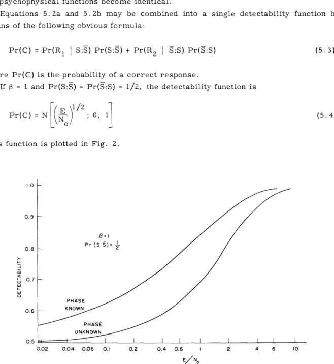
Equations 5. 2a and 5. Z2b may be combined into a single detectability function by means of the following obvious formula:
Pr(C) = Pr(R1 S:S) Pr(S:S) + Pr(R2 I S:S) Pr(S:S)
where Pr(C) is the probability of a correct response.
If = 1 and Pr(S:S) = Pr(S:S) = 1/2, the detectability function is
Pr(C) = N
)
; 0, 1This function is plotted in Fig. 2.
1.0 0.9 0.8 - I-0 U 0 0.7 0.6 0.5 (5. 3) (5. 4) Pr (S S)= 2 PHASE 0.02 0.04 0.06 0.1 0.2 0.4 0.6 1 2 4 6 10 E/No
Fig. 2. Ideal-detector psychophysical functions for the two-category forced-choice situation. Signal known exactly and known except for phase;
p = 1; Pr(S:S) = 1/2.
Case of the Signal Known Except for Phase. This case is solved in Appendix E for 3 = 1 only. From Eqs. E. 29 and E. 27 we have
Pr(R1 S:S) = - exp
L-2N
J (5. 5a)Pr(R1 | S:S) = exp -2N o (5. 5b)
Combining these two equations into a single detectability function by formula 5. 3 we have, for Pr(S:S) = Pr(S:S) = 1/2 (and = 1),1
Pr(C) = 1 - exp - 2 (5.6)
This equation is plotted in Fig. 2.
We have already discussed the advantages of the detection-theory model as it applies to the yes-no situation (section 3). Our comments apply equally well to the present forced-choice situation.
PART II. EXPERIMENTAL RESULTS AND DISCUSSION
6. INTRODUCTION
The experiments discussed in this report were undertaken with the aim of exploring the manner in which and the extent to which a human subject differs from an ideal detec-tor in the performance of an audidetec-tory detection task.
The two-category symmetrical forced-choice technique was used throughout. For a discussion of this technique and its advantages the reader is referred to Part I, sec-tion 4.
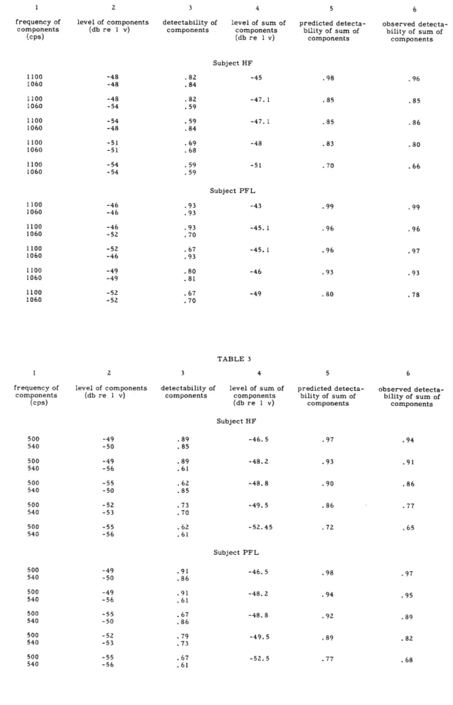
Two experiments were performed in order to measure with a considerable degree of accuracy the subjects' ability to detect auditory signals in the presence of broadband gaussian noise. Experiment 1 dealt with sinusoidal signals. Experiment 2 dealt with
signals having two sinusoidal components. All listening was monnaur.
25