S-1
Electronic Supporting Information
Removal of Cells from Body Fluids by Magnetic
Separation in Batch and Continuous Mode: Influence of
Bead Size, Concentration and Contact Time
Nils Bohmer1†, Nino Demarmels1†, Elena Tsolaki2, Lukas Gerken1, Kerda Keevend1, Sergio Bertazzo2,
Marco Lattuada3, Inge K. Herrmann1*
1Department Materials Meet Life, Swiss Federal Laboratories for Materials Science and Technology (Empa), Lerchenfeldstrasse 5, CH-9014, St. Gallen, Switzerland.
2Department of Medical Physics and Biomedical Engineering, University College London (UCL), Malet Place Engineering Building, London, WC1E 6BT, United Kingdom
3
Department of Chemistry, University of Fribourg, Chemin du Musée 9, CH-1700 Fribourg, Switzerland.
† contributed equally as first authors *[email protected]
S-2
Figure S1: Particle size and polydispersity index (PDI). Hydrodynamic size of magnetic beads in water
S-3
Mathematical Model
Closed form solution of Equations (1-5)
In order to find the closed form solution of the equations, we can proceed as follows. The equations are first rendered dimensionless. The following dimensionless quantities are defined:
0 0 0 2 1 1 3 b C MP C MP i i k T R R N t R R N N C y N (1.1)The equations can be written in dimensionless form:
1 0 0 0 1 1 1 1 1 1 1 M i i i i i M M d i y d M dy y d dy i i y y d M M dy y d M
(1.2)The initial conditions are:
0 0 0 0 0 for 1 0 1 T i C y r N y i M (1.3)Using the conservation of particles and cells, we can rewrite the first equation as follows:
1 1 d r d M (1.4)This equation can be solved exactly, and the solution reads:
1 1 exp 1 1 exp r r M M r r M M (1.5)
S-4 0 0 0 1 1 exp 1 1 exp 1 1 exp 1 M r r M M dy y d r r M M r r M M y r r M (1.6)
To integrate the other equations, we start taking the ratio of all cell balance equations with the one for y0. In this manner, the concentration of particles disappears. We have:
1 1 0 0 1 0 0 0 1 0 1 1 1 1 1 1 1 i i i M M dy y dy M y dy i y i y dy M y M y dy y d M y (1.7)
The solution can be written in the following general form:
1 1 1 1 0 0 0 0 1 i i i M M M M i M M r y y r y y i i y (1.8)
One can easily verify that this solution satisfies the mass balance on all cells:
1 1 0 0 0 0 i M i M M M M M i i i M y y r y r i
(1.9)The average number of particles per cell can be obtained as follows:
1 1 1 1 1 0 0 0 0 1 1 1 1 1 1 0 0 0 0 0 1 0 0 0 1 1 i M i M M M M M M i i i i M i M M M M M M M M i i i M i M i M i i M d i y y r y r i dr M M i y i y r y M r r y i i y y i M r y
(1.10)S-5
Finally, the final form of the solution is obtained by substituting Equation (1.6) into Equation (1.8) 1 1 1 1 exp exp 1 1 1 M i i r r r r M M M M M y r i r r M M (1.11) Solution of Equations (7-9)
For the solution of Equations (7-9), we proceed in a similar manner. The following dimensionless quantities are defined:
1, 0 1, 1, 2, 0 0 0 2, 2, 1, 1, 2 1 1 3 , , 1 1 1 1 b C MP C MP i i i i C MP C MP C MP C MP k T R R N t R R C C N y z N N N R R R R W R R R R (1.12)The equations can be written in dimensionless form:
1 2 1 2 1 1 0 1 0 2 0 0 1 1 1 1 1 0 0 1 2 2 1 1 1 1 1 1 1 1 1 M M i i i i i i i M M i i i M d i i y z d M M dy y d dy i i y y d M M dy y d M dz z d dz i i z z d M M dz d
1 2 M z M (1.13)S-6
The initial conditions are:
0 1 1 0 2 2 0 0 0 for 1 0 0 0 for 1 0 1 i i y r y i M z r z i M (1.14)The magnetic particles concentration conditions can be written as:
1 2 1 1 1 M M i i i i i y i z
(1.15)The solution of the cell populations equations in terms of y0 and z0, respectively, is:
1 1 1 2 2 2 1 1 1 1 0 1 0 1 1 1 2 0 2 0 i i M M M i i i M M M i M y y r y i M z z r z i (1.16)
The balance equation of particles can be reformulated as:
1 1 1 2 2 2 1 1 1 1 1 1 1 1 1 2 1 1 0 2 2 0 M M M M M M d r r r r y r r z d (1.17)
A relationship between y0 and z0 can be easily obtained:
0 0 0 0 0 0 2 1 dz z z y dy y r r (1.18)
Then, the equation for the particle concentration will be integrated as a function of y0:
1 2 2 1 1 2 2 1 2 1 1 1 1 1 1 1 1 0 1 2 1 2 1 0 2 2 0 0 0 0 0 1 1 0 0 1 1 2 2 1 1 1 1 1 M M M M M M M M M y r r r r d r y r r dy y y y y r y y v M r M r r r (1.19)
The only equation to be solved (numerically) is the following one, providing the concentration of cells without bound particles, as a function of time:
S-7 1 2 0 0 1 0 0 0 0 1 1 2 2 1 1 1 1 1 M M dy y d dy y y y M r M r d r r (1.20)
S-8
Figure S2: Mathematical modelling results for magnetic beads with a size of 300 nm. Unspecific
binding was included through the parameter . Two different ratios of specific versus unspecific cells were investigated: 0.2 and 10-5. Total contact time: 10 minutes. Change in the fraction of cells with at least 10 magnetic particles as a function of for both specific and unspecific cells. Four particles number concentrations: (a) 5 x 10⁹ beads per mL. (b) 5 x 10⁸ beads per mL. (c) 5 x 10⁷ beads per mL. (d) 5 x 10⁶ beads per mL.
a
b
S-9
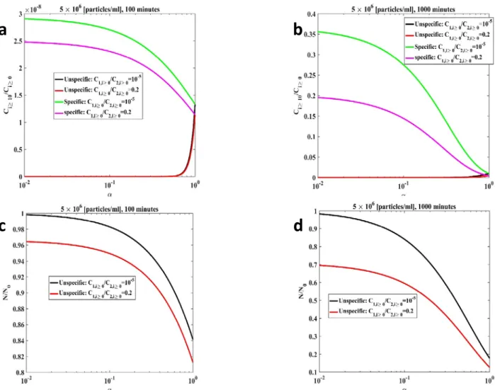
Figure S3: Mathematical modelling results for magnetic beads with a size of 300 nm. Unspecific
binding was included through the parameter . Two different ratios of specific versus unspecific cells were investigated: 0.2 and 10-5. Particles number concentration 5 x 10⁶ beads per mL. (a) Change in the fraction of cells with at least 10 magnetic particles as a function of for both specific and unspecific cells, contact time 100 minutes. (b) Change in the fraction of cells with at least 10 magnetic particles as a function of for both specific and unspecific cells, contact time 1000 minutes. (c) Change in the concentration of magnetic particles as a function of for both specific and unspecific cells, contact time 100 minutes. (d) Change in the concentration of magnetic particles as a function of for both specific and unspecific cells, contact time 1000 minutes.