Higher SLA Satisfaction in Datacenters with Continuous Placement Constraints

HAL Id: hal-00932201

https://hal.inria.fr/hal-00932201

Submitted on 23 Oct 2014

HAL is a multi-disciplinary open access archive for the deposit and dissemination of sci-entific research documents, whether they are pub-lished or not. The documents may come from

L’archive ouverte pluridisciplinaire HAL, est destinée au dépôt et à la diffusion de documents scientifiques de niveau recherche, publiés ou non, émanant des établissements d’enseignement et de

Higher SLA Satisfaction in Datacenters with Continuous

Placement Constraints

Tu Dang

To cite this version:

Tu Dang. Higher SLA Satisfaction in Datacenters with Continuous Placement Constraints. Operating Systems [cs.OS]. 2013. �hal-00932201�

Polytech Nice-Sophia University

Master IFI - Ubinet Track

Higher SLA Satisfaction in

Datacenters with Continuous

Placement Constraints

Author:

Huynh Tu Dang

Supervisor:

Prof. Fabien Hermenier

Tutor:

Prof. Giovanni Neglia

Higher SLA Satisfaction in Datacenters with

Continuous Placement Constraints

By

Huynh Tu Dang

Polytech Nice-Sophia, 2013

Acknowledgments

I would like to express my gratitude to my supervisor Professor Fabien Hermenier for his useful comments, remarks and engagement through the learning process of this thesis. This research project would not have been done without his support. I would also like to thank Professor Giovanni Neglia for reading my final project report and my thesis. Furthermore, I would like to thank Professor Fabrice Huet for reading my research paper and his technical support. Also, I I would like to thank Professor Guillaume Urvoy-Keller and Professor Lucile Sassatelli for their ultimate support on the way. In addition, I like to thank other people as OASIS team who have willingly shared their precious time during the process of the thesis.

Higher SLA Satisfaction in Datacenters with Continuous

Placement Constraints

Huynh Tu Dang

Polytech Nice-Sophia University Sophia, Antipolis

2013

ABSTRACT

In a virtualized datacenter, the Service Level Agreement for an application restricts the Virtual Machines (VMs) placement. An algorithm is in charge of maintaining a placement compatible with the stated constraints.

Conventionally, when a placement algorithm computes a schedule of actions to re-arrange the VMs, the constraints ignore the intermediate states of the datacenter to only restrict the resulting placement. This situation may lead to temporary constraint violations. In this thesis, we present the causes of these violations. We then advocate for continuous placement constraints to restrict also the action schedule. We discuss why the development of continuous constraints requires more attention but how the extensible placement algorithm BtrPlace can address this issue.

Table of Contents

1 Introduction . . . 1 1.1 Problem Statement . . . 1 1.2 Contributions . . . 2 1.3 Outline . . . 3 2 Literature Review . . . 4 2.1 Cloud Computing . . . 4 2.1.1 Deployment models . . . 5 2.1.2 Characteristics . . . 5 2.2 Virtualization . . . 6 2.3 Virtualized Datacenter . . . 8

2.3.1 SLA to VM Placement Constraint . . . 9

2.3.2 VM Placement Algorithm . . . 9

2.3.3 Current Btrplace . . . 12

3 Reliability of Discrete Constraints . . . 15

3.1 Discrete constraints . . . 15

3.2 Evaluation Results . . . 18

3.2.1 Simulation Setup . . . 18

3.2.2 Evaluating Temporary Violations . . . 20

4 Elimination of Temporary Violations with Continuous Constraints 23 4.1 Continuous constraint . . . 23

4.2 Modeling the continuous constraints . . . 24

4.2.1 MaxOnlines . . . 24

4.2.3 MinSpareResource(S, r, K) . . . 27

4.3 Trade-off between reliability and computability . . . 29

4.3.1 Reliability of continuous constraints . . . 29

4.3.2 Computational overheads for continuous constraints . . . 30

5 Conclusion . . . 31

List of Figures

1.1 discrete satisfaction . . . 2

1.2 continuous satisfaction . . . 2

2.1 An usual server and a virtualized server [1] . . . 6

2.2 A virtualized datacenter with there server racks[2] . . . 8

2.3 dynamic VM placement Algorithm . . . 11

2.4 c-slice and d-slice of a VM migrating from N1 to N2 . . . 14

3.1 Examples of spread, among, SplitAmong and maxOnlines constraints . . 16

3.2 Distribution of the violated constraints . . . 21

4.1 Modeling Power-Start and Power-End of a node . . . 25

4.2 Cumulative scheduling of maxOnlines constraint . . . 25

4.3 Modeling idle period of a node . . . 26

4.4 Solved instances depending on the restriction. . . 29

List of Tables

2.1 Variables exposed by Reconfiguration Problem . . . 13

3.1 VM characteristics . . . 19

Chapter 1

Introduction

Cloud computing offers attractive opportunities to reduce costs, accelerate develop-ment, and increase the flexibility of the IT infrastructures, applications, and services. Virtualization techniques, such as XEN [3], VMware [16], and Microsoft Hyper-V [18], that enable the applications to run in a virtualized datacenter by embedding the appli-cations in virtual Machines (VMs). The appliappli-cations often require Quality of Service (QoS) while they are hosted on the cloud. The QoS are expressed in a Service Level Agreement (SLA) which is a contract between the customer and the service provider specifying which services the service provider will furnish. Application components can run on distinct VMs and the VMs composing an application are arranged in the dat-acenter to meet the QoS of the application. A VM placement algorithm is needed to assign for each VM a placement, and compute a reconfiguration plan to transform the datacenter to the viable state which satisfies the SLAs simultaneously. Current place-ment algorithms [4, 5, 6, 7, 8, 9] rely on the discrete placement constraints which only restrict the VM placements on the result configuration. It is possible for a reconfig-uration to temporarily violate a SLA, such as the temporary co-locating of the VMs required to be separated or vice versa.

1.1

Problem Statement

Datacenters may have to reconfigure due to the variation of workloads, hardware main-tenance, or energy objective. A placement constraint which only restricts the final assignment of VMs may lead to a temporary violation of a SLA during the reconfig-uration. For example, Figure 1.1 illustrates the temporary violation of the SLA that requires the placement separation of VM1 and VM2. Initially, VM1 runs on N1 and VM2 is waiting for being deployed. VM2 can run only on N1 due to its resource require-ment. The placement of VM1 and VM2 are separated at the beginning and at the end of the reconfiguration. However, between time t0 and t1, these VMs are co-located on

the same node. Figure1.2 shows this temporary violation can be prevented by delaying the start of VM2 until the end of VM1’s migration.

In this work, we attempt to solve the temporary violation problem of placement con-straints during datacenter reconfiguration. This problem can be divided into several sub-problems, as follows:

Fig. 1.1: discrete satisfaction Fig. 1.2: continuous satisfaction

• How datacenter reconfiguration relying on discrete constraints violates application SLAs and which SLAs are likely violated?

• How continuous constraints can help a placement algorithm eliminate these tem-porary violations?

• How continuous constraints affect on a placement algorithm to schedule actions leading to the viable configuration?

1.2

Contributions

Using BtrPlace, a VM placement algorithm for cloud platforms, we found a solution for the problems above. The contributions of this thesis can be summarized as follows:

• We study the static and dynamic VM placement algorithms.

• We demonstrate temporary violations of SLAs during reconfiguration by means of BtrPlace, a dynamic placement algorithms replying on discrete constraints. • We propose continuous constraints to support the VM placement algorithm in

preventing the temporary violations.

• We model and implement the discrete and continuous constraints, including

Max-Online, MinSpareNode, MaxSpareNode and MinSpareResource using BtrPlace.

• We evaluate the effects of continuous constraints on the computation of Reconfig-uration Problem.

Realizing the limited study for continuous SLAs satisfaction in datacenters, we have published our finding in the 9th Workshop on Hot Topics in Dependable Systems.

1.3

Outline

The rest of the thesis is organized in several chapters as follows: Chapter2provides the background of cloud computing, as well as discusses the static and dynamic placement algorithms to reconfigure datacenters. Chapter 3 presents the definition and model of discrete placement constraints and exhibits their temporary violations during datacenter reconfiguration. Chapter4 introduces the model of continuous constraints and reports some preliminary results of continuous constraint implementation in order to eliminate the temporary violations. Chapter5concludes this thesis and proposes future research.

Chapter 2

Literature Review

This chapter presents the background of the thesis and the related work materials con-cerning virtual machine placement. The same concon-cerning virtual machine placement constraints for continuous satisfaction of application requirements are also studied. Our work is positioned in the next level of the placement constraint as it leverages dynamic placement algorithms to include not merely the placement problem but a more reliable reconfiguration action schedule.

2.1

Cloud Computing

Cloud Computing [10] is the computing paradigm which enables remote and on-demand access to configurable computing resources offering them as services while min-imizing the human efforts to configure these resources. Depending on the kind of services three different forms of cloud services [11] can be found:

• Software as a Service (SaaS) consists of any online application that is normally run in a local computer. SaaS is a multi-tenant platform that uses common resources and an instance of application as well as the underlying database to support mul-tiple customers as the same time. An end user can access data and applications on the cloud from everywhere. Email hosting and social networking are common applications in which a user can access his data through a website providing his username and password. For example, web mail clients, Google Apps are among the cloud-based applications.

• Platform as a Service (PaaS) provides developers the access to a software plat-form where applications are built upon, like Google App Engine and Window Azure. Comparing to traditional software development, this platform can reduce the development time, offer readily available tools and quickly scale as needed. • Infrastructure as a Service (IaaS) enables access to computing resources, such as

network, storage and processing capacity. This model is flexible for customers since they pay as they grow. There is no need for the customers to plan ahead for their demands of infrastructure. Enterprises use the cloud resources to supplement the resources they need. Cloud storage can be used for backup data and cloud

computing power can be used to handle the additional workloads. Amazon EC2, RackSpace, . . . are typical examples for this cloud form.

2.1.1

Deployment models

There are four primary deployment models recommended by the National Institute of Standards and Technology (NIST):

Public Cloud provides services and infrastructure to various clients on the basis of a

pay-per-use license policy. This model is best suitable for the start-up business or the business requiring load spikes management. This model helps to reduce the capital expenditure and operational IT costs.

Private Cloud refers to the internal datacenter of an organization when it is large enough

to benefit from the advantages of cloud computing. When moving to the cloud, orga-nizations have to deal with the data security related to the cloud, such as data privacy, and operation audits. This model takes care of these concerns.

Hybrid Cloud takes advantages of both Public Cloud and Private Cloud as it secures

confidential applications and data by hosting them on the private cloud while sharing public data on the public cloud. This model also helps to handle the bursting workloads in the private cloud by acquiring additional computing power in the public cloud to absorb the bursting workloads.

Community Cloud is the cloud infrastructure collaborated by several organizations

which have the same interests to reduce the costs as compared to own a private cloud. This model is designed to support research into the design, provisioning, and manage-ment of services at a global, multi-datacenter scale.

2.1.2

Characteristics

To provide the cloud platform, a cloud provider should have the following characteristics of cloud computing:

• Rapid Elasticity: The ability to scale the resources up and down as needed. Customers can purchase as much or as little computing power depending on their needs.

• Measured Service: Services are controlled and monitored by cloud providers. It is important for the customers to assert whether the performance of their services is satisfied by the cloud providers.

• On-Demand Self-Service: Customer services run as needed without any human interaction.

• Ubiquitous Network Access: Services can be accessed through standard mech-anisms by both thick and thin clients.

• Resource Pooling Physical and virtual resources are served via multi-tenant model. Depending on customer demand, resources are allocated and reallocated as needed. The customers can also specify the location of resources hosting their service through high level abstraction constraints.

Scope of the thesis In this thesis, we focus on IaaS clouds that primarily rely on virtualization technologies. We develop the high level abstraction of requirements for resource location in public clouds. These requirements provide better Quality of Ser-vices for the cloud-based applications by eliminating the temporary violations that are explained in the next chapter. As a result, the cloud providers can offer better services for critical applications and cloud infrastructure.

2.2

Virtualization

Virtualization [12] is the abstraction of hardware platform, operating system, storage, or network devices to share the resources among users. The most important part of virtualization is virtual machine, an isolated software container with an operating system and applications inside. A thin virtualization layer called hypervisor decouples the VMs from the physical node (node is equivalent to server). Each VM appears to have its own processor, memory and other resources (Figure 2.1). The hypervisor controls the processors and resources of a physical node and dynamically allocates them to each VM as needed. The hypervisor guarantees that each VM cannot disrupt each other.

Fig. 2.1: An usual server and a virtualized server [1]

A hypervisor enables many VMs to run concurrently on a single physical node, providing better hardware utilization and isolation as well as application security and mobility. Every physical node is used to its full capacity. This feature significantly reduces the operational costs by deploying fewer nodes overall. A running VM can be transferred

from one physical node to another using a process called live migration. Critical appli-cations can be also virtualized [13] to improve performance, reliability, scalability and reduce deployment costs.

Virtualization increases the resource utilization. Most computers do not fully utilize their resources which leads to inefficient energy usage [14]. A solution is installing more applications on one computer but this way may cause conflicts between the applica-tions. Another possible problem is a single Operating System failure will take down all the applications running in that system [15]. Virtualization is the solution that allows the applications to run on the same node but isolates them to avoid the con-flicts. Furthermore, virtualization also provides other advantages such as scalability, high availability, fault tolerance, and security which are hardly achieved by traditional hosting environment.

There are two types of virtualization: bare-metal and hosted. A Bare-metal hypervisor means the hypervisor is installed directly onto the server hardware without the need for a pre-installed OS on the server. XEN [3], VMware ESXi [16], Citrix XenServer [17] and Microsoft Hyper-V [18] are examples of bare-metal hypervisors. On the other hand, a Hosted hypervisor means the hypervisor is installed as a usual application in the Op-erating System installed on a server. Hosted hypervisors include VMware Workstation, Fusion, VMware Player, VMware Server. Microsoft Virtual PC, Microsoft Server, and Sun’s VirtualBox [19]. Bare-metal hypervisors installed right on the server hardware and therefore offer higher performance and support more VMs per physical CPU than

hosted hypervisors [20].

Live migration [21] is a technique to move a running VM from one physical node to another with minimal service downtimes. Live migration is performed by taking a snapshot of the VM and coping its memory states from one physical node to another. Then the VM on the original node is stopped after the copy version has run successfully on the new node.

There are many ways for moving the content of the VM memory from one node to another. However, migrating a VM requires the balance of minimizing both downtime and total migration time. The former is the unavailable duration of the service because there is no currently executing instance of the VM. The latter is the duration between the start moment of migration and the moment of the origin VM being discarded. To ensure the consistency of the VM during the migration, the migration process is viewed as a transaction between two involved nodes. A target node which satisfies the resources requirement is selected. A VM is requested on the target node and if this fails, the origin VM continues running unaffectedly. All data are transferred from the origin node to the target node. Then the origin VM is suspended and its CPU state is transferred to the target node. After the target VM is in consistent state, the origin VM can be discarded on the origin node to release the resources.

Migrating VMs [21] across distinct physical nodes is a useful tool for datacenter admin-istration. It facilitates fault management, load balancing, and system maintenance in

datacenters without or minor disrupting application performance.

2.3

Virtualized Datacenter

A virtualized Datacenter is a pool of cloud infrastructure resources designed specifically for enterprise business needs. Those resources include compute, memory, storage and bandwidth. They are made available for cloud customers to deploy and run arbitrary software which can include Operating Systems and applications.

A virtualized datacenter consists of hosting nodes (servers) providing the resources and applications embedded in VMs consuming the resources. Nodes in a rack connect to the top-of-rack switch which connects to the upper level switches or routers. Figure2.2

depicts a small virtualized datacenter which consists of three racks. VMs are delivered to employees through the central VM manager. The virtualized datacenter is divided into there zones and each zone can host only the VMs that delivered to the employees belonging to that zone. For instance, the VM of a finance staff can only be hosted in Finance Zone for security concerns.

Fig. 2.2: A virtualized datacenter with there server racks[2]

Customers pay for using computing resources of cloud providers and usually they re-quire specific QoS to be maintained by the providers in order to meet their objectives

and sustain their operations. The performance metric and other restrictions related to security and availability of an application are formulated in a service level agreement.

2.3.1

SLA to VM Placement Constraint

A service-level agreement (SLA) is a contract between a service provider and a customer that specifies which services the provider will furnish and the penalties in case of violat-ing the customer expectations. Many service providers provide their customers a SLA so that services of their customers can be measured, justified, and perhaps compared with those of outsourcing providers. Cloud providers need to consider and meet different QoS parameters of each individual customer as negotiated in the specific SLA. Usually, a SLA is expressed in a VM placement constraint.

A VM placement constraint [22] restricts the placement of a VM or a set of VMs. The typical VM placement constraint ensures sum of the demands in terms of CPU, memory and slots of the VMs placed on a certain node does not exceed the node’s capacities in these resources.

Other VM placement constraints include location and collocation rules [23]. The loca-tion and anti-localoca-tion constraints restrict or disallow a VM to place on a certain node, respectively. The collocation and anti-collocation constraints are used to place some VMs on the same node, or to place them on distinct nodes. Other advanced constraints can maximize the load balancing between nodes [24,25] or minimize the energy cost for hosting VMs in datacenters [4, 26].

Traditional resource management is no longer provide incentives for cloud providers to share their resources with regards to all service requests. A QoS-based resource allocation mechanism is necessary to regulate the supply and demand of cloud resources for both cloud customers and providers. In virtualized datacenters, VM placement algorithms are used to regulate the resource allocation.

2.3.2

VM Placement Algorithm

A placement algorithm is the datacenter’s intelligence used to allocate the resources to the applications in the way that satisfies application requirements simultaneously. The placement algorithms are used to improved the scalability [27,28], performance [29,30], and reliability [31,7] of the applications by automatic computing and migrating the VMs due to network affinity, workload variation, and system maintenance. The placement algorithms find the placement for each VM to satisfy simultaneously the application requirements and the datacenter objective such as load balancing or energy saving. The common technique is finding a configuration that maps the VMs on the minimum of nodes and migrating the VMs across the network to reach the found configuration.

The problem of placing N VMs on M nodes is often modeled as a vector-packing problem, assuming that the resource demands remain stable during the re-arrangement of VMs [25]. The physical nodes are modeled as one or more dimensions bins and the VMs are the items with the same number of dimensions to be put into these bins. In order to find the optimized mapping, a complete search by enumerating all the possible combinations is needed and the complexity becomes NP-hard. To solve this problem, heuristic solutions have been proposed such as algorithms derived from vector-packing algorithms [32,31,26]. There are two types of VM placement algorithm including static and dynamic VM placement algorithm.

Static VM Placement Algorithm

A static VM placement algorithm is used to optimize the initial resource allocation for workloads through a configuration to improve application performance, reduce the costs of infrastructure and increase the scalability of datacenters [33, 27, 34]. The configura-tion is not recomputed for a long time until the datacenter administrator re-runs the algorithm. This strategy leaves many physical servers running at a low utilization for most of the time [14].

Meng et al. [27] design the two-tier approximate algorithm that deploy VMs in large scale datacenters. Chaisiri et al. [33] consider the deployment cost of applications on multi-datacenters environment. Xu et al. [34] expand the two-level control management in which local controllers determine the application resource demands and a global con-troller determines the VM placement and resource allocation to minimize the power consumption while maintaining the application performance. These algorithms is miss-ing the ability of recomputmiss-ing the VM placement at runtime when applications vary their loads or in the event of network and server failures.

Dynamic VM Placement Algorithm

Because of the limitation of static placement algorithms, dynamic placement algorithms are used to deploy the new VMs in a datacenter and computes a new mapping in the event of variation of workloads, datacenter maintenance or efficient energy consolida-tion. Dynamic placement algorithms recompute the datacenter configuration in shorter timescales, preferably shorter than the major variation of application workloads. The historical resource utilization and application requirements are used as the input to the algorithms that deploy VMs in datacenters. Dynamic placement algorithms leverage the live migration ability.

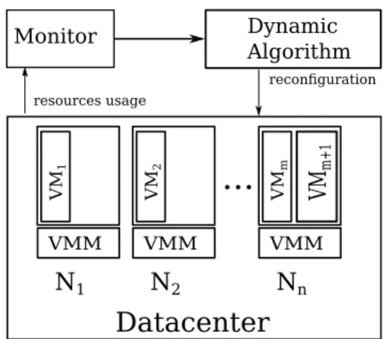
A dynamic placement algorithm computes a new configuration when there is a change in datacenter environment, such as workload variations, hardware failures. Figure 2.3

presents the architecture of a dynamic placement algorithm. The monitor component monitors the resource usage in the datacenter. The monitor component then combines

Datacenter

VMM VM 1 N₁ VMM VM m N_n VMM VM 2 N₂ VM m+ 1

...

Monitor resources usage Dynamic Algorithm reconfiguration

Fig. 2.3: dynamic VM placement Algorithm

the resource usage with the application and datacenter constraints to input into the

dynamic placement algorithm component. The dynamic placement algorithm computes

a reconfiguration plan to transfer the datacenter from current configuration to the new configuration. Actions in the reconfiguration plan are scheduled for execution to satisfy VM placement constraints such as maximum capacity or anti-collocation constraint. Entropy [4] and Wood et al. [35] consider the action schedule in their placement algo-rithms. They justify the need to solve dependencies between migrations. Their adhoc heuristics to treat the action scheduling disallow however the addition of any placement constraints. Bin et al. [36] provide the k-resilient property for a VM in case of server failures. The algorithm provides a continuous high-availability by scheduling to migrate only the VMs marked as highly-available. This approach disallows temporary violations but limits the management capabilities of the VMs to this particular use case.

Authors in [29, 7, 5] propose algorithms that support an extensible set of placement constraints. They however rely on a discrete approach to compute the placement. In [7, 5], a node is chosen for every VM randomly. The choice must satisfy the constraints once the reconfiguration completed but it is still possible to make two VMs involved in an anti-collocation constraint overlap (see Figure 1.1). Breigand et al. [29] use a score function to choose the best node for each VM. The same temporary overlap may then appear if putting the first VM on the node hosting the second one leads to a better score.

Entropy [4] and BtrPlace [7] (successor to Entropy) are resource managers based on Constraint Programming. They performs dynamic consolidation to put VMs on a re-duced set of nodes. Entropy and BtrPlace use Choco [37], an open-source constraint solver, to solve a Constraint Satisfaction Problem where the goal is minimizing the num-ber of the running nodes and minimizing migration costs. Furthermore, BtrPlace can be dynamically configured with placement constraints to provide the Quality of Service for applications in a datacenter.

2.3.3

Current Btrplace

BtrPlace is a configurable and extensible consolidation manager based on constraint programming. BtrPlace provides a high-level scripting language to describe application and datacenter requirements. It provides an API to develop and integrate new place-ment constraints. BtrPlace is scalable since it exploits possible partitions implied by placement constraints, which allows solving sub-problems independently.

Constraint Programming

Constraint Programming (CP) [38] is used to model and solve combinatorial problems by stating the constraints on the feasible solutions for a set of variables. The solving algorithm of CP is independent of the constraints composing the problem and the order in which they are provided. A problem is modeled as a Constraint Satisfaction Problem (CSP) which consists of a set of variables, a set of domains, and a set of constraints. A domain is the possible values of a variable and a constraint represents the required relations between the values of the variables. A solution of a CSP is an assignment of a value to each of the variables that satisfies all the constraints simultaneously. The primary benefit of CP is the ability to find the global optimum solution. However, in the dynamic VM placement problem, it is more important to provide an optimized solution in a limited time frame.

BtrPlace allows the data center and application administrator to define their con-straints independently. In this section, we briefly introduce the BtrPlace architecture. Then we describe how BtrPlace models a Reconfiguration Problem.

Architecture

BtrPlace abstracts a datacenter infrastructure in a Model including nodes, VMs, re-source capacity of nodes, rere-source demand of VMs, state of nodes and VMs. The expectation of datacenter and application administrators are expressed in placement

constraints. The model and constraints are inputted in the reconfiguration problem

which produces a reconfiguration plan to transform the datacenter to the new viable configuration.

Reconfiguration Problem

A Reconfiguration Problem (RP) is the problem of finding a viable configuration that satisfies all the placement constraints and a reconfiguration plan to transform current configuration into the computed one. A reconfiguration plan consists of a series of action that related to VMs and node management such as migrating VM, turning-off

or booting VM or node. The actions are scheduled based on their duration to ensure their feasibility. For instance, a migration action is feasible if the target node in the destination configuration has sufficient amount of CPU and memory during and after the reconfiguration. Besides satisfying all placement constraints, a reconfiguration plan may have to satisfy with the time constraints.

Variable related to Mapping vh

i current host of VM i

v_iq state of VM i nqj state of node j

nvm

j the number of VMs hosted by node j

Variable related to ShareableResource vr

i amount of resources allocated to VM i

nr

j resource capacity of node j

Variable related to action Management as

i, aei moments action i starts and ends, respectively

ad

i execution duration of action i

Table 2.1: Variables exposed by Reconfiguration Problem

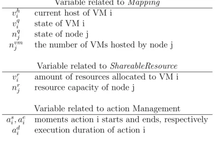
Modeling a Reconfiguration Problem Using CP, a reconfiguration problem is defined in BtrPlace includes: a model and a set of constraints. The set of nodes N and the set of virtual machines V are included in the reconfiguration problem. The set of variables exposed by a RP is summarized in Table 2.1. Developers use these variable sets to implement new placement constraints.

A model consists of Element, Attributes, Mapping and View. An element is a VM or a physical node which has several optional attributes. A Mapping indicates the state of VMs and nodes as well as the placement of the VMs on the nodes. In a Mapping, a node nj is represented by its state nqj that is either 1 if the node is online or 0 otherwise.

The variable vh

i = j indicates the VM vi is running on the node nj. For each dimension

of resources, a View instance provides a domain-specific information of a model. For example, The ShareableResource is a View that defined the resource capacity of nodes and resource demand of VMs. A node nj provides an amount of resources of nrj. A VM

vi is considered to consume a fixed amount of resources vri. In addition, the variables

related to action management including as_{, a}e _{denoting the start and the end moment}

of an action respectively. ad _{denotes the duration of the action.}

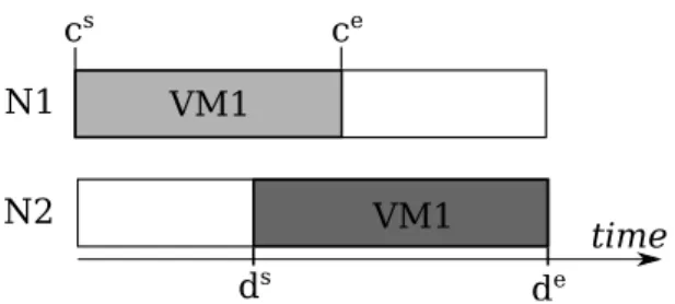
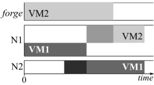
Beside the variables exposed in RP, developers can introduce additional variables as needed. To support for the reconfiguration algorithm, a slice notation is introduced in BtrPlace (Figure 2.4). A slice is a finite period indicates a VM is running on a node and consuming the node’s resource. The height of a slice equals the amount of

N1 N2 VM1 VM1 ce ds de cs time

Fig. 2.4: c-slice and d-slice of a VM migrating from N1 to N2

consumed resources. There are consuming slice and demanding slice for a VM involved in a reconfiguration problem. A consuming slice (c-slice) ci ∈ C of a VM vi is the period

which starts at the beginning of the reconfiguration process and terminates at the end of the VM migration action. Similarly, a demanding slice (d-slice) starts at the beginning of the VM migration action and terminates at the end of reconfiguration process. BtrPlace provides the set of placement constraints related to resource management, isolation, fault tolerance, and server management. The set of constraints include the (anti-)affinity rules in VMware DRS [23] and the VM placement features available in Amazon EC2 [39]: availability-zones and dedicated instances. However, the current implementation of the constraints focuses on discrete approach which restricts only the final placement of the VMs. It can cause the temporary violations of the constraints. In this thesis, using BtrPlace library I demonstrate the temporary violations of the placement constraints during reconfiguration of datacenters and provide a solution to prevent these violations.

Chapter 3

Reliability of Discrete Constraints

Many computing service providers are deploying datacenters to deliver Cloud computing services to customers with particular Quality of Services requirements. These require-ments are often translated into placement constraints for dynamic provisioning. Most of dynamic placement algorithms rely on the discrete constraints [4,35,29,7,5]. However, this approach may cause the temporary violations of the QoS during the reconfigura-tion. This chapter presents the discrete placement constraints and the evaluation of their reliability during the datacenter reconfiguration. The first part presents the defi-nition, practical interest and model of the discrete placement constraints. The second demonstrates the evaluation method, and the temporary violations of discrete placement constraints. We rely on BtrPlace to provide the implementation of discrete constraints and to exhibit the temporary violations that are allowed by the use of discrete con-straints.

3.1

Discrete constraints

A discrete constraint is a VM placement constraint that imposes the satisfaction of the constraint only on the destination configuration. The discrete constraint ensures the viability of the destination configuration when the constraint is not satisfied in the current configuration.

BtrPlace provides many placement constraints covering in isolation, high availability, and high performance. We select some constraints that commonly exists in practice to evaluate their reliability during the reconfiguration, including spread (anti-affinity VM-VM DRS [23]), among (VM-Host affinity DRS), splitAmong (Availability Zones EC2 [39]), SingleResourceCapacity, and MaxOnlines. In the next subsection, we present the definition, practical interest of these constraints.

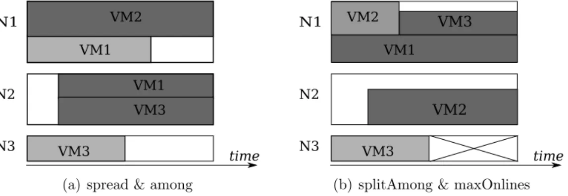
spread(M)

The spread constraint keeps the given VMs on distinct nodes in the destination recon-figuration. An example of a spread constraint spread(vm1,vm2) that separates VM1 and VM2 is shown in figure 3.1(a). In the destination configuration, this constraint is

satisfied as VM1 residing in N1 and VM2 residing in N2. An application administra-tor may use a spread constraint to provide the fault tolerance for his application. By spreading replicas, the application will be available as long as one replica is still alive.

dhi 6= d h

j ∀vi, vj ∈ M, i 6= j (3.1)

In equation (3.1), for the VMs in set M (M ⊂ V), the destination placement of each VM has to be different from each other.

N1 N2 VM1 VM1 time VM2 N3 _VM3 VM3

(a) spread & among

N1 N2 VM1 time VM2 N3 _VM3 VM3 VM2

(b) splitAmong & maxOnlines

Fig. 3.1: Examples of spread, among, SplitAmong and maxOnlines constraints

among(M, G)

The among constraint limits the placement of the given VMs on a set of nodes among the given sets G. In figure 3.1(a), the among constraint among({vm1,vm3},{{N1,N3},

N2}} keeps VM1 and VM3 on either set {N1,N3} or N2. Because VM1 and VM3

must be in the same set, VM1 is scheduled to move in N1, then VM3 is also migrated to N3. Datacenter and application administrators can use among constraints to group related VMs with regards to specific criteria. For example, the application having high communication between VMs may require to host its VMs on a set of nodes that connect to the same edge switch.

dhi ∈ X =⇒ d h

j ∈ X ∀i, j ∈ M, i 6= j, ∀X ∈ G (3.2)

In equation (3.2), if the host of VMi belongs to the set X, (X ∈ G), then all the VMs

in the set M are required to place in the hosts belonging to the set X. splitAmong(H, G)

The splitAmong constraint restricts several set of VMs on distinct partitions of nodes. In figure 3.1(b), the constraint splitAmong({{vm1,vm3},vm2}, {{N1,N3},N2}) is used

to separate the set {VM1, VM3} from VM2. VM1 and VM2 are co-located at the beginning, then one of them must be migrated to another node. VM2 is scheduled to migrate to N2. Furthermore, N3 must be shutdown for energy efficiency, VM3 cannot migrate to N2 because VM3 and VM2 have to be on different set. Then VM3 is scheduled for migrating to N1. In the end, different sets of VMs are on distinct partitions of nodes, then the constraint is satisfied. The splitAmong constraint can provide the disaster recovery property for applications. An application may have multiple replicas and each replica is hosted in a distinct zone of the datacenter. In case of disasters, the application still runs without any downtime period.

H is sets of VMs and G is a partitions of nodes. For all VMi and VMj in the same set

(∀i, j ∈ A), VMi and VMk in different sets (∀i ∈ A ∧ k ∈ B, A ∩ B = ∅), A, B ∈ H, we

have: dh i ∈ X =⇒ (d h j ∈ X ∧ d h k ∈ X),/ X ∈ G (3.3)

In equation (3.3), when a VMi is place on a node belonging to the set X, then the other

VMs are in the same set with VMi have to place on the nodes in the set X and the

VMs are not in the same set with VMi must not place on the nodes in the set X.

SingleResourceCapacity(S, r, K)

The SingleResourceCapacity constraint limits the number of resources for VM pro-vision of each node in a set of nodes. The practice interest of this constraint is to reserve resources for the hypervisor management run on each node to guarantee the performance of the hypervisor.

nrj − X d∈D dh i=j dri ≤ K ∀nj ∈ N , j ∈ S (3.4)

In equation (3.4), The resource r of each node in the set S is required to leave some idle resources and this amount is equals to the specified number K.

maxOnlines(S, K)

the maxOnlines constraint restricts the number of online nodes simultaneously. An example of maxOnlines constraint is applied in the configuration in the example3.1(b).

maxOnlines({N1,N2,N3},2) allows only 2 nodes to be online at the same time, then N3

is selected to go offline to satisfy the constraint. The practical interest of maxOnlines constraint is the license restriction or the limitation on capacity of power or cooling system. Datacenter administrator has to limit the number of online nodes in the data-center to satisfy the license or to prevent the overload of power or cooling systems. A

discrete maxOnlines constraint is modeled as the cardinality of online nodes has to be less than the number that specified in the constraint.

card(nq_j = 1) ≤ K, ∀nj ∈ N , j ∈ S (3.5)

In equation (3.5), the state of a node nqj equals to 1 means the node is online. Then the

cardinality of the online nodes in the set of nodes S must be less than or equals to the specified number K.

3.2

Evaluation Results

We evaluate here the reliability of discrete constraints presented in the previous section. We simulate a datacenter subject to common reconfiguration scenarios and inspect the computed reconfiguration plans to detect temporary violations.

3.2.1

Simulation Setup

We describe the datacenter setup, applications with Service Level Agreement (SLA) and the reconfiguration scenarios that existed in real datancenters.

Datacenter

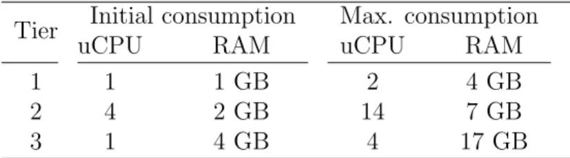
The simulated datacenter consists of 256 nodes split over 2 clusters. Each cluster consists of 8 racks of 16 nodes each. Inside a rack, nodes are connected through a non-blocking network. Each node has 128 GB RAM and a computational capacity of 64 uCPU, a unit similar to ECU in Amazon EC2 [39] to abstract the hardware. We simulate 350 3-tier web applications, each having a structure generated randomly to use between 6 and 18 VMs, with 2 to 6 VMs per tier. At total, the datacenter runs 5,200 VMs. Table 3.1

summarizes the VM resource consumption for each tier. VMs in the Tier 1 require a few and balanced amount of resources. VMs in the Tier 2 and 3 are computation and memory intensive, respectively. By default, each VM consumes only 25% of the maximum allowed. This makes the datacenter uCPU and memory usage equal to 68% and 40% respectively.

SLAs in the datacenter

A SLA is attached to each application. For each tier, one spread constraint requires distinct nodes for the VMs to provide fault tolerance. This mimics the VMWare DRS anti-affinity rule. One among constraint forces VMs of the third tier to be hosted on

Tier Initial consumption Max. consumption

uCPU RAM uCPU RAM

1 1 1 GB 2 4 GB

2 4 2 GB 14 7 GB

3 1 4 GB 4 17 GB

Table 3.1: VM characteristics

a single rack to benefit from the fast interconnect. Last, 25% of the applications use a splitAmong constraint to separate the replicas among the two clusters. This mimics Amazon EC2 high-availability through location over multiple availability zones.

The datacenter is also subject to placement constraints. The maximum number of online nodes is restricted to 240 by a maxOnlines constraint to simulate a hypervisor-based licensing model [17]. The 16 remaining nodes are offline and spread across the racks to prepare for application load spikes or hardware failures. Last, one singleResourceCa-pacity constraint preserves 4 uCPU and 8 GB RAM on each node for the hypervisor management operations.

Reconfiguration scenarios

On the simulated datacenter, we consider four reconfiguration scenarios that mimic industrial use cases[40]:

Vertical Elasticity. In this scenario, applications require more resources for their VMs to support an increasing workload. In practice, 10% of the applications require an amount of resources equals to the maximum allowed. With BtrPlace, this is expressed using preserve constraints to ask for resources.

Horizontal Elasticity. In this scenario, applications require more VMs to support an increasing workload. In practice, 25% of the applications double the size of their tiers. With BtrPlace, this is expressed using running constraints to ask to run more VMs.

Hardware Failure. Google reports that yearly, a network outage makes 5% of the servers instantly unreachable. [41] This scenario is simulated by setting randomly 5% of the nodes in a failure state and asking to restart their VMs on other nodes.

Boot Storm. In virtual desktop infrastructures, numerous desktop VMs are started simultaneously before the working hours. To simulate this scenario, 400 new VMs are required to boot. Their characteristics are chosen randomly among those described in Table 3.1 and their resource consumption is set to the maximum allowed.

3.2.2

Evaluating Temporary Violations

For each scenario, we generate 100 different instances that satisfy the placement con-straints. The simulator runs on a dual CPU Xeon at 2.27 GHz having 24 GB RAM that runs Fedora 18 and OpenJDK 7.

Temporary violated SLAs

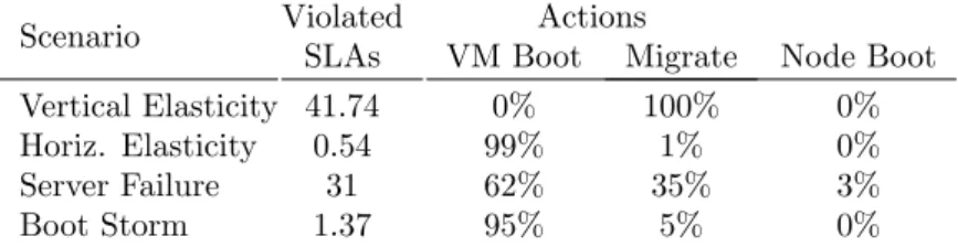
Scenario Violated Actions

SLAs VM Boot Migrate Node Boot Vertical Elasticity 41.74 0% 100% 0% Horiz. Elasticity 0.54 99% 1% 0% Server Failure 31 62% 35% 3%

Boot Storm 1.37 95% 5% 0%

Table 3.2: Violated SLAs and actions composing the reconfiguration plans. A SLA is failed when at least one among its constraints is violated. Table 3.2 sum-marizes the number of SLA failures and the distribution of the actions that composes the reconfiguration plans. We observe that the Vertical Elasticity and the Server Failurescenarios lead to the most violations. Furthermore, we observe a relation be-tween the number of migrations and the number of SLA violations. Initially, the current placement of the running VMs satisfies the constraints. During a reconfiguration, some VMs are migrated to their new hosts and once all the migrations are terminated, the resulting placement also satisfies the constraints. Until the reconfiguration is complete, a part of the VMs may be on their new hosts while the others are still waiting for be-ing migrated. This leads to an unanticipated combination of placements that was not under the control of the constraints. This explanation is also valid for constraints that manage the node state, such as maxOnlines. When the reconfiguration plan consists of booting VMs only, this situation cannot occur with the studied set of constraints. The placement constraints ignore non-running VMs and as each VM is deployed on a satisfying host, temporary violation is not possible.

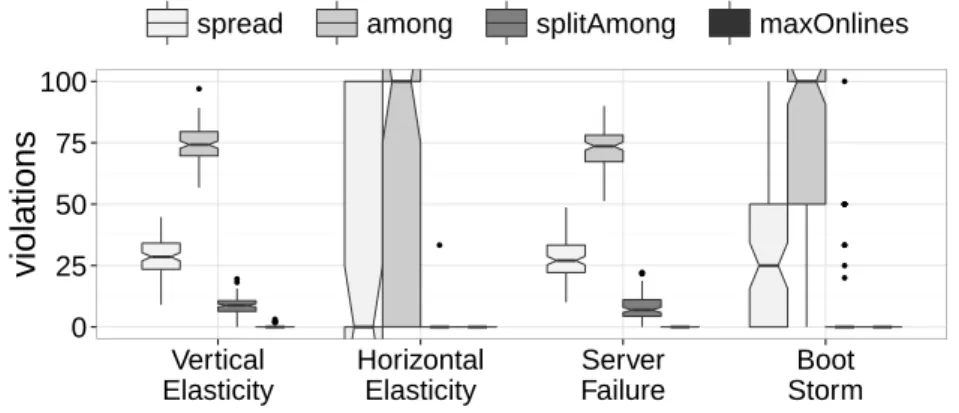
Distribution of the violated constraints

Figure 3.2 presents the average distribution of violated constraints in violated SLAs using box-and-whisker plots. The top and the bottom of each box denote the first and the third quartiles, respectively. The notch around a median indicates the 95% confidence interval. We observe among is the most violated constraint. Furthermore, with a distribution that exceeds 100%, multiple constraints can be violated within a single SLA. The violations are explained by the behavior of BtrPlace. To compute small reconfiguration plans, BtrPlace tries to keep each VM on its current node, otherwise, it chooses a new satisfying host randomly. If a VM involved in an among constraint must

● ● ● ● ● ● ● ● ● ● ● ● ● ● ● ● ● ● ● ● ● 0 25 50 75 100 Vertical Elasticity Horizontal Elasticity Server Failure Boot Storm violations

spread among splitAmong maxOnlines

Fig. 3.2: Distribution of the violated constraints

be migrated, BtrPlace has 94% chances to select a node on another rack, hence violating the constraint until the other involved VMs are relocated to this rack. This violation may reduce the performance of the application due to the slow interconnect between the VMs. For a VM subjects to a spread constraint, there is 2% chances at worst to select a node that already hosts a VM involved in the same constraint. The constraint will then be violated, leading to a potential single point of failure, until the other VM has been relocated elsewhere. For a VM subjects to a splitAmong constraint, the chances to select a node in the other cluster are 50% and the consequences of the resulting violation are similar to spread. Figure 3.2 reports more violation of spread than splitAmong constraints. There are 14 times more spread constraints so the chances to violate at least one constraint are higher.

The maxOnlines constraint has been violated 5 times, all in the vertical elasticity scenario. In these cases, the load increase saturated some racks. BtrPlace chose to boot the rack’ spare node to absorb the load and to shutdown a node in a non-saturated rack in exchange to satisfy the constraint at the end of the reconfiguration. BtrPlace schedules the actions as soon as possible. It then decided to boot the spare node before shutting down the other node which lead to a temporary violation of the constraint. With floating hypervisor licenses, this would lead to a non-applicable reconfiguration plan. The singleResourceCapacity constraint was never violated: BtrPlace schedules the VM migrations before increasing their resource allocation, it is then not possible to have a resource consumption that exceeds the host capacity.

Conclusion on discrete constraints

This experiment reveals temporary violations occur in BtrPlace despite the usage of placement constraints. We also discussed in Chapter 2 that other placement algo-rithms [29, 5] may also compute plans leading to temporary violations. Their cause is only related to the lack of controls over the computation of the actions schedule.

The consequences of these violations depend on the application requirements. For the applications that require high availability, the temporary violation of spread and spli-tAmongconstraints can lead to the unavailable of services in case the VMs co-allocate in the same node and the node fails. The applications that require high performance may experience degradation in performance if the VMs involved in the among constraint are not co-allocated. Similarly, the node performance may have bottlenecks if the hypervi-sors do not have enough resources. Finally, meeting license restriction is important for the datacenter as every single license violation costs an amount of money.

In the next chapter, we present continuous constraints that help to prevent the tempo-rary violations during the reconfiguration. The continuous constraints control not only the placement of VMs but also the action schedule.

Chapter 4

Elimination of Temporary

Violations with Continuous

Constraints

Depending on the users expectations, they may require the permanent satisfaction of the application requirements. In this chapter, we propose continuous constraints to con-trol the VM placement and action schedule guaranteeing the satisfaction of constraints continuously. We discuss the implementation and evaluation of continuous constraints whose discrete correspondences are previously evaluated in section 3.2.

4.1

Continuous constraint

A continuous constraint is a VM placement constraint that imposes the satisfaction of the constraint not only on the destination configuration but also during the recon-figuration. Continuous constraints can be used for critical application and datacenter requirements to ensure their satisfaction at any moment of the reconfiguration.

The implementation of continuous constraints requires a new look on the restrictions to express. To implement a discrete constraint, a developer only pays attention to the future placement of the VMs and the next state of the nodes. To implement continuous constraints, he also has to integrate the schedule of the associated actions. A pure placement problem in discrete constraints becomes a scheduling problem that is harder to tackle in continuous constraints.

BtrPlace already exposes not only variables related to the VM placement and node state at the end of the reconfiguration, but also variables related to the action schedule. We have implemented the continuous constraints by extending the discrete ones to act, when necessary, on the action schedule.

4.2

Modeling the continuous constraints

Different constraints have different level of difficulty. Some constraints, like among and splitAmong, do not require the action schedule to implement their continuous restric-tion. Other constraints need to take into consider the order of actions’ execution to achieve the continuous satisfaction.

The continuous implementation of among and splitAmong does not need to manipulate the action schedule. If a VM is already running on a node, the continuous implementa-tion just restricts the VM placement to the associated group.

The continuous implementation of spread prevents the VMs from overlapping. In practice, when a VM is migrated to a node hosting another VM involved in the same constraint, we force the start time of the migration action to be greater or equal to the variable denoting the moment the other VM will leave the node.

Other constraints are much more complex than the implementation of spread con-straints which simply restricts the start and the end moments of migrations. In the next subsections, we compare the discrete and continuous restriction of the constraints that I have developed in the thesis.

4.2.1

MaxOnlines

The definition and practical interest of MaxOnlines constraint are presented in sec-tion 3.1.

Discrete restriction The discrete implementation of maxOnlines extracts the boolean variables that indicate if the nodes must be online at the end of the reconfiguration and forces their sum to be at most equal to the given amount (4.1).

card(nq_j = 1) ≤ K, ∀nj ∈ N , j ∈ S (4.1)

Continuous restriction For a continuous implementation, we model the online pe-riods of the nodes and guarantee that their overlapping never exceeds the limit K. Because BtrPlace does not provide variables to model the online period of a node, we have then defined this period from pre-existing variables related to the scheduling of the potential node action.

We defined ps

i and pei in equation (4.2) as the moments a node i becomes online or

offline, respectively. These two variables are declared in the Power-Time View and are injected in the Reconfiguration Problem. If the node is already online, figure 4.1(a), ps i

equals the reconfiguration start and pe

i equals to the sum of the hosting end moment

S ps as_he _ae_pe _rpe ps as_ae _pe _he_rpe ad

time

(a) Shutdownable action

ps as _ae _pe_he rpe ps as_ae _pe_he _rpe ad B

time

(b) Bootable action

Fig. 4.1: Modeling Power-Start and Power-End of a node

online, the shutdown action is not executed and the variables as_{, a}d_{, a}e_{all equal to 0. As}

a result, ps

i equals 0, and pei equals he, equivalent to rpe, the end of the reconfiguration.

Otherwise, if the node is offline at first, figure 4.1(b), ps

i equals the action start and pei

equals the hosting end moment he _{of node i. In case of the node staying offline during}

the reconfiguration, the boot action is not executed, and as a consequence, ps

i and pei

are equal to 0. The online period for the node i is then defined with a time interval bounded by ps

i and pei. We finally restrict the overlap of the online periods as follow:

N1

N2

N3

time

N1

N2

N3

S

B

ps _pe _rpe 2 2 p s 3 p e 3 pe 1 ps1

Fig. 4.2: Cumulative scheduling of maxOnlines constraint

card({i|ps

i ≤ t ≤ pei}) ≤ K, ∀t ∈ T (4.2)

This restriction can be implemented as a cumulative constraint[42], available in Choco [37], the CP solver used in BtrPlace. Cumulative is a common scheduling constraint that restricts the overlapping of tasks that have to be executed on a resource. Figure 4.2

depicts a cumulative scheduling of a maxOnlines constraint which only allows 2 nodes online simultaneously.

4.2.2

MinSpareNode(S, K) & MaxSpareNode(S, K)

MinSpareNodeand MaxSpareNode manage the maximum and minimum number of spare nodes in the node set S (S ⊂ N ), respectively. A spare node is a node is online and idle (do not host any VM) to be available for VM provision when there is a load peak. A node provides the resources as coarse-grain, so it is easier to control the resources at the node level. The practical interest of minSpareNode is reserving a specific number of spare nodes to deal with application load spike whist the practical of maxSpareNode is restricting the number of spare nodes to use the power efficiently.

card({nq_j = 1 ∧ nvm

j = 0}) ≥ K, ∀nj ∈ S (4.3)

Discrete restriction In equation (4.3), a spare node is modeled as a node is being online and not hosting any VM. For minSpareNode constraints, the cardinality of the spare nodes in the set S has to be greater or equals to the constant number K indicated in the constraint. In the opposite, this number has to be less than or equals to K in maxSpareNodeconstraints.

i

e

time

VM1 VM2 VM1 VM2

i

e

i

s

i

s

rp

e B

N1

N2

Fig. 4.3: Modeling idle period of a node

continuous restriction Similar to the online period of a node, the idle period is not defined yet in BtrPlace. A node is in the spare period if it is online and does not host any VM. We define idle-start and idle-end (is _{and i}e _{in figure 4.3) to indicate the moment}

of the node becomes idle and occupied, respectively. If the node is already online, the idle-start equals to the moment of the c-slice that leaves the node last. On the other hand, if the node is offline at the beginning, the idle-start equals to the hosting-start of the node. The idle-end of the node equals to the moment of the d-slice that arrives the node first. If no VM arrives on the node, the idle-end equals to the hosting-end of that node. The idle period of a node then equals to the period between the idle-start and idle-end.

idle-starti = ( M AX(ce_{) if n}q i = 1, hs _{if n}q i = 0. (4.4) idle-endi = ( M IN (ds_{) if n}q i = 1, he _{if n}q i = 0. (4.5)

M inSN : K ≤ card({i|idle-starti ≤ t ≤ idle-endi}) ≤ N , ∀t ∈ T (4.6)

M axSN : 0 ≤ card({i|idle-starti ≤ t ≤ idle-endi}) ≤ K, ∀t ∈ T (4.7)

The Cumulative constraint is used to prevent the limit of the number of spare nodes during the reconfiguration. The node idle-start is identical to the the task start. A node idle period is identical to the task duration. The limitation is the capacity of the resources. The Cumulative constraint has a variable of minimum consumption of resources. In this model, the minimum consumption variable is identical to the minimum of idle nodes. Then for MinSpareNode constraint, we set the minimum consumption variable to the number K and the capacity variable to the total number of nodes involved in the constraint. On the other hand, the minimum consumption can be zero, and the capacity equals to K in MaxSpareNode constraint.

4.2.3

MinSpareResource(S, r, K)

The MinSpareResource constraint reserves at least a specified number K of idle re-sources r directly available for VM provision on the set of node S (S ⊂ N ). The practical interest of the constraint is preventing the nodes from saturation whenever a load spike occurs. Turning on a node or migrating a VM out of the saturated node may take long time, leading to some certain performance degradation of applications. The MinSpareResource constraint is used in this situation to keep an amount of idle resources to absorb the load spike.

X j∈S nq_jnr j − X dr i ≥ K, ∀d ∈ D, d h i = j (4.8)

Discrete restriction The model of MinSpareResource is represented in equation (4.8). The number of spare resources equals to the difference of the capacities to the sum of allocated resources. The resource r can be CPU, memory, etc. The number of spare re-sources has to be greater or equal to the constant number K indicated in the constraint.

X j∈S nq_jnr j− X ∀c∈C ch i=j cr i − X ∀d∈D dh i=j dr i ≥ K, ∀t ∈ T , d s i ≤ t ≤ c e i (4.9)

Continuous restriction BtrPlace provides an adapted Cumulative constraint to schedule fine-grain resources. The Cumulative constraint takes the inputs including resource capacity, arrays of c-slice and d-slice of VMs and node indexes. This constraint ensures the cumulative usage of c-slices and d-slices does not exceed the capacity of each node and the cumulative capacity specified in the constraint. In the equation (4.9), the number of spare resources equals to the difference between the capacity of nodes and the usage of c-slices that have not leave their hosts and d-slices that arrived on the new hosts. By extending the Cumulative constraint, the MinSpareResource constraint ensures the number of spare resources is continuously reserved during the reconfiguration.

The continuous implementation of maxOnlines, minSpareNode, maxSpareNode and minSpareResourcesappeared then to be more challenging than the implementation of spread, among and splitAmong. The developer must have a deeper understanding of the node actions to model their online period. For an efficient implementation, he must also understand how his problem can be expressed using pre-existing constraints.

4.3

Trade-off between reliability and computability

In this section, we present the preliminary results of the implementation in order to provide the continuous satisfaction of the constraints. The results show the continu-ous constraints have prevented the temporary violations during the reconfiguration of datacenters. Nevertheless, the result also exhibit obstacles of continuous constraints in computing the viable configuration.

4.3.1

Reliability of continuous constraints

Vertical Elasticity Horizontal Elasticity Server Failure Boot Storm Solv ed instances 0 20 40 60 80 100 Discrete, 1 min. Continuous, 1 min. Discrete, 5 min. Continuous, 5 min.

Fig. 4.4: Solved instances depending on the restriction.

We evaluate here the reliability and computational overhead of continuous constraints with regards to their discrete correspondence on the simulator presented in Section3.2. Each instance has been solved with a timeout set to 1 then 5 minutes to be able to qualify the difficulty of the instances.

Figure 4.4 and 4.5 present the number of instances solved by BtrPlace depending on the restriction and the average solving duration, respectively. As expected, none of the plans computed using continuous constraints leads to a temporary violation. With only discrete constraints, BtrPlace solved 95% of the instances within 1 minute and 100% of them within the 5 minutes. When using only continuous constraints, BtrPlace can solve 68% of the instances with 1 minute timeout. Increasing the timeout to 5 minutes helps BtrPlace at computing solutions for the Boot Storm and the Server Failure scenarios. The number of solved instances increases to 85.25% for 5 minutes timeout. Finally, to check the failed cases whether they are solvable, the timeout value is set to one hour. Then BtrPlace found a solution for 95.5% of the instances.

The continuous constraints put more restrictions on placement algorithm to find a sched-ule that satisfies the constraints at all the time. These restrictions increase the

com-plexity of the algorithm to find the solution. Some instances that are higher in initial workload are more complex to find a solution than the other instances. This circum-stance increases the time for the algorithm to the solution. The more timeout the placement algorithm has, the more number of instances can be solved.

4.3.2

Computational overheads for continuous constraints

The additional restrictions provided by the continuous constraints may impact the per-formance of the underlying placement algorithm. The overhead of the continuous con-straints is explained by their additional computations to disallow temporary violations. This overhead is acceptable for the Vertical Elasticity and Horizontal Elastic-ity scenarios with regards to their benefits in terms of reliability as the computation duration in these scenarios just increases a couple of seconds.

Vertical Elasticity Horizontal Elasticity Server Failure Boot Storm Solving dur ation (seconds) 0 10 20 30

40 Discrete, 1 min._{Continuous, 1 min.}

Discrete, 5 min. Continuous, 5 min.

Fig. 4.5: Solving duration depending on the restriction.

For the Boot Storm and the Server Failure scenarios, the overhead is more important. BtrPlace was not able to solve 30 instances within the allotted 5 minutes. This confirms these classes of problems are much more complex to solve. With the timeout set to 5 minutes, we observe a high standard deviation. This reveals a few instances are very hard to solve within a reasonable duration. Comparing these hard instances with the others may exhibit performance bottlenecks and demand for optimizing the implementation of continuous constraints. We are currently studying the remaining unsolved instances but we think some of these instances cannot be solved without a relaxation of the continuous component of some constraints.

Although, continuous constraints prevent the temporary violations of SLAs during data-center reconfiguration, they also increase the computational overheads for the placement algorithm to find a solution. The viable reconfiguration plan sometimes cannot be found within a certain amount of time. Then a possible solution is providing users a tool to characterize the constraint tolerance.

Chapter 5

Conclusion

Cloud computing offers the opportunities to host applications in virtualized datancenters to reduce the deployment costs for customers and to utilize the hosting infrastructure effectively. The use of virtualization techniques provides the ability to consolidate several VMs on the same physical node, to resize a VM resources as needed and to migrate VM across network for server maintenance. The primary challenge for cloud providers is automatically managing their datacenters while taking into account customers’ SLAs and resource management costs.

In a virtualized datacenter, customers express their SLAs through placement constraints. A VM placement algorithm is then in charge of placing the VMs on the nodes according to the constraints stated in the customer SLAs. Usually, a constraint manages the VM placement only at the end of the reconfiguration process and ignores the datacenter intermediary states between the beginning and the end of the reconfiguration process. We defined this type of constraints is the discrete placement constraint.

Through simulating datacenter reconfiguration, we showed the discrete constraints are not sufficient to satisfy the SLAs continuously. The VM placement algorithm does not take into account of actions schedule and this approach may indeed lead to temporary violations. We exhibited these violations through BtrPlace, one of the placement algo-rithms that rely on discrete placement constraints. We observed the violations occur when a reconfiguration plan aims at fixing a resource contention of the VMs or resource fragmentation using migrations without action scheduling.

This thesis addresses the problem of placement algorithms relying discrete constraints. We proposed continuous constraints to satiate the SLA satisfaction by scheduling the actions in the reconfiguration. We modeled and implemented preliminary version of continuous constraints to prevent the temporary violations. The continuous constraints are evaluated with the same settings of their discrete correspondence. We asserted the continuous constraints improve the datacenter reliability by eliminating all observed temporary violations.

The implementation of the continuous constraints puts more challenges for the devel-opers. It first requires detailed understanding of the principles of a reconfiguration. It also transforms a supposed placement problem into a scheduling one which is harder to tackle. This means a developer has to study what are provided by the reconfigura-tion and which schedule and new variables he may need to use to achieve the goal of

continuous constraints.

Finally, the continuous constraints provide reliability for SLAs, but their computational complexity reduces significantly the scalability of the placement algorithm. Applications in load spikes may experience some degradation while the placement algorithm spends more time on finding a solution. We need to define the trade-off between reliability and performance of application for users to choose. Then the placement algorithm can enhance the computation by respecting the important constraints and ignoring the constraints that can stand with some transient failures.

Future Research

We want to investigate on the causes that can lead to temporary violations. Through observation, VM migration is the key contributor for these violations. Energy-efficient placement algorithms rely heavily on VM migrations. These algorithms are widely used and should be studied as they shall be subject to such violations. We also want to consider placement constraints that address new concerns, such as services dependency and automatic balancing, to investigate for their likelihood of being subject to violations, and for the consequences in case of violations.

We observed that continuous constraints impact the performance of a placement algo-rithm, while not being constantly required to deny temporary violations. We want then to explore the situations that make continuous placement constraints unnecessary and rely on a static analysis of the problems to detect these situations.

Finally, we noticed continuous constraints may lead to unsolvable problems. In this situation, a user may prefer a temporary violation of its SLA. This however implies to allow the users to characterize their tolerance. We want then to model the cost of a constraint violation and integrate this notion inside BtrPlace.