HAL Id: hal-02663616
https://hal.inrae.fr/hal-02663616
Submitted on 31 May 2020
HAL is a multi-disciplinary open access archive for the deposit and dissemination of sci-entific research documents, whether they are pub-lished or not. The documents may come from
L’archive ouverte pluridisciplinaire HAL, est destinée au dépôt et à la diffusion de documents scientifiques de niveau recherche, publiés ou non, émanant des établissements d’enseignement et de
Industry location and welfare when transport costs are
endogenous
Kristian Behrens, Carl Gaigné, Jacques-François Thisse
To cite this version:
Kristian Behrens, Carl Gaigné, Jacques-François Thisse. Industry location and welfare when trans-port costs are endogenous. Journal of Urban Economics, Elsevier, 2009, 65 (2), pp.195-208. �10.1016/j.jue.2008.11.003�. �hal-02663616�
Version postprint
Industry location and welfare when transport costs
are endogenous
Kristian Behrens
∗Carl Gaigné
†Jacques-François Thisse
‡November 10, 2008
Abstract
Although transport costs are a key-ingredient of New Economic Geography, the trans-port sector is usually abstracted away from the analysis. Put differently, freight rates are taken as parametric and are not set by the market. This paper studies the relationships between transport costs, industry location, and welfare when freight rates are set by profit-maximizing carriers. We show that the demand for transport services becomes less elastic as the degree of spatial agglomeration rises, which increases carriers’ market power and al-lows them to charge higher markups. Once it is recognized that firms and consumers are free to relocate in response to changes in transport costs, an increasing number of carriers, falling fixed or marginal costs in transportation, or both, trigger a gradual agglomeration of industry. In the long run, this leads to consumer welfare losses (and to aggregate welfare losses under free entry), with more inequality across agents living in different regions.
Keywords: transport sector; new economic geography; imperfect competition; trade
JEL Classification: F12; F16; R12; R48
∗Université du Québec à Montréal, Montréal, Canada; CIRPÉE, Canada; and CORE, Université catholique de
Louvain, Belgium. Email: behrens.kristian@uqam.ca
†Corresponding author: INRA, UMR1302, 4 Allée Bobierre, F-35000 Rennes, France. Email:
carl.gaigne@rennes.inra.fr
‡CORE, Université catholique de Louvain, Belgium; PSE, France; and CEPR. Email:
Version postprint
1
Introduction
The main message delivered by New Economic Geography (henceforth, NEG) is that changes in the costs of shipping goods have a critical impact on industry location and the spatial distribution of welfare.1 Given the central role assumed by transport costs in that literature, one might
expect that much attention has been devoted to modeling them carefully. Yet, this is not so since freight rates are taken as exogenously given parameters, which amounts to assuming that the market for transport services is either perfectly competitive, with a perfectly elastic supply; or fully regulated, with freight rates set exogenously. Neither of these two extreme interpretations provides reasonable approximations of real-world transportation. We show in this paper that this modeling strategy is not innocuous in that accounting explicitly for market-based prices for transport services leads to different conclusions regarding the impacts of endogenous transport costs on the spatial structure of the economy and on welfare.
Given the emphasis put in NEG on transport costs, we find it natural to model explicitly the transport sector and to study how carriers’ pricing strategies interact with manufacturing firms’ location decisions and prices to shape the space-economy. To be precise, without intro-ducing explicitly the transport sector, the existing literature does not account for the fact that the location of economic activity depends on carriers’ behaviour, which depends itself on the way manufacturing firms are distributed across space as the latter influences interregional trade flows and, thereby, the demand for transport services. These two-way interactions between transport costs and the spatial distribution of economic activity must be analyzed within a full-fledged gen-eral equilibrium framework where locations, prices and freight rates are endogenously determined by market mechanisms. Although some recent NEG contributions deal with specific aspects of transportation, they all fall short of explicitly tackling the formation of prices in transport mar-kets.2 Filling this gap is the first objective of this paper and requires to make clear how freight
rates are determined by the transport sector.3
In addition, recent empirical evidence suggests that market structure in the transport sector
1See Fujita et al. (1999), Fujita and Thisse (2002), Baldwin et al. (2003) and Combes et al. (2008).
2Behrens and Gaigné (2006) and Behrens et al. (2006) analyze the agglomeration process when trade costs vary
exogenously with the volume of haul (density economies). However, they do not consider carriers’ pricing policies as transport markets are absent from their analysis. Similarly, Takahashi (2006) studies the impact of economic geography on the adoption of transport technology. He does not consider, however, carriers’ profit-maximizing behavior since he deals with a monopoly that is constrained by average cost pricing. Furthermore, transport costs are exogenous for each type of technology and modeling the transport sector is sidestepped by relying on Samuelson’s iceberg transport cost.
3It is worth recalling here that Samuelson (1954) introduced the iceberg transport cost in trade theory in order
Version postprint
matters in determining freight rates to a greater extent than improvements in infrastructure (Combes and Lafourcade, 2005). In the same vein, the deregulation of the freight industry from the early 1980s on has abolished many entry barriers and led to an increase in the number of carriers. Such changes in market structure are bound to affect freight rates by altering the competitive environment and carriers’ costs for providing transport services. Resorting to an absentee transport sector, very much as are absentee landlords in urban economics, does not allow one to fully study the welfare implications of such policies. Here too, our analysis leads to unexpected results.
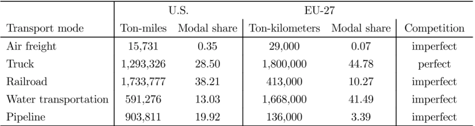
In this paper, we present a flexible model of the transport sector that can describe the market structure of different transport modes (trucking, rail roads, air freight and water transportation). Trucking, e.g., may reasonably be approximated by perfect competition in the wake of the Motor Carrier Act of 1980, which abolished most entry barriers and fare controls (Ying, 1990). That segment is characterized by a myriad of mostly small companies sharing the market and having little control over freight rates. On the contrary, railroads and water transportation are charac-terized by a small number of firms. Railroads are subject to high fixed costs as they require heavy infrastructure, thereby creating natural oligopolies. It is an industry with numerous barriers to entry, both natural and artificial, which explains why it has only a limited number of mostly large firms with market power.4 The shipping industry is characterized by a high degree of collusion (Sjostrom, 2004). Shipping conferences share the different shipping routes, set rates, and decide whether or not to accept new members by restricting entry. This industry is, therefore, clearly not competitive and should be more accurately described as a sector with restricted entry and significant economies of scale because of high fixed costs.
Insert Table 1 about here.
Table 1 provides some evidence on the structure of the transport sector in the U.S. and in the EU-27. As one can see, the share of the imperfectly competitive segments of the transport sector account for about more than 50% of ton-miles shipped in both cases, thus suggesting that a model including imperfect competition in transportation is warranted in modeling that sector in general equilibrium.5 This is what we undertake in this paper by providing a flexible model of the
4In the U.S., e.g., the “railroad industry is highly concentrated in the hands of seven railroads. Competition
is further limited by their geographical concentration [. . .] There are significant barriers to potential competitors entering the market, and this gives existing railroads pricing power. The industry also has relatively high fixed costs and exhibits increasing economies of scale" (Weatherford et al., 2008, p.23).
5While air freight is a sector that has been growing in importance for international transportation recently,
it is not a significant shipping mode at the regional level (see Table 1). Since the latter one is more relevant to the NEG framework we develop in this paper, as imbalances in the spatial distribution of industry are driven by
Version postprint
transport sector in which we can go all the way from constant returns and perfect competition, on the one end of the spectrum, to increasing returns and imperfect competition under both restricted and free entry, on the other end.
In addition to providing microeconomic underpinnings to the pricing of transport services, we also need to take into account the manufacturing firms’ reactions to the strategies selected by carriers. This is done with the help of a model of location and trade that allows for a de-tailed description of the pricing and locational choices made by manufacturing firms in response to carriers’ pricing policies. Specifically, we will use the linear model proposed by Ottaviano et al. (2002) because it captures directly the impact that changes in freight rates have on manufac-turing firms’ pricing strategies. It is also analytically tractable and amenable to precise welfare analysis, which is the second objective of this paper. Indeed, our market structure, where the demand for transport services depends on the spatial distribution of the manufacturing sector, which itself varies with the degree of competition between carriers through the level of freight rates, makes our model well suited to study how different transport policies affect the well-being of economic agents, especially consumers and carriers. We believe that providing a detailed wel-fare analysis of changes in the transport sector, when the location of industry is no longer taken as given, is a worthwhile exercise. The main reason is that the location of economic activity is indeed sensitive to changes in transport and trade costs, which are often targeted by competition and trade policies.6 Furthermore, it is well known that the spatial organization of the economy
has important welfare implications that differ across groups of agents and locations (Ottaviano and Thisse, 2002; Charlot et al., 2006, Gaigné, 2006). The welfare consequences triggered by changes in the spatial structure of the economy following investments in infrastructure or dereg-ulation policies in transportation should, therefore, be taken into account when assessing the long-run desirability of such policies.7 This has, to the best of our knowledge, not yet been done in economic geography and in public economics.
Our key results may be summarized as follows. First, we show that the demand for transport services depends on the spatial distribution of the manufacturing sector. Rather unexpectedly, this demand becomes less elastic as the degree of spatial agglomeration rises, which increases carriers’ market power and allows them to charge higher markups. Given constant marginal cost in the transport sector, freight rates unambiguously rise with the degree of spatial concentration of production. Second, and as a direct consequence of the previous result, we show that the
mobility across regions, we do not consider this sector in more detail henceforth.
6For example, Teixeira (2006) shows that better transport infrastructure has resulted in more spatial inequality
across the Portuguese regions.
7This is especially so for the European Union which is committed to a ‘regional cohesion objective’ as spelled
Version postprint
economy becomes gradually more agglomerated as the number of carriers increases, the marginal or the fixed costs in the transport sector falls, or both. The reason is that market power in the transport sector implies that more agglomeration raises freight rates for manufactured goods, thus dampening the agglomeration forces. In other words, the agglomeration process is self-defeating because of the stabilizing forces due to changes in freight rates. Finally, our results reveal some unsuspected long-run effects of changes in the market structure of the transport sector on welfare. Interestingly, they are all related to the spatial organization of the economy. When the dependence of the spatial distribution of production on the competitive environment in the transport sector is taken into account, more carriers and/or decreasing marginal or fixed costs in that sector lead to aggregate consumer welfare losses. Stated differently, while falling marginal costs and/or markups in the transport sector are beneficial to consumers when the spatial distribution of firms is fixed, the reverse holds true when the location of industry may change with transport costs. This result is shown to hold regardless of whether entry in the transport sector is restricted or free. In the latter case, as profits are zero in transportation at equilibrium, a decrease in marginal or in fixed costs unambiguously leads to social welfare losses. Hence, the short-run benefits of deregulation could well be offset by the long-run costs triggered by making the distribution of economic activity less efficient.8 Last, we show that transport deregulation may lead to higher
aggregate profits in that sector, and more inequality among consumers in different regions. It is worth stressing that these results are more than a mere theoretical curiosum and may have important policy implications that have been largely overlooked until now. It is thus fair to say that, from both the positive and normative viewpoints, the market structure that characterizes the freight industry has a strong impact on the space-economy, implying that the transport sector should become a fundamental building block of NEG models. It is also our contention that NEG offers a significant addition to public economic analyses on the impacts of policies that are bound to affect the spatial organization of the economy in the long run.
The remainder of the paper is organized as follows. Section 2 sets up the model and provides some preliminary results. The market outcome for the transport sector is analyzed in Section 3. In Section 4, we show how the degree of competition in the transport sector affects the location of the manufacturing sector and the volume of trade. Section 5 provides a detailed welfare analysis of the consequences of changes in market structure or the technology prevailing in the transport sector. Finally, Section 6 concludes.
8Likewise, but in a very different context, Norman and Thisse (1996) show that favoring a tough pricing policy
Version postprint
2
The model
The economy consists of two regions, labeled r or s = H, F . Variables associated with each region will be subscripted accordingly. There are two production factors, skilled and unskilled labor. We denote by L the total mass of skilled and by A the total mass of unskilled workers in the economy. Each individual works and consumes in the region she lives in. While the unskilled are immobile and their interregional distribution is exogenously given, skilled workers are mobile and their spatial distribution is endogenously determined. To control for any exogenous size advantage, we assume that the unskilled are evenly spread across the two regions, each of which hosts a mass A/2 of them. Let 0 ≤ λ ≤ 1 stand for the share of skilled workers living in region H. Without loss of generality, we may then restrict ourselves to the domain λ ≥ 1/2, i.e., agglomeration of mobile workers takes place in region H.
In order to disentangle the various effects at work, it is both relevant and convenient to distinguish between what we call a short-run equilibrium, in which skilled workers are supposed to be immobile, i.e. λ is exogenous; and a long-run equilibrium when they are mobile, i.e. λ is endogenously determined. This distinction is of particular importance when assessing the welfare changes triggered by lower freight rates, as shown in Section 5.
2.1
Preferences
All workers have the same preferences over a homogeneous good and a horizontally differentiated good, made available as a continuum of varieties. The utility is quasi-linear and the subutility over the set V (with measure n) of varieties is quadratic. Let VH (with measure nH) and VF (with
measure nF) denote the sets of varieties produced in regions H and F , respectively. A consumer
residing in region r then solves the following problem:
max qsr(v) Ur ≡ X s=H,F ∙ α Z Vs qsr(v)dv− β− γ 2 Z Vs [qsr(v)]2dv ¸ −γ 2 " X s=H,F Z Vs qsr(v)dv #2 +q0 s.t. X s=H,F Z Vs psr(v)qsr(v)dv + q0 = yr+ q0
where α > 0, β > γ > 0 are parameters (the condition β > γ implies that consumers have a preference for variety); qsr(v) and psr(v) are the quantity and the consumer price of variety v in
region r when it is produced in region s; and yr is the consumer’s income, which depends on her
skilled or unskilled status. Although quasi-linear preferences rank far behind homothetic prefer-ences in general equilibrium models of trade and geography, Dinopoulos et al. (2007, p.22) show that “quasi-linear preferences behave reasonably well in general-equilibrium settings”. Besides
Version postprint
making the model analytically tractable, this assumption will also allow us (i) to avoid making ad hoc assumptions on the location of the transport sector (see section 2.3) and (ii) to conduct a truthful welfare analysis (see section 5).
All workers are endowed with one unit of their labor type (skilled or unskilled) and q0 > 0 units of the homogeneous good, which is chosen as the numéraire. The initial endowment q0
is supposed to be large enough for the consumption of the numéraire to be strictly positive at the market outcome. This assumption aims at capturing the idea that both goods are essential. However, it eliminates the income effect in the demand for the differentiated good. Solving the consumption problem yields the following individual demand functions:
qsr(v) = a− (b + cn)psr(v) + cPr s, r = H, F (1)
where a ≡ αb, b ≡ 1/[β + (n − 1)γ] and c ≡ γb/(β − γ) are positive bundles of parameters, and where Pr ≡ Z Vr prr(v)dv + Z Vs psr(v)dv (2)
is the price index (i.e., the average price) of all varieties sold in region r = H, F . Through the price index, we will be able capture the main effects of price competition among firms.
2.2
The consumption goods sectors
There are two sectors producing consumption goods. The traditional sector supplies the homoge-neous good under perfect competition using unskilled labor as the only input of a constant-returns technology. The unit input requirement is set to one by choice of units. In the manufacturing sector, monopolistically competitive firms offer the horizontally differentiated good employing both factors under increasing returns to scale. Specifically, we assume that firms face a fixed requirement of φ > 0 units of skilled labor, whereas their marginal unskilled labor requirement is constant and set equal to zero without loss of generality.9 Given the foregoing assumptions,
skilled labor market clearing in each region implies that
nH =
λL
φ and nF =
(1− λ)L φ .
Shipping the homogeneous good is assumed to be costless, thus implying that its price is equalized across regions.10 This explains why that good is the natural choice for the numéraire.
9When the marginal unit input requirement m is strictly positive, what follows continues to hold true provided
that α is replaced by α − m in the demand functions (Ottaviano et al., 2002).
10This assumption is standard in most trade and economic geography models. Introducing positive trade costs
Version postprint
Consequently, in equilibrium the unskilled wage is equal to one in each region. By contrast, shipping the differentiated varieties is costly. Specifically, firms have to pay a freight rate of t > 0 units of the numéraire per unit of any variety transported between the two regions. Throughout the paper, we focus on the meaningful case in which the freight rate t is sufficiently low for inter-regional trade to be bilateral, regardless of the firm distribution λ. Because there is a continuum of firms, each one is negligible to the economy. It may thus accurately treat t as a parameter. Note, however, that this rate will be endogenously determined by profit-maximizing and imper-fectly competitive carriers, whereas it is considered as exogenous in standard economic geography and location models. Furthermore, the existence of transport costs in the manufacturing sector implies that trade no longer leads to the equalization of skilled wages between regions; they are also endogenous in our setting.
We assume that product markets are segmented and that labor markets are local. The first assumption means that each firm is free to price discriminate and to set a price specific to the region in which it sells its output (Engel and Rogers, 1996; Wolf, 2000; Haskel and Wolf, 2001). The second assumption means that no interregional commuting takes place. For skilled workers this implies that their wages may differ across regions; we denote by wr the skilled wage rate
prevailing in region r. As markets are segmented, firm v located in region r maximizes profits given by: πr(v) = prr(v)qrr(v) µ A 2 + φnr ¶ +£prs(v)− t ¤ qrs(v) µ A 2 + φns ¶ − φwr (3)
where prs(v) is the producer price of variety v produced in region r and sold in s 6= r. Because
skilled workers are geographically mobile, aggregate regional incomes and demands depend on their spatial distribution.
2.3
The transport sector
In Ottaviano et al. (2002), for each unit shipped of the differentiated good the producer has to pay a fixed and constant number τ > 0 units of the numéraire, regardless of the spatial structure of the economy. This assumption can be interpreted in two alternative ways. First, pricing in transport services is fully regulated, with freight rates t set exogenously at τ . Second, the transport sector is competitive and the supply of transport services is perfectly elastic, with marginal cost τ and zero fixed costs. As argued in the introduction, neither of these two interpretations strike us as providing particularly reasonable approximations of real-world transportation in general. In what follows, we hence depart from these scenarios and consider that the transport sector is not perfectly competitive and that it supplies a finite quantity of transport services. Specifically, this
Version postprint
sector is described by a number m of carriers that engage in Cournot competition and supply non-cooperatively a homogeneous transport service. As will become clear in what follows, we both consider the case where m is fixed (‘restricted entry’) and where it is determined by carriers’ zero-profit (free-entry) condition.
All carriers have access to the same technology which requires f ≥ 0 units of unskilled labor to enter the market and τ > 0 units of unskilled labor to ship one unit of the differentiated good between the two regions.11 Note that our model does not rule our the limit case where f = 0, i.e., there are constant returns to scale. When unskilled workers move between regions in transporting the differentiated good, we find it reasonable to assume that they do not consume local goods when they temporarily stay outside their region of origin. In that case, we reap the benefits of quasi-linear preferences since the locations of carriers and of the unskilled workers they employ, as well as their spatial ownership structure, have no impact on the demand for the differentiated good, hence on the demand for transport services. They, therefore, need not be specified in what follows.
The sectoral mobility of the unskilled between the traditional and the transport sector implies that carriers pay a wage equal to one, meaning that f and τ are respectively the fixed and marginal costs in the transport sector. Letting qkbe the volume of the differentiated good shipped by carrier
k = 1, 2, . . . , m and Q the total output of the transport sector, the profit function of carrier k is given by
ΠTk = [t(Q)− τ]qk− f.
The equilibrium market freight rate t(Q) is determined as in standard Cournot oligopoly by the Nash equilibrium among the carriers.12
Our setup of the transport sector is flexible enough to encompass most relevant cases. When there is free entry and constant returns (f = 0) we fall back on the standard NEG case where marginal cost pricing prevails, which may be viewed as a reasonable approximation of today’s trucking industry in the U.S. or the EU. As this case is already covered by NEG, we do not discuss it any further in what follows. When there is free entry and increasing returns (f > 0), we
11When carriers’ production costs are incurred in terms of skilled labor, the analysis becomes more involved.
This is because both the manufacturing and the transport sectors compete for skilled labor, so that the entry of a new carrier leads to a decrease in the total mass of varieties. The welfare effects then depend on the trade-off between transportation resource savings and consumers’ preference for variety.
12At equilibrium, profits are non-negative. Since it may be profitable to ship commodities, manufacturing
firms may want to transport themselves their products. In what follows, we disregard this possibility. Note that in the U.S., manufacturing consumed only $21,81 billion of in-house transportation, but $80,25 billion of for-hire transportation (Source: Bureau of Transport Statistics, BTS/98-TS/4R, April 1998). Hence, about 80% of transport costs incurred in manufacturing are of for-hire type.
Version postprint
approximate a market structure where there are fixed costs and, therefore, a limited number of carriers, but where entry exhausts all pure profits. This case may be viewed as one of a deregulated industry characterized by scale economies (as, e.g., increasingly rail cargo). Last, entry may be restricted for various reasons irrespective of the existence of fixed costs, which corresponds to the case where m if fixed.13 As should be clear from our discussion in the introduction, the
optimal modeling strategy would require to separate the different transport modes according to their market structure and then explicitly allow for modal choice across them. Doing so is, unfortunately, beyond the scope of our general equilibrium model. We hence stick to a simple structure of the transport sector that allows for an easy parametrization of the toughness of competition.
Before proceeding further, it is worth stressing which types of structural changes we consider in the transport sector in our model. As pointed out by Boylaud and Nicoletti (2001), the main changes in transportation in recent years are due to deregulation which has: (i) facilitated entry into the transport industry, i.e., increased m; and (ii) reduced variable production costs, i.e., decreased τ .14 In our Cournot setting increasing m or decreasing τ have the same qualitative
impact on the market outcome since all lead to lower freight rates, which is precisely the effect we want to capture. As will become clear later, since there is a negative one-to-one relationship between the free-entry number of carriers m∗ and the fixed costs f , we may also consider the impact that reducing f under free entry has on freight rates and the spatial distribution of economic activity.
3
Prices, wages, and freight rates
Formally, the short-run equilibrium is described by a sequential game, with the carriers being the leaders and the manufacturing firms the followers. In the first stage, carriers choose the quantities
13This is, e.g., the case in many developing countries, where there are numerous formal and informal government
controls for entry and operation in the transport sector. The case where f = 0 and entry is restricted approximates the U.S. trucking industry between 1935 and 1980. It corresponds to a situation where, even in the absence of increasing returns, the regulation of entry confers market power to the carriers and allows them to charge positive price-cost margins. The same holds true when there are both positive fixed costs and regulated entry.
14Note that cost reductions due to technological innovations always generate a welfare gain when λ is fixed.
However, it has been argued (both in the U.S. and the EU) that much of the cost saving that has led to reduced rates is due to lower pays to labor (Gómez-Ibáñez and Meyer, 1998; Combes and Lafourcade, 2005). According to Engel (1998, p.34), “Cost savings have been achieved largely at the expense of for-hire truckdrivers, whose real average hourly earnings [. . .] declined by 40 percent between 1978 and 1996, compared with a 13-percent decrease for all private sector workers."
Version postprint
of transport service they supply, whereas manufacturing firms choose their prices in the second stage of the game, taking the freight rate as given. In other words, when choosing how much service to supply, carriers anticipate the consequences of their strategies on the volume of trade between the two regions. However, when choosing their strategies, carriers do not account for the impact that they have on the spatial distribution of the manufacturing sector. Though peculiar, two reasons motivate our choice. First, taking this effect into account makes the formal analysis much more involved without adding any further insights. Second, as shown in Section 5.2.2, allowing for carriers to take into account how their supply of transport services affects the spatial distribution of economic activity would make our main results even stronger.
3.1
Prices and wages
All manufacturing firms maximize their profits (3) with respect to the prices prr(v) and prs(v)
in each market separately. For any given value of t, the first-order conditions yield the following profit-maximizing prices:
(i) intraregional prices:
prr(Pr) =
a + cPr
2(b + cn) (4)
(ii) interregional prices:
psr(Pr) = prr(Pr) +
t
2 s6= r. (5)
Since all firms in a region face the same price index, (4) and (5) show that they will set identical prices. We may hence alleviate notation by dropping the variety index v in what follows. Expres-sions (4) and (5) further show that the price a firm sets in region r depends on the price index Pr of this region, which depends itself on the prices set by all other firms. Because each firm is
negligible to the market, it chooses its optimal price by taking aggregate market conditions and wages as given. At the same time, aggregate market conditions must be consistent with firms’ optimal pricing decisions. Hence, the (Nash) equilibrium price index Pr∗ must satisfy the following
fixed point condition:
Pr∗ = nrprr(Pr∗) + nspsr(Pr∗). (6)
Under the assumption of bilateral trade between regions, the equilibrium prices can be found by first solving (6) for P∗
r, using expressions (4) and (5), and substituting back to obtain:
p∗rr = 2a + ctns 2(2b + cn) and p ∗ sr= p∗rr+ t 2. (7)
Substituting the equilibrium prices (4) and the price index (2) into the demands (1), the equilib-rium consumption levels can be expressed as follows:
Version postprint
(i) intraregional demands:
qrr∗ = a− bp∗rr+ cnt
2 = (b + cn)p
∗
rr (8)
(ii) interregional demands:
q∗sr= q∗rr−(b + cn)t
2 = (b + cn)(p
∗
sr− t). (9)
Thus, a higher freight rate t raises the demand for each local variety at the expense of imported varieties. In other words, carriers’ pricing decisions have a direct impact on trade patterns and the substitution effect decreases when varieties becomes more differentiated (i.e., when c decreases). We are now equipped to determine the conditions on t for trade to occur between the two regions at the equilibrium prices (q∗
sr > 0 or, equivalently, p∗sr > t). It can be readily verified that
t≤ min ½ 2a 2b + cnH , 2a 2b + cnF ¾
must hold for both interregional demands to be positive. Because the equilibrium prices depend on the firm distribution, the occurrence of interregional trade also depends on the spatial distribution of the industry (via nH and nF). The most stringent condition on t is obtained when λ = 1, since
when all firms are agglomerated the larger market is more competitive and, therefore, harder to penetrate from the outside. This yields the following trade feasibility condition:15
t < ttrade≡
2a
2b + cn (C1)
Turning finally to the labor market, the equilibrium wages of the skilled are such that all operating profits are absorbed by the wage bill, i.e. Πr(w∗r) = 0. Stated differently, firms bid
up wages for workers until no firm can profitably enter in or exit from the market. Substituting the equilibrium prices, as well as the equilibrium quantities (8) and (9) into the profits (3), and solving for the wages gives
wr∗ = b + cn φ "µ A 2 + φnr ¶ (p∗rr)2+ µ A 2 + φns ¶ µ p∗ss− t 2 ¶2# (10) for r = H, F .
3.2
Freight rates
The demand for transport services is given by the aggregate volume of trade between the two regions evaluated at the equilibrium prices (7).16 Some straightforward calculations show that
15To improve readability, we single out some frequently cited conditions involving structural parameters by
indexing the equation numbers with ‘C’.
16In the literature on general equilibrium with oligopolistic competition (Bonanno, 1990), this means that we
Version postprint
the total volume of trade is as follows:
Q(λ, t) = nH µ A 2 + nFφ ¶ qHF∗ + nF µ A 2 + nHφ ¶ qF H∗ = ρ0 + ρ2λ(1− λ)η − [ρ1+ ρ2λ(1− λ)]t. (11)
so that the price-elasticity of transport demand is positive and finite:
ε(λ, t) ≡ −∂Q ∂t t Q = [ρ1 + ρ2λ(1− λ)] t ρ0+ ρ2λ(1− λ)η − [ρ1+ ρ2λ(1− λ)]t (12)
where ρ0, ρ1, ρ2 and η are strictly positive bundles of parameters defined in Appendix A.1. They satisfy the inequality
ρ0− ηρ1 > 0. (C2) A sufficient condition for Q > 0 for all λ is that all interregional demands for the manufacturing good are positive, which holds true as long as condition (C1) is satisfied.
Hence, for a given firm distribution, the demand for transport services is a linear and downward sloping function of the freight rate. However, the transport demand varies in complex ways with the spatial distribution of firms. In particular, Q is not monotone in the degree of spatial concentration of the manufacturing sector. Indeed, for a given value of t, it increases in λ when t > η and decreases otherwise. This is because two opposite effects are at work. First, when region H hosts an increasing share of firms and skilled workers, the quantities imported of each variety produced in the other region (q∗
F H) and the number of imported varieties (nF) both shrink,
which tends to reduce the volume of trade. Second, more agglomeration in region H increases the quantities exported of each variety produced in region H (q∗
HF) as well as the number of exported
varieties (nH), which tends to increase trade. Despite those opposing effects, we can show that
the transport demand function displays an important property with respect to λ. Using (12) and (C2), it is readily verified that
∂ε(λ, t) ∂λ =
−(2λ − 1)(ρ0− ηρ1)tρ2
Q2 < 0 (13)
which implies that the price-elasticity ε of the transport demand falls as the degree of spatial concentration of the manufacturing sector rises. This turns out to be the unambiguous outcome of two opposite effects. On the one hand, more agglomeration decreases the intercept of the demand for transport services, thus raising the price-elasticity; on the other hand, the demand gets flatter, thereby lowering the price-elasticity. As the latter effect always dominates the former, the price elasticity falls when λ increases.
outcome of the second stage is described by a Walrasian equilibrium. When locations are exogenous, the function Q is then the so-called ‘objective’ demand of the carriers.
Version postprint
We may now describe the game played by the carriers. First, the inverse demand for transport services is readily obtained as follows:
t(Q) = ρ0+ ρ2λ(1− λ)η ρ1+ ρ2λ(1− λ)
− Q
ρ1+ ρ2λ(1− λ)
. (14)
The market clearing condition in the transport sector being Pkqk = Q, the profit of carrier k is
given by
ΠTk(qk, q−k) = [t (Q)− τ] qk− f
where q−k is the vector of strategies chosen by the carriers other than k. As the inverse demand (14) is linear, this game has a single Nash equilibrium in pure strategies. For any given λ, the equilibrium freight rate t∗ of the Cournot game is given by a unique and symmetric solution:
t∗(λ, m) = τ + ρ0+ ρ2λ(1− λ)η − [ρ1+ ρ2λ(1− λ)]τ
(m + 1) [ρ1+ ρ2λ(1− λ)] . (15) The first term in (15) is the carrier’s marginal cost, and the second the carrier’s markup. Note that m → ∞ implies t∗ = τ, as in Ottaviano et al. (2002).
Using (13), we have
dt∗(λ, m) dλ > 0
so that the equilibrium freight rate increases in λ over [1/2, 1] for a given number of carriers. The reason is that more agglomeration of firms in region H makes the transport demand less elastic, thus endowing the carriers with more market power, which in turn allows them to charge higher freight rates. Consequently, given the number of carriers, the equilibrium freight rate is maximum when the manufacturing sector is agglomerated in region H (λ = 1), and minimum when this sector is evenly dispersed between the two regions (λ = 1/2).
We can now determine the condition for which trade always occurs as well as the free-entry number of operating carriers. In Appendix A.2, we show that a sufficient conditions for t∗(λ) <
ttrade to hold and mark-ups to be positive, regardless of the spatial distribution λ, is given by
τ ≤ τtrade(m)≡
a(2bm− cn)
bm(2b + cn) (C3)
which we assume to hold in what follows. Observe that τtrade(m)is increasing in m, meaning that
the restrictions on carriers’ marginal cost for bilateral trade to occur gets less stringent as the number of carriers increases. The reason is that more competition in the transport sector leads to lower freight rates (provided the location of manufacturing firms is fixed), which hence favors the occurrence of interregional trade by increasing manufacturing firms’ ability to penetrate the foreign market.
Version postprint
Note also that when τ is large, the trade condition (C3) may be violated since the freight rates charged by the carriers are prohibitive. This is more likely to occur when the number of carriers is small, when goods are little differentiated, or both. In particular, it follows from (C3) that m > cn/2b must hold for interregional trade to occur. The interpretation of this condition is straightforward. When the manufacturing sector is very competitive (c or n is large) whereas the transport sector is not (m is small), an increase in freight rates makes the penetration of foreign markets almost impossible for exporters because local competition is too fierce.17 At the same
time, carriers must set a non-negative markup to break even. When τ is large compared to the preference for the differentiated good (captured by a), or when the differentiated goods market is very competitive, the demand for transportation services is small. In that case, carriers do not succeed to break even: on the one hand, they must set a freight rate larger than or equal to their marginal cost; on the other hand, there is no interregional trade at such a freight rate. In this case, the carriers set the lowest possible freight rate compatible with zero interregional trade, which is their profit-maximizing (loss-minimizing) strategy. Note that, in this case, transportation and trade between regions becomes asymmetric in the sense that only firms located in one of the two regions may export their varieties at the prevailing freight rate, whereas those located in the other serve only their local market.18
It remains to determine the free-entry outcome in the transport sector conditional upon the distribution λ. When the number of carriers becomes arbitrarily large, the equilibrium freight rate decreases and converges to marginal cost, so that profits also decrease and converge to zero. However, each firm entering the transport sector has to incur a positive fixed costs f . As a result, at the free-entry equilibrium, the number of carriers is finite and uniquely determined. Using, (15) and solving the zero-profit condition (t∗ − τ)Q(λ, t∗)/m− f = 0 with respect to m, yields the equilibrium number of carriers m∗(λ):19
m∗(λ) = ρ0+ ρ2λ(1p− λ)η − [ρ1+ ρ2λ(1− λ)]τ
f [ρ1+ ρ2λ(1− λ)] − 1. (16) As expected, the number of operating carriers decreases with the marginal and fixed costs. In addition, it is straightforward to check that
dt∗(λ, m∗(λ)) dλ = ∂t∗ ∂λ + ∂t∗ ∂m ∂m∗ ∂λ > 0.
In words, more agglomeration raises equilibrium freight rates even when the number of carriers
17Levin (1981, p.3) points out that “product market or “source” competition among shippers may constrain
[them] from raising the rates of [their] “captive shippers” for fear of pricing them out of the product market.”
18See Behrens (2005) for a more detailed analysis of asymmetric trade patterns in a similar framework. 19In what follows, we disregard the integer constraints on m∗.
Version postprint
is endogenously determined. This finding should not come as a surprise since the demand for transport services becomes less elastic when λ rises.
To summarize, we have shown the following result.
Proposition 1 When f > 0, the equilibrium freight rate increases with the degree of spatial concentration of the manufacturing sector, regardless of whether the number of carriers is fixed or whether entry is free.
Proposition 1 shows that it is worth to explicitly account for the transport sector in trade and geography models. Indeed, these models typically assume that transport costs are exogenously given and independent of the spatial distribution of their customers (the manufacturing sector in our model). We will show below that neglecting the resulting interdependencies has important consequences when studying the relationship between freight rates, industry location, and welfare. For a given distribution λ, the short-run market equilibrium is defined by (7), (10) and (15).
4
Freight rates and industry location
As in most economic geography models (Krugman, 1991; Fujita et al., 1999), firms move together with their workers. Thus, to determine the long-run equilibrium of the manufacturing sector (when λ is endogenous), it is sufficient to study the migration of skilled workers. These workers migrate to the region offering them the highest utility level evaluated at the equilibrium prices (4) and at the equilibrium wages (10). As shown by Ottaviano et al. (2002), the welfare of a consumer/worker living in region r = H, F is given by the sum of her consumer surplus, generated by the consumption of the differentiated good, her wage, and her consumption of the homogenous good, each evaluated at the short-run market equilibrium:
Vr∗ = Sr∗+ w∗r+ q0 (17) where Sr∗ = a 2n 2b − a(nrp ∗ rr+ nsp∗sr) + b + cn 2 £ nr(p∗rr) 2+ n s(p∗sr) 2¤ − c 2(nrp ∗ rr+ nsp∗sr) 2 (18)
is the consumer surplus evaluated at the equilibrium prices. Because (17) holds whatever the value of t, any change in the structural parameters of the transport sector is channeled through S∗
r and wr∗ only.20
20Note that the initial endowment is fully reflected in the indirect utility, since its consumption yields at least a
utility of q0. Yet, changes in t change the consumption of the numéraire good, which is given by 1 + q0−nrqrr∗ p∗rr−
Version postprint
The utility differential driving the location choices of the skilled is given by
∆V∗(λ, m)≡ VH∗(λ, m)− VF∗(λ, m). (19)
Thus, a spatial equilibrium arises at: (i) λ∗ ∈ [1/2, 1] when ∆V∗(λ∗) = 0; or (ii) at λ∗ = 1
if ∆V∗(1) ≥ 0. Such an equilibrium always exists because V∗
r is a continuous function of λ.
An interior equilibrium is stable if and only if the slope of the indirect utility differential (19) is negative in a neighborhood of the equilibrium, i.e., ∂(∆V∗)/∂λ < 0 at λ = λ∗, whereas an
agglomerated equilibrium is stable whenever it exists.
Evaluating ∆V∗(λ)at (4), (5), and (10), the indirect utility differential becomes
∆V∗(λ, m) = n(b + cn) 2φ(2b + cn)2 µ λ− 1 2 ¶ t∗(λ) [−ε1t∗(λ) + ε2] (20)
where ε1 and ε2 are strictly positive bundles of parameters whose expressions are given in
Ap-pendix A.1. It is easy to check that
ε2− ηε1 > 0 (C4)
a condition that will be useful in the welfare analysis of Section 5.
We now discuss the different types of spatial equilibria that may arise in our model. To do so, we first consider the case of a given number of carriers (with 1 ≤ m ≤ m∗), i.e., entry is
restricted. We then turn to the case where there is free entry (m = m∗). As we will show, results
are little sensitive to whether entry is restricted or free.
(i) Full agglomeration The distribution λ∗ = 1 is a stable long-run equilibrium if and only if −ε1t∗(1) + ε2 > 0 or, equivalently, t∗(1) = ρ0 − τρ1 (m + 1)ρ1 + τ < ε2 ε1 ⇐⇒ τ < τs(m)≡ m + 1 m ε2 ε1 − a bm.
The threshold τs(m)is called the sustain point by analogy with the terminology used in standard
economic geography models (Fujita et al., 1999). Observe that for both the agglomerated and the dispersed configurations to arise as a spatial equilibrium when transport and/or trade costs vary, it must be that τs(m) < τtrade(m). Indeed, when τs(m) > τtrade(m), there is always agglomeration
under bilateral trade, a case that arises when A is sufficiently small. By contrast, τs(m) <
τtrade(m) when the mass A of unskilled workers exceeds some threshold value A, which itself
exceeds L. Under this condition, it can be shown that ∂τs(m)/∂m > 0. Hence, agglomeration is
Version postprint
(ii) Dispersion The distribution λ∗ = 1/2 is a stable long-run equilibrium if and only if ∂¡∆V∗¢/∂λ < 0when evaluated at λ∗ = 1/2, which yields the condition
t∗(1/2) = 4(ρ0− τρ1) + ρ2(η− τ) (m + 1)(4ρ1+ ρ2) + τ > ε2 ε1 ⇐⇒ τ > τb(m)≡ m + 1 m ε2 ε1 − 4a (4b + cn)m. The threshold τb(m)is called the break point. As in the foregoing, τb(m) < τ
trade(m)implies that
∂τb(m)/∂m > 0, which again holds when A is sufficiently large. Consequently, dispersion is more likely to occur when the transport sector is little competitive (m is small).
It follows from condition (C2) that
τb(m)− τs(m) = ρ0− ηρ1 m(4ρ1+ ρ2)ρ1
> 0
which implies that: (i) the spatial equilibrium is always unique (up to a permutation of regions); and (ii) there exists a range of τ -values for which stable partially agglomerated equilibria arise. The intuition is that the gradual concentration of the manufacturing sector in one region leads to an increase of the equilibrium freight rate by making the transport demand more inelastic, thus slowing down the agglomeration process. The range of τ -values for which interior equilibria arise shrinks with the number of carriers. It is worth stressing that the sustain point and the break point are identical when f → 0 and m → ∞, which implies a catastrophic change in the distribution of firms (Ottaviano et al., 2002).
(iii) Partial agglomeration As shown in the foregoing, the economy may involve partial agglomeration of the manufacturing sector (1/2 < λ∗ < 1), which occurs when τb(m) > τ > τs(m). The equilibrium distribution λ satisfies the equation −ε1t∗(λ) + ε2 = 0, which is quadratic
in λ with two solutions symmetric about 1/2. The equilibrium value of λ > 1/2 is then given by
λ∗(τ , m) = 1 2+ 1 2 r Λ1 Λ2 (21)
where Λ1 and Λ2 are bundles of parameters defined in Appendix A.1. It is readily verified that
λ∗ < 1 when τ > τs(m) and that λ∗ > 1/2 when τ < τb(m).21 Therefore, 1/2 < λ∗(τ , m) < 1 if
and only if τb(m) > τ > τs(m). Furthermore, we have
∂(∆V∗) ∂λ ¯ ¯ λ=λ∗= −ε2Λ1(Λ2/ρ2) 2(m + 1)ε2 1(ρ0 − ηρ1)
which, under condition (C2), implies that the foregoing equilibrium is stable whenever τb(m) > τ > τs(m). Finally, we obtain sgn ∙ ∂λ∗ ∂m ¸ =sgn ∙ 4ε1(ρ0 − ηρ1)(ε2− ε1τ ) ρ2[(m + 1)ε2− ε1(η + mτ )]2 ¸ > 0 21Note that Λ
Version postprint
where the inequality comes from (C2). Given that firms price above marginal cost, and under (C3), the following condition holds at any interior equilibrium:
τ < ε2 ε1
= t∗(λ∗). (C5)
Hence, as the number of carriers rises, the economy moves gradually from dispersion to agglom-eration. Indeed, when some firms leave region F , say, toward region H, the equilibrium freight rate increases so that firms located in region F have an incentive to stay put because this allows them to relax price competition and to benefit from larger local demands since foreign firms face higher costs of exporting. Consequently, changes in the spatial organization of the economy are no longer catastrophic as agglomeration forces are now partially balanced by additional dispersion forces arising from the price-setting behavior in the transport sector. In other words, agglomera-tion becomes self-defeating, which stabilizes the spatial distribuagglomera-tion of firms. It is worth pointing out that such equilibria usually do not arise in standard core-periphery models with exogenous freight rates (Krugman, 1991; Ottaviano et al., 2002).22 Furthermore, when the transportation technology allows for very low marginal costs, we fall back on the standard result involving full ag-glomeration. Likewise, an increase in the number of carriers implies more agglomeration because competition in the transport sector is fiercer, hence facilitating the penetration of the smaller region from the larger one.
Insert Figure 1 about here
Accordingly, our findings, illustrated in Figure 1, can be summarized as follows.
Proposition 2 When the number of carriers increases, the spatial equilibrium gradually moves gradually from dispersion to full agglomeration of the manufacturing sector.
When the transport sector is oligopolistic, agglomeration emerges gradually because it in-creases carriers’ market power, thus introducing an additional incentive for the producers of the differentiated good to be dispersed.
(iv) Free entry in the transport sector Whereas in the foregoing cases m was taken as given, we now consider that entry is free. The equilibrium number of firms is then limited by the existence of fixed costs f > 0, and we may study the properties of the spatial equilibrium as f
22Puga (1999) and Pflüger (2004) are two noticeable exceptions. In the former model, agglomeration may be
self-defeating because it increases factor prices in the agglomerating region, whereas in the latter model the interaction between constant markups and quasi-linear preferences weakens the backward linkages due to expenditure shifting across regions.
Version postprint
gradually changes. To do so, we use (16) and (21) to derive the utility differential ∆V∗(λ, m∗(λ)),
which determines the equilibrium distribution of manufacturing firms under free entry in the transport sector. In what follows, we subscript variables pertaining to free entry with F .
Plugging (16) in (20) and repeating the arguments in (i)-(iii), we obtain the break and sustain points τbF ≡ ε2 ε1 − 2 s f 4ρ1+ ρ2 τ s F ≡ ε2 ε1 − s f ρ1 with τb
F > τsF. The equilibrium distribution of manufacturing firms is then given by λ∗F = 1/2
when τb F < τ, λ∗F = 1 when τ < τsF, and λ∗F = 1 2 + 1 2 s (4ρ1+ ρ2) ρ2 − 4f ε2 1 ρ2(ε2 − τε1) (22) when τb
F > τ > τsF. Clearly, λ∗F is decreasing in f . In words, transport technologies displaying
high scale economies (e.g., the railroad or airline industry), weaken the agglomeration forces once there is free entry in the transport sector. The reason is that high fixed costs allow for a small free entry number of carriers, which then charge high markups and foster dispersion.23 In contrast,
since the trucking industry seems to exhibit low scale economies (Ying, 1990), we may conclude that the growing use of trucks in shipping commodities may have fostered a larger concentration of activities.
In order to investigate the welfare impact of liberalization in the transport sector, we will consider below the following two thought experiments: (i) we treat m parametrically in order to track down the impact of carriers’ entry upon the distribution of manufacturing firms and (consumer) welfare and (ii) we study the consequences of free entry in the transport sector by endogenizing the number of carriers through the zero-profit condition.
5
Welfare analysis of changes in freight rates
We now turn to the second objective of this paper and ask whether deregulating the transport sector by facilitating entry is desirable from a welfare perspective. Deregulation is expected to promote a more efficient allocation of resources through fiercer competition between carriers, thus lowering freight rates and consumer prices (Morrison and Winston, 1999). Whereas count-less studies have investigated the welfare impacts of transport deregulation with a fixed spatial
23This interpretation is based on pricing only. One should keep in mind that high fixed cost industries usually
require localized infrastructure (hubs), which may serve to promote the agglomeration of industry. Furthermore, one may argue that there is a negative relationship between f and τ . As can be seen from (22), such a trade-off between f and τ has an ambiguous impact on the spatial equilibrium.
Version postprint
distribution of firms and demand, it is surprising that no study has yet, to the best of our knowl-edge, investigated these impacts by taking into account their spatial effects. This may be a serious issue since the very nature of transportation is spatial and since the bulk of the empirical evidence suggests that manufacturing firms’ locational decisions are still largely based on the accessibility to input and output markets (e.g., Head and Mayer, 2004; Redding and Venables, 2004). The major implication that has been very much overlooked in the literature until now is that transport policies affect not just consumer prices and the volume of commodity flows across regions, but also the location of industry. Since the location of economic activity directly affects freight rates via market mechanisms (see Section 3), and since the spatial structure of the economy has impor-tant welfare implications, a welfare analysis of transport deregulation with endogenous location decisions appears to be relevant.24
To investigate the welfare impacts of liberalization in the transport sector, we consider the following three thought experiments: (i) we treat m and λ parametrically and investigate the short-run impacts of changes in them on consumer prices and welfare; (ii) we treat m parametri-cally and λ endogenously in order to track down the long-run impact of carriers’ entry upon the distribution of manufacturing firms and welfare; and (iii) we study the consequences of free entry in the transport sector by endogenizing the number of carriers through the zero-profit condition. Since f and m∗ are monotonically linked by (16), all three exercises yield qualitatively similar results.
5.1
Exogenous industry distribution
Most economists and policy makers expect that more competition among carriers will decrease commodities prices because firms’ pay lower freight rates and because spatial price competition gets fiercer. When the location of firms is fixed, such a result obtains in our framework because
dPr∗ dm = ⎛ ⎝n∂p∗rr ∂t∗ + + ns 2 ⎞ ⎠∂t∗ ∂m − < 0
by using (2) and (7). Hence, when mobile factors do not relocate in response to changing freight rates, more competition in the transport sector unambiguously lowers the price indices of dif-ferentiated goods in both regions. Yet, this change does not directly map into a clear welfare assessment. Indeed, for a given value of λ, the impact of a lower freight rate on aggregate con-sumer welfare is a priori unclear. This is because of the interdependence between factor and
24See, e.g., Matsuyama and Takahashi (1998), Ottaviano and Thisse (2002), Charlot et al. (2006) and Gaigné
Version postprint
product markets, even when the location of firms is held fixed. Indeed, a decrease in t has two opposing effects: (i) it directly raises consumer surplus via lower prices, but (ii) it also indirectly lowers consumer welfare by triggering more competition on the products markets, thus leading firms to make lower operating profits and skilled workers to earn lower wages.
Standard, but tedious, calculations show that ∂W/∂t < 0 over the domain t < ttrade. In words,
for any given firm distribution, aggregate consumer welfare rises when freight rates decline even though wages decrease. As a result, we have
dW dm = ∂W ∂t − ∂t∗ ∂m − > 0. (23) Hence, we have:
Proposition 3 For any given firm distribution, increasing the number of carriers raises aggregate consumer surplus.
This result is in accordance with what transport analysts and policy-makers expect: transport deregulation makes consumers better off. Hence, even though wages fall, consumers always benefit from deregulation when the location of economic activity remains unchanged. The reason is that deregulation reduces freight rates and maps into lower consumer prices.25
5.2
Endogenous industry distribution
In what follows, we focus mainly on interior equilibria λ∗ ∈ (1/2, 1). Indeed, in the case of corner solutions (agglomeration or dispersion), the spatial distribution of firms does not change due to marginal changes in m. In that case, everything works as in the foregoing section with a fixed distribution.
5.2.1 Commodity prices
When the location of firms and skilled workers may change due to a fall in freight rates, our previous results no longer hold because both the slope and the intercept of the demand function (11) vary with λ. In particular, as shown in Appendix A.3, price indexes vary according to regions and in opposite directions:
dPH
dm =− dPF
dm < 0.
25This finding agrees with Morrison and Winston (1999) for whom a conservative estimate of the annual benefit
Version postprint
Observe that a marginal increase in m favors: (i) a fall in freight rates which, all else equal, reduces the prices of varieties consumed in both regions, as previously; and (ii) relocation of firms towards the large region. This gives rise to two opposite effects. On the one hand, for given freight rates, product prices decrease in the large region at the expense of the small one. On the other hand, more agglomeration implies higher freight rates (∂t∗/∂λ∗ > 0), as shown in Section 3, thereby raising product prices in both regions. It is hence not surprising that, as shown in Appendix A.4:
dp∗HH
dm < 0 and
dp∗F F
dm > 0.
In words, prices fall in the agglomerating region, whereas they rise in the region that loses firms despite the more competitive transport sector. These results may be summarized as follows.
Proposition 4 When the spatial equilibrium involves partial agglomeration, increasing the num-ber of carriers reduces commodity prices in the large region but raises them in the small one.
Hence, once we take into account the equilibrium relationship between agglomeration and freight rates, an increase in competition among carriers maps into lower consumer prices in the large region and higher consumer prices in the small one. Such a result suggests that the impact of transport deregulation could well be welfare-worsening, at least in one of the regions. This point is the focus of the next section.
5.2.2 Entry and consumer welfare
Our assumption of quasi-linear preferences allows us to define the aggregate consumer welfare as the sum of consumer surpluses and wages across individuals:
W (λ) = λL[S1∗(λ, t∗(λ)) + w∗1(λ, t∗(λ))] + (1− λ)L[S2∗(λ, t∗(λ)) + w2∗(λ, t∗(λ))]
+A 2[S
∗
1(λ, t∗(λ)) + S2∗(λ, t∗(λ)) + 2] + (A + L)q0. (24)
Differentiating W with respect to m yields dW dm = ∂W ∂t − ∂t∗ ∂m − +∂W ∂λ − ∂λ∗ ∂m + + ∂W ∂t − ∂t∗ ∂λ + ∂λ∗ ∂m + (25)
in which two additional terms appear when compared with (23). As a consequence, the first term in the RHS of (25) is always positive (as in the case where the spatial distribution of industry is fixed). The second term accounts for the impact of m on total welfare via a change in the spatial concentration of activities (at a given freight rate). We show in Appendix A.5 that, at a given freight rate, more agglomeration is welfare-decreasing (∂W/∂λ < 0). Indeed, when firms
Version postprint
and workers move, they do not take into account the benefits and losses they bring about to the agents residing in their new region, nor the benefits or losses they impose on those left behind. Hence, as in Ottaviano and Thisse (2002) who work with fixed freight rates, market forces yields too much agglomeration under partial agglomeration.26 The third term, which is specific to our
framework, captures the indirect effect that an increase in m has on the equilibrium freight rate, which impacts itself on the spatial equilibrium. This effect is negative because of our central result in Section 3: the more agglomerated the manufacturing industry, the less elastic its demand for transport services. Hence, ceteris paribus, the more agglomerated pattern triggered by the larger number of carriers raises the equilibrium freight rate, which in turn reduces total welfare. The two last terms in the RHS of (25) suggest that increasing the number of carriers could well be welfare-worsening since the entry of new carriers leads to more agglomeration.
Although the sign of (25) is a priori ambiguous, due to positive short-run gains and negative long-run losses, we show in Appendix A.6 that it may be signed unambiguously: dW/dm < 0. Hence, once it is recognized that firms and workers may change location in response to long run changes in competition between carriers, more competition in the transport sector can make consumers worse off because of excessive agglomeration.27 The spatial effects of transport
deregulation are at the heart of the explanation: a more competitive transport sector induces more agglomeration, hence raising freight rates and, thereby, reducing total welfare. We may thus conclude as follows:
Proposition 5 When the spatial equilibrium involves partial agglomeration, increasing the num-ber of carriers lowers aggregate consumers welfare.
The following two comments are in order. First, it is worth noting that our result also holds in the setting where carriers take into account how their supply of transport services affects the spatial distribution of industry. To see this, note that
dΠT k(qk, λ∗) dqk = ∂Π T k ∂qk + ∂Π T k ∂λ∗ ∂λ∗ ∂qk .
The first term is nil at the Nash equilibrium in the transport sector when firms disregard their impact on the spatial distribution of economic activity. As shown in Appendix A.8, in the second
26It is worth noting that the standard CES-iceberg model often yields too much agglomeration in equilibrium
(Charlot et al., 2006). Hence, our results cannot be dismissed on the basis that they are trivially driven by the tendency of excess agglomeration in the quadratic-linear setting.
27The entry of a larger number of carriers clearly leads to higher consumer welfare at the fully agglomerated
outcome than what it was under dispersion under regulation. However, as argued in the foregoing, full agglomer-ation does not strike us as a reasonable benchmark case against which to judge the welfare impacts of transport deregulation in the real world.
Version postprint
term, ∂ΠT
k/∂λ∗ is always positive at the quantity equilibrium when 1/2 < λ∗ < 1. This is because
the demand for transport services becomes more inelastic as the degree of agglomeration rises. Furthermore, ∂λ∗/∂qk is also positive since an increase in qk decreases t∗ which, as established
before, increases λ∗. Hence, when firms account for their impact on industry location, they further increase their supply of transport services, thereby sparking more agglomeration and reducing consumer welfare.
Second, transport policy also aims at enhancing technological efficiency by selecting the most efficient carriers, as well as by promoting a more flexible labor market and the adoption of new technologies. This should translate into lower costs and, in turn, lower freight rates and consumer prices. We can evaluate the impact of such a policy by studying the effect of a fall in marginal cost τ on consumer welfare. Standard calculations reveal that
dW dτ = dW dm m (ε2− ε1τ )ε1 > 0. (26)
For reasons similar to the ones mentioned above, a fall in carriers’ marginal cost favors the agglomeration of manufacturing firms, thus inducing higher freight rates and lower welfare.
Our result therefore suggests that there is a trade-off between short-run benefits and long-run losses: in the short long-run, a more competitive transport sector reduces static losses arising from market power in both the transport and the manufacturing sectors; but, in the long run, it generates dynamic dead-weight losses because of a sub-optimal redistribution of industrial activity across regions. In addition, as shown by (26), the harmful long run effects of deregulation may be offset by levying a tax on transportation that increases carriers’ marginal cost. Such a policy mix dominates pure deregulation because it can reduce welfare losses sparked by the redistribution of activities without having the baggage of limiting exit of inefficient firms and entry of efficient firms that regulation usually has.
5.2.3 Free entry and social welfare
Until now, we have only focused on aggregate consumer surplus. Strictly speaking, an accurate measure of social welfare must include the carriers’ aggregate profits. We hence now investigate how social welfare changes with the parameters of the transport sector in the free-entry equilibrium (m = m∗). Because profits are nil in both the manufacturing and transport sectors in such an equilibrium, W (λ) then provides a precise measure of social welfare in the whole economy. Under partial agglomeration, the free-entry equilibrium number of carriers is obtained by plugging (22) into (16), which yields:
m∗(λ∗F) =
(ρ0− ηρ1) + ε2
1f (η− τ)
Version postprint
We then clearly have dW dτ = dW dm dm∗(λ∗ F) dτ > 0 and dW df = dW dm dm∗(λ∗ F) df > 0.
In other words, a more efficient transport technology τ and lower entry barriers f have a negative long-run impact on social welfare. This surprising result stems from the fact that lower fixed and/or marginal transport costs foster entry, thereby leading to higher freight rates and lower total welfare as socially undesirable agglomeration takes place.
Proposition 6 When the spatial equilibrium involves partial agglomeration, any decrease in fixed costs f or variable costs τ lowers social welfare under free entry in the transport sector.
This result bears some resemblance with Ottaviano and Thisse (2002) who show that there is over-agglomeration when the transport sector operates under perfect competition and constant returns. They are not directly comparable, however. Freight rates are determined here through competition among carriers who face a demand schedule that varies with the distribution of the manufacturing sector, which itself depends the market freight rate. What we have is thus a full-fledged general equilibrium effect involving both the manufacturing and the transport sectors.
5.3
Individual consumer welfare and spatial equity
Until now, we have focused only upon the impact of liberalization in transportation on aggregate welfare. Yet, assessing more finely the individual changes across consumer groups is important because “regardless of economists’ explanations, the public is very sensitive to perceived changes in interpersonal equity” (Winston, 1993, p.1276). In our model, individuals living in different regions are affected differently by transport deregulation via changes in consumer prices and wages. Under full agglomeration or dispersion, we have seen that the welfare of any consumer increases when transport is deregulated. But how does individual welfare change when the economy involves partial agglomeration?
There are four types of consumers in our economy: skilled and unskilled workers, living in either region H or region F . Because unskilled workers are geographically immobile, and because their wage is fixed, all welfare changes materialize solely through consumer prices. Using (7) and (18), it is straightforward to check that:
dS∗ H dm = ∂S∗ H ∂pHH − ⎡ ⎣∂p∗HH ∂m − + 1 2 c 2b + cn ⎛ ⎝(1 − λ∗)∂t∗ ∂m − − t∗∂λ ∗ ∂m + ⎞ ⎠ ⎤ ⎦ > 0.