HAL Id: tel-01126872
https://pastel.archives-ouvertes.fr/tel-01126872
Submitted on 6 Mar 2015HAL is a multi-disciplinary open access
archive for the deposit and dissemination of sci-entific research documents, whether they are pub-lished or not. The documents may come from teaching and research institutions in France or abroad, or from public or private research centers.
L’archive ouverte pluridisciplinaire HAL, est destinée au dépôt et à la diffusion de documents scientifiques de niveau recherche, publiés ou non, émanant des établissements d’enseignement et de recherche français ou étrangers, des laboratoires publics ou privés.
MSPT : Motion Simulator for Proton Therapy
Paul Morel
To cite this version:
Paul Morel. MSPT : Motion Simulator for Proton Therapy. Autre [cs.OH]. Université Paris-Est, 2014. Français. �NNT : 2014PEST1094�. �tel-01126872�
Th`
ese
soumise pour obtenir le grade de
DOCTEUR DE L’UNIVERSIT ´
E PARIS-EST
MSPT : Motion Simulator for
Proton Therapy
Sous la direction de St´ephane Vialette et Xiaodong Wu. Sous l’encadrement de Guillaume Blin.
Sp´
ecialit´
e Informatique
´
Ecole doctorale MSTIC
Soutenue publiquement par Paul Morel
le 17 novembre 2014
Jury :
Guillaume BLIN
Universit´
e de Bordeaux
Examinateur
Pascal DESBARATS
Universit´
e de Bordeaux
Rapporteur
Serge MIGUET
Universit´
e Lumi`
ere Lyon 2
Rapporteur
Cyril NICAUD
Universit´
e Paris-Est
Pr´
esident
St´
ephane VIALETTE
Universit´
e Paris-Est
Directeur
Dongxu WANG
University of Iowa
Examinateur
Xiaodong WU
University of Iowa
Directeur
´
Ecole Doctorale MSTIC
Th`
ese de doctorat en informatique
MSPT: Motion Simulator for Proton
Therapy
Paul MOREL
Th`ese dirig´ee par St´ephane VIALETTE, co-dirig´ee par Xiaodong WU et co-encadr´ee par Guillaume BLIN.
Th`ese pr´epar´ee `a l’Universit´e Paris-Est Marne La Vall´ee, UMR CNRS 8049 LIGM, Bˆatiment Copernic, 5 boulevard Descartes, Cit´e Descartes, Champs Sur Marne,
`
A ma fille, Victoria et `a ma femme, Pauline.
Acknowledgments
MSPT: Motion Simulator for Proton Therapy
I thank Guillaume Blin1, St´ephane Vialette2 and Xiaodong Wu3,4, who jointly
super-vised my research during my PhD studies. They guided me and adsuper-vised me throughout my work to achieve my research on radiation therapy. I would like to express my grat-itude for the precious help of Dongxu Wang4, who played an important role during my
PhD. His advice throughout the development of MSPT, his clinical knowledge, his exper-tise in proton therapy and his help with all the simulations in RayStation have been a great support. I am grateful to Ryan Flynn4 and Edgar Gelover Reyes4 for their advice
and collaboration on the proton therapy project. I thank Daniel Hyer4, Yusung Kim4
and Christina Zacharatou5 for sharing and discussing about radiation therapy and proton therapy.
I express my thanks to Pascal Desbarats1, Serge Miguet6 and Cyril Nicaud2, members of my committee, for their time, their advice and their interest in my work.
I thank the members of the LIGM and the Universit´e Paris-Est Marne La Vall´ee for the three years spent together working and sharing good times.
I would like to acknowledge the financial support I received from the ANRduring my PhD: ANR project BIRDS JCJC SIMI 2-2010.
I express my gratitude to my family, Patrick, Th´er`ese, Pierre, Benoˆıt and Myriam, who nurtured my ambitions and my interest in engineering and in medicine since my young age. I also thank my family-in-law, Vanessa, Catherine, Alexandre, Sylvain, Marie-Fran¸coise, Marion, Etienne, and Quentin for their support, their advice and their thoughtful atten-tion since I know them. I also express my thanks to Vanessa, Pierre, Th´er`ese and Patrick for reading some parts of this thesis and helping me improve both my English and my French writing.
I thank all my friends, for all the moments we shared during these three years, which allowed me to unwind and to stop thinking about my thesis in order to get back to earth!
I wish to thank especially, Pauline, my wife, for her endless love and support, for the time she spent taking care of so many things while I was working on this thesis, for al-ways believing in me, for encouraging me surpass myself and for making my life happier. Finally, I would like to thank Victoria, our amazing daughter, for being such a source of joy and laugh.
1. LaBRI, Universit´e de Bordeaux (France)
2. LIGM, Universit´e Paris-Est Marne La Vall´ee (France)
3. Department of Electrical and Computer Engineering, University of Iowa (USA) 4. Department of Radiation Oncology, University of Iowa (USA)
5. Institut Bergoni´e, Bordeaux (France) 6. LIRIS, Universit´e Lumi`ere Lyon 2 (France)
MSPT: Motion Simulator for Proton Therapy
Abstract
In proton therapy, the delivery method named spot scanning, can provide a particu-larly efficient treatment in terms of tumor coverage and healthy tissues protection. The dosimetric benefits of proton therapy may be greatly degraded due to intra-fraction mo-tions. Hence, the study of mitigation or adaptive methods is necessary. For this purpose, we developed an open-source 4D dose computation and evaluation software, MSPT (Mo-tion Simulator for Proton Therapy), for the spot-scanning delivery technique. It aims at highlighting the impact of intra-fraction motions during a treatment delivery by comput-ing the dose distribution in the movcomput-ing patient. In addition, the use of MSPT allowed us to develop and propose a new motion mitigation strategy based on the adjustment of the beam’s weight when the proton beam is scanning across the tumor.
In photon therapy, a main concern for deliveries using a multileaf collimator (MLC) relies on finding a series of MLC configurations to deliver properly the treatment. The efficiency of such series is measured by the total beam-on time and the total setup time. In our work, we study the minimization of these efficiency criteria from an algorithmic point of view, for new variants of MLCs: the rotating MLC and the dual-layer MLC. In addition, we propose an approximation algorithm to find a series of configurations that minimizes the total beam-on time for the rotating MLC.
Keywords: Proton therapy, photon therapy, simulator, intra-fraction motions, mul-tileaf collimator decomposition.
R´
esum´
e
En proton th´erapie, la technique de balayage, permet de traiter efficacement le pa-tient vis `a vis de l’irradiation de la tumeur et la protection des tissus sains. Ces b´en´efices dosim´etriques peuvent cependant ˆetre grandement d´egrad´es par les mouvements intra-fraction. Par cons´equent, l’´etude de m´ethodes d’att´enuation ou d’adaptation est n´ecessaire. C’est pour cela, que nous avons d´evelopp´e un logiciel ”open-source” de calcul et d’´evaluation de dose en 4D, MSPT (Motion Simulator for Proton Therapy), pour la technique de ba-layage. Son but est de mettre en avant l’impact des mouvements intra-fraction en calculant la r´epartition de dose dans le patient. En outre, l’utilisation de MSPT nous a permis de mettre au point et de proposer une nouvelle m´ethode d’att´enuation du mouvement bas´ee sur l’ajustement du poids du faisceau quand celui-ci balaye la tumeur.
En photon th´erapie, un enjeu principal pour les traitements d´elivr´es `a l’aide de col-limateurs multilames (MLC) consiste `a trouver un ensemble de configurations du MLC permettant d’irradier correctement la tumeur. L’efficacit´e d’un tel ensemble se mesure par le total beam-on time et le total setup time. Dans notre ´etude, nous nous int´eressons `a la minimisation de ces crit`eres, d’un point de vue algorithmique, pour de nouvelles tech-nologies de MLC : le MLC rotatif et le MLC `a double couche. De plus, nous proposons un algorithme d’approximation pour trouver un ensemble de configurations minimisant le total beam-on time pour le MLC rotatif.
Mots cl´es : Proton th´erapie, photon th´erapie, simulateur, mouvements intra-fraction, d´ecomposition de collimateurs multilames.
R´
esum´
e fran¸
cais de la th`
ese
MSPT: Motion Simulator for Proton Therapy
La radiation th´erapie est un des traitements contre le cancer le plus utilis´e. Ce type de traitement peut ˆetre d´elivr´e de diff´erentes fa¸cons. Dans cette th`ese nous nous int´eressons `a une technique couramment utilis´ee appel´ee la photon th´erapie ainsi qu’`a la proton th´erapie qui reste peu utilis´ee mais qui suscite de plus en plus d’int´erˆet.
En proton th´erapie nous nous sommes int´eress´es au probl`eme du mouvement des patients pendant le traitement. Pour cela, nous avons d´evelopp´e un logiciel visant `a re-produire un traitement de proton th´erapie d´elivr´e `a un patient mobile. L’int´erˆet de ce simulateur est de rendre compte de l’impact du mouvement sur le traitement. D’autre part, il peut ˆetre utilis´e pour mettre au point des strat´egies ayant pour but de r´eduire l’impact de mouvement.
En marge de ce travail, nous nous sommes int´eress´es `a des probl`emes algorithmiques rencontr´es en photon th´erapie.
Dans une premi`ere partie nous introduirons le domaine de la radiation th´erapie et plus pr´ecis´ement : la photon th´erapie et la proton th´erapie. Nous introduirons ´egalement des probl`emes rencontr´es dans ces deux techniques. Dans une seconde partie nous pr´esenterons un logiciel d´evelopp´e pour faciliter l’´etude du mouvement en proton th´erapie. Enfin nous exposerons les r´esultats de l’´etude algorithmique r´ealis´ee en photon th´erapie.
Chapitre 1
Radiation th´
erapie
1.1
Pr´
esentation de la radiation th´
erapie
La radiation th´erapie est un traitement m´edical visant `a d´etruire des cellules canc´ereuses `
a l’aide de radiations ionisantes. Ce traitement est apparu en 1896, peu de temps apr`es la d´ecouverte des rayons X par le Dr. Roentgen (1895). Au fil du temps, cette technique a ´evolu´e pour donner naissance `a diff´erents proc´ed´es de radiation th´erapie utilis´es de nos jours : la curieth´erapie, la photon th´erapie et la proton th´erapie. La curieth´erapie, ap-partenant `a la radiation th´erapie interne, consiste `a ins´erer une source radioactive dans le patient afin de traiter la tumeur en pla¸cant cette source dans la tumeur ou `a proxi-mit´e de cette derni`ere. La photon th´erapie, appartenant `a la radiation th´erapie externe (voir Figure 1.1), utilise un rayon `a base de photons, dont l’´energie est sup´erieure `a 100 keV, et dont la source, situ´ee `a l’ext´erieur du patient, est orient´ee vers la tumeur. La proton th´erapie, appartenant ´egalement `a la radiation th´erapie externe, utilise un rayon de protons, dont l’´energie est situ´ee entre 30 et 230 MeV. Son principe est similaire `a celui de la photon th´erapie pour traiter un patient. Dans le cadre de cette th`ese nous nous int´eresserons `a la photon th´erapie et `a la proton th´erapie.
Figure 1.1 – Illustration de la radiation th´erapie externe : le faisceau de radiations ionisantes est externe au patient et peut tourner autour de ce dernier.
MSPT: Motion Simulator for Proton Therapy
1.2
Comparaison entre la photon et la proton th´
erapie
De nos jours, la photon th´erapie est un des traitements les plus utilis´es pour traiter les cancers. La proton th´erapie suscite de plus en plus d’int´erˆet de par le monde en raison des b´en´efices que cette technique apporte aux patients par rapport `a la photon th´erapie. En effet, la diff´erence majeure entre ces deux techniques est la quantit´e d’´energie d´epos´ee dans le corps du patient, appel´ee dose et mesur´ee en Gray (Gy), ainsi que sa r´epartition. Il est n´ecessaire de savoir que lors d’un traitement, on cherche `a d´eposer une dose tr`es im-portante au niveau de la tumeur, afin de tuer les cellules canc´ereuses, et de limiter autant que possible la dose re¸cue par les tissus sains dont les organes particuli`erement sensibles aux radiations appel´es organes `a risque (OAR). Limiter la dose re¸cue par les cellules saines est important afin de ne pas risquer de les tuer ou d’engendrer une d´eg´en´erescence de ces cellules qui pourrait conduire `a des tumeurs dites secondaires dont l’apparition peut se produire `a la suite d’un traitement `a base de radiations. En photon th´erapie le maximum de dose est d´epos´e rapidement apr`es la p´en´etration du rayon dans le patient, et la dose d´epos´ee d´ecroˆıt progressivement sans devenir nulle en traversant le corps du patient. En proton th´erapie, le maximum de dose est d´epos´e `a une certaine profondeur, appel´ee profondeur du pic de Bragg (Bragg Peak) d´ependant de l’´energie des protons. En aval de cette profondeur la dose d´epos´ee devient nulle. En amont de cette profondeur, la dose d´epos´ee est relativement faible. Si le rayon de protons contient des protons de diff´erentes ´energies (rayon poly-´energ´etique), il est possible d’observer plusieurs pics de Bragg, qui permettent de d´eposer une forte dose dans une ´epaisseur de tissus d´efinie, appel´ee la r´egion cible. La Figure 1.2, pr´esente un sch´ema de la dose d´epos´ee par des photons et des protons en fonction de la profondeur dans un certain milieu. La Figure
1.3, pr´esente la dose re¸cue par un patient par des rayons de photons et de protons.
Figure 1.2 – Profils de dose pour des photons et des protons.
MSPT: Motion Simulator for Proton Therapy
Figure 1.3 – Comparaison de la dose d´epos´ee dans un patient pour des photons (haut) et des protons (bas). [Kirsch and Tarbell, 2004]
Comme il est possible de le constater, l’utilisation de protons r´eduit consid´erablement la dose re¸cue par le patient. Malgr´e cela, la proton th´erapie n’est pas encore tr`es utilis´ee dans le monde. En effet, en Aoˆut 2013, seulement 43 centres de proton th´erapie ´etaient recens´es dans le monde, ce qui correspond `a 122 salles de traitement. Cela repr´esente 0.9% des centres de photon th´erapie [Goethals and Zimmermann, 2013]. Le principal facteur limitant le d´eveloppement de la proton th´erapie est le coˆut : environ 95 millions d’euros (≈ $130 millions) pour un centre de proton th´erapie et environ 23 millions d’euros (≈ $30 millions) pour un centre de photon th´erapie. De plus, le traitement d’un patient n´ecessite plusieurs s´eances d’irradiation, appel´ees fractions, dont le coˆut est d’environ 740 euros (≈ $1000) pour la proton th´erapie et d’environ 230 euros (≈ $300) pour la photon th´erapie [Peeters et al., 2010]. Petit `a petit les entreprises de proton th´erapie am´eliorent les technologies pour les rendre moins on´ereuses. Il est estim´e que d’ici 2030 le nombre de salles de traitement atteindra 1000 [Goethals and Zimmermann, 2013].
1.3
Des challenges en radiation th´
erapie
La photon th´erapie est d´elivr´ee `a l’aide d’un large faisceau de photons tournant autour du patient et auquel une forme est donn´ee afin de correspondre aux contours de la tumeur, `
a la dose minimale que doit recevoir la tumeur et la dose maximale qui ne doit pas ˆetre d´epass´ee pour les OARs. Cette conformation, en 2 dimensions, est accomplie `a l’aide d’un collimateur multilames (MLC). Un MLC est compos´e de paires de lames parall`eles pouvant bloquer ou laisser passer le faisceau (voir Figure 1.4). La planification du traitement consiste `a d´efinir une grille en 2 dimensions de la dose qui doit ˆetre d´elivr´ee localement au patient pour chaque angle du faisceau. Cette grille, appel´ee plan d’intensit´e, est r´ealis´ee par une s´equence de configurations du MLC. Bien que la qualit´e d’un plan de traitement soit jug´ee par des param`etres dosim´etriques, deux crit`eres permettent d’´evaluer son efficacit´e. Le premier crit`ere, appel´e total beam-on time, correspond `a la dur´ee totale de l’irradiation du patient. Il est ´egal `a la somme de la dur´ee de chaque configuration du MLC. Le second crit`ere, appel´e total setup time, repr´esente le temps n´ecessaire pour positionner les lames du MLC pour l’ensemble des configurations. Il est approximativement proportionnel au nombre de configurations. L’enjeu est de minimiser ces deux crit`eres afin d’avoir un
MSPT: Motion Simulator for Proton Therapy
plan efficace et de s’assurer que le patient ne re¸coit pas des radiations superflues ou un traitement prolong´e inutilement.
(a) Vue d’un Multileaf Collimator (MLC) dans le syst`eme utilis´e pour d´elivrer
le traitement. (b) Une configuration deMLC Figure 1.4 – Exemples deMLCs
Un traitement de proton th´erapie peut ˆetre d´elivr´e principalement de deux fa¸cons : la technique de diffusion ou la technique de balayage. La technique de diffusion est si-milaire au proc´ed´e utilis´e pour la photon th´erapie, c’est `a dire qu’un large faisceau est conform´e pour correspondre `a la forme de la tumeur. Cette technique, tr`es employ´ee de nos jours, commence `a laisser place `a la technique de balayage qui permet une meilleure pr´ecision pour irradier la tumeur et limiter les radiations inutiles re¸cues par le patient. Ce proc´ed´e emploie un faisceau mono-´energ´etique de protons tr`es fin (de l’ordre des quelques millim`etres) qui est balay´e sur l’ensemble de la tumeur. Le changement d’´energie des pro-tons, au cours du traitement, permet de modifier la profondeur o`u a lieu le balayage dans le patient en raison du pic de Bragg (voir Figure 1.5). Cette seconde m´ethode, bien que tr`es pr´ecise, est tr`es sensible aux mouvements du patient pendant l’irradiation. Ces mou-vements, qualifi´es d’intra-fraction, peuvent ˆetre d’origines diff´erentes comme par exemple : respiration, battements du cœur, toux, gaz intestinaux, ou le hoquet. Ces mouvements, peuvent entraˆıner de fortes d´egradations de la dose re¸cue par le patient. La Figure 1.6
pr´esente un exemple d’irradiation avec et sans mouvement.
MSPT: Motion Simulator for Proton Therapy
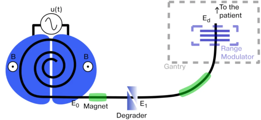
Figure 1.5 – Illustration de la technique de balayage. Pour chaque ´energie du faisceau de protons d´efinie dans le plan de traitement correspond une position du pic de Bragg (courbe
bleue). Une couche d’´energie correspond `a l’ensemble des points situ´es `a la profondeur du pic de Bragg. La position du faisceau est contrˆol´ee par un jeu d’aimants. A une ´energie et une position de faisceau correspond un poids qui repr´esente la dur´ee pendant laquelle l’irradiation de ce faisceau est maintenue.
Figure 1.6 – R´esultat de l’irradiation d’une plaque radiographique avec (droite) et sans (gauche) mouvements. [Paganetti et al.,2012]
Dans le cadre de cette th`ese nous aborderons le probl`eme de minimisation des crit`eres d’efficacit´e rencontr´es en photon th´erapie et le probl`eme de mouvements intra-fraction en proton th´erapie.
Chapitre 2
MSPT : Un simulateur de
mouvement pour la proton th´
erapie
2.1
D´
eveloppement d’un outil pour l’´
etude des
mou-vements intra-fraction.
Afin d’´etudier le probl`eme de mouvements intra-fraction en proton th´erapie nous avons d´evelopp´e un logiciel, appel´e MSPT (”Motion Simulator for Proton Therapy”). Ce simu-lateur est ”open source” et distribu´e sous la licence GNU GPL (v3). Le code source, la documentation et le manuel utilisateur peuvent ˆetre obtenus `a http://code.google. com/p/mspt/.
Le but principal de cet outil est de rendre compte de la r´epartition de dose dans le patient lors de mouvements intra-fraction pour un plan de traitement et un certain mouvement. Le second int´erˆet de MSPT est de fournir `a l’utilisateur des informations per-mettant de comparer diff´erents plans de traitement afin de pouvoir am´eliorer la robustesse du traitement pour ce patient vis `a vis des mouvements intra-fraction. Une technique de compensation de mouvement est ´egalement mise en œuvre dans MSPT, afin de proposer une strat´egie visant `a am´eliorer la robustesse des traitements en pr´esence de mouvements intra-fraction.
Ce simulateur a ´et´e d´evelopp´e en Python 2.7 et utilise des sous-routines en C pour am´eliorer la vitesse de traitement de certaines op´erations. Il re¸coit en entr´ee l’image CT (Computed Tomography) du patient, le plan de traitement (´energies des protons, posi-tions du faisceau pour le balayage et le poids de chaque position qui est ´equivalent `a une dur´ee), le contour des structures du patient (d´elimitation du corps du patient, d’organes et de la tumeur - voir Figure 2.1) et optionnellement la r´epartition de dose simul´ee dans un logiciel de planification de traitement. Toutes ces entr´ees utilisent le standard DICOM (Digital Imaging and Communication in Medicine). En outre l’utilisateur fournit un fichier de param´etrage du simulateur qui d´efinit son comportement ainsi que les mouvements du patient. MSPT fournit `a la fin de la simulation un ensemble de donn´ees permettant d’´evaluer la qualit´e du traitement aussi bien visuellement que quantitativement (voir exemple dans la Figure 2.2).
MSPT: Motion Simulator for Proton Therapy
Figure 2.1 – Exemple d’une image CT et de la repr´esentation de diff´erentes structures du patient : poumons (orange), r´egion cible comprenant la tumeur (rouge), moelle ´epini`ere (bleu) et des os de la colonne vert´ebrale (vert).
Figure 2.2 – Exemple d’une image CT et de la repr´esentation de la r´epartition de dose simul´ee dans MSPT.
2.2
Mod´
elisation
Le patient est repr´esent´e par des matrices 3D obtenues `a l’aide du CT. Plusieurs matrices sont utilis´ees pour repr´esenter la densit´e des tissus, leur pouvoir d’arrˆet, la pro-fondeur radiologique ainsi que le dose d´epos´ee. Pour calculer la dose d´epos´ee nous utilisons le mod`ele analytique propos´e parHong et al. [1996]. Ce mod`ele repose sur un calcul dans l’eau mis `a l’´echelle pour correspondre `a d’autres milieux. Nous avons dˆu ajouter `a ce mod`ele un facteur de correction de dose d´ependant de l’´energie et un facteur de correc-tion de pouvoir d’arrˆet d´ependant de la densit´e afin de pouvoir faire correspondre la dose calcul´ee dans MSPT `a celle obtenue par un autre logiciel utilis´e comme r´ef´erence dans notre
MSPT: Motion Simulator for Proton Therapy
´ etude.
Le traitement est simul´e suivant le plan de traitement fourni par l’utilisateur. Ce plan de traitement d´efinit les angles du faisceau, autour du patient, utilis´es pour l’irradiation. Pour chaque angle du traitement, MSPT utilise les ´energies, les positions du faisceau et leur poids. Afin de correspondre aux informations spatiales du plan nous utilisons les syst`emes de coordonn´ees associ´es `a l’image CT et au plan de traitement (syst`emes de coordonn´ees IEC fixed et IEC gantry). Afin de repr´esenter l’´evolution de la r´epartition de dose dans le patient en fonction du temps, chaque poids est divis´e en dur´ees unitaires pendant les-quelles le patient est consid´er´e comme statique. Par exemple, si le poids correspond `a une dur´ee de 10 ms et que la dur´ee unitaire est de 1 ms, le poids est divis´e en 10 dur´ees uni-taires. Au d´ebut de chaque dur´ee unitaire la position du patient ainsi que sa mod´elisation sont mises `a jour afin de calculer la dose re¸cue pendant la dur´ee unitaire.
Les mouvements sont simul´es `a l’aide d’une transformation rigide du corps du patient. Ils sont d´efinis par des fonctions d´ependant du temps. Dans le cadre de notre travail nous avons utilis´e un mod`ele de respiration [Lujan et al., 1999] bas´e sur une fonction cosinus. Nous avons ajout´e la possibilit´e de faire varier al´eatoirement l’amplitude et la p´eriode de la respiration en utilisant des variables al´eatoires configurables par l’utilisateur.
2.3
Evaluation du simulateur
Afin d’´evaluer le calcul de dose effectu´e par MSPT, nous avons compar´e la dose simul´ee par notre simulateur, `a celle calcul´ee par le mod`ele ProtonMachine d’un logiciel commer-cial de planification de traitement : RayStation (RaySearch Laboratories). Nous avons tout d’abord effectu´e des simulations de faisceaux mono-´energ´etiques dans un volume d’eau pour diff´erentes ´energies entre 30 MeV et 230 MeV. Ces simulations ont montr´e une tr`es bonne concordance entre MSPT et ProtonMachine (voir Figure2.3).
0 100 200 300 0 100 200 Profondeur (mm) Dose.Surface (Gy .mm 2 ) −60 −40 −20 0 20 40 60 0 0.2 0.4 0.6 0.8 1
Position lat´erale (mm)
Dose
relativ
e
Figure 2.3 – Graphiques repr´esentant la dose en fonction de la profondeur (gauche) et le profil lat´eral (droite) de la r´epartition de dose d’un faisceau de protons de 210MeV dans l’eau avec ProtonMachine (vert) et MSPT (rouge).
MSPT: Motion Simulator for Proton Therapy
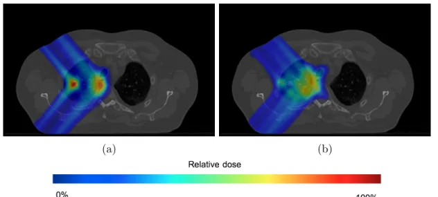
Nous avons ensuite ´evalu´e le calcul de dose sur des cas de patients. Les r´esultats ont montr´e une bonne coh´erence (voir Figure2.4) malgr´e l’apparition d’artefacts syst´emiques dans les diff´erents cas utilis´es. Ces artefacts situ´es sur l’extr´emit´e distale de la tumeur pr´esentent une r´egion de sur-dose (points chauds), le long du contour de la tumeur et une r´egion sous-dos´ee (points froids) apr`es la tumeur (voir Figure 2.5). La cause de cet artefact n’a pas pu ˆetre mise en ´evidence mais pourrait venir de diff´erences dans le calcul de la profondeur radiologique ProtonMachine et MSPT.
(a) (b)
Figure 2.4 – Distribution de dose simul´ee pour un patient dans ProtonMachine (2.4a) et dans MSPT (2.4b).
Points froids
Points chauds
Figure 2.5 – Points chauds et points froids (respectivement situ´es par les rectangles
rouge et bleu).
Nous avons enfin utilis´e le simulateur pour rendre compte de la d´egradation de la dose re¸cue par le patient lors de mouvements intra-fraction (voir Figure2.6). Cette d´egradation se traduit par une irradiation r´eduite de la r´egion de la tumeur, une irradiation accentu´ee
MSPT: Motion Simulator for Proton Therapy
dans les OARs et l’apparition de points chauds et de points froids.
(a) (b)
Figure 2.6 – Distributions de dose calcul´ees pour un patient statique (2.6a) et un patient mobile (2.6b) dans MSPT.
2.4
Compensation du mouvement
Enfin, nous proposons une nouvelle approche de compensation de mouvement bas´ee sur l’adaptation du poids de chaque faisceau en fonction du mouvement et sur la posibilit´e de balayer plusieurs fois un mˆeme position pour une ´energie donn´ee. Le travail effectu´e correspond `a une ´etude pr´eliminaire de cette strat´egie afin de mettre en avant les int´erˆets et les limites.
Consid´erons un plan de traitement pour lequel les positions du faisceau de protons d’´energie En sont repr´esent´ees par les couples (bi, wi) ordonn´es suivant l’indice i. bi
cor-respond aux coordonn´ees de la position du faisceau et wi son poids. Ce plan de traitement
engendre l’irradiation de l’ensemble des (Pi), correspondant aux points cibles des positions
(bi, wi) (la position (bk, wk) irradie le point (Pk) pour un patient statique) du faisceau,
situ´es dans le patient sur la couche d’´energie associ´ee `a En (ensemble des points situ´es
`
a la distance dBP de la source du faisceau, o`u dBP correspond `a la profondeur du pic de
Bragg).On consid`ere que (Pi) est irradi´e par le faisceau (t = i, w = wi) o`u t correspond `a
la date d’irradiation d´efinie par l’ordre des positions du faisceau et w correspond au poids du faisceau. La strat´egie de compensation consiste `a changer w de telle sorte qu’`a t = i, w soit fix´e `a wk afin d’irradier le point (Pk) le point cible du faisceau `a t = i en raison du
mouvement d´efini par le vecteur v(t) situ´e dans le plan perpendiculaire au faisceau. La Figure 2.7 illustre ce principe.
MSPT: Motion Simulator for Proton Therapy
Figure 2.7 – Illustration du traitement, pour un patient mobile, utilisant la technique de compensation. Les positions du faisceau sont repr´esent´ees envert, le faisceau en rouge, les points cibles en bleu et le vecteur de d´eplacement du patient (2D) enorange.
L’´evaluation de cette m´ethode nous a permis de montrer qu’elle r´eduit fortement l’im-pact du mouvement sur la r´epartition de dose dans le patient. Les erreurs de r´epartition de dose obtenues, par rapport `a la r´epartition dans un patient statique, sont tr`es faibles (inf´erieures `a 5%) et le crit`ere indiquant que 95% du volume de la tumeur re¸coit au moins 95% de la dose prescrite est rempli. Par cons´equent, les erreurs peuvent ˆetre consid´er´ees comme cliniquement acceptables. La Figure 2.8 correspond aux courbes repr´esentant le volume relatif de la tumeur et d’OARs, recevant au moins une certaine dose, appel´ees DVHs (Dose Volume Histogram). Ces DVHs sont obtenus pour un patient statique et un patient mobile avec et sans la technique de compensation. Les distributions de dose correspondantes sont repr´esent´ees avec une image CT dans la Figure 2.9. Notre strat´egie permet pour le moment de compenser seulement des mouvements 2D perpendiculaires au faisceau. Un d´eveloppement en 3D pourrait donc faire partie de futurs travaux de recherches et d’am´eliorations. De plus, les mouvements simul´es n’´etant bas´es que sur une transformation rigide du corps du patient, une future ´etude pourrait porter sur la com-pensation des mouvements pr´esent´ee pour des transformations d´eformables.
MSPT: Motion Simulator for Proton Therapy
0
500
1,000 1,500 2,000
0
20
40
60
80
100
95 95% de la dose prescriteDose (cGy)
Relativ
e
V
olume
(%)
Test 1
Test 3
Test 5
Spinal Cord
Right Lung
PTV
Figure 2.8 – Comparaison des DVHs pour un traitement d´elivr´e `a un patient statique (Test 1) et `a un patient mobile avec (Test 5) et sans (Test 3) compensation pour un mouvement de 1.5 cm d’amplitude. Les structures du patient consid´er´ees sont la tumeur (PTV), le poumon droit (Right Lung) et la moelle ´epini`ere (Spinal Cord).
(a)
(b) (c)
Figure 2.9 – Distributions de dose pour un patient statique (2.9a) et un patient mobile sans (2.9b) et avec (2.9c) compensation.
Chapitre 3
Quelques r´
esultats en photon
th´
erapie
3.1
Aspects algorithmiques de la photon th´
erapie
Comme mentionn´e pr´ec´edemment (Section 1.3), en photon th´erapie la planification d’un traitement g´en`ere des plans d’intensit´e correspondant `a des grilles en 2 dimensions. Par cons´equent, chaque grille peut ˆetre repr´esent´ee comme une matrice 2D, appel´ee ma-trice d’intensit´e. Le probl`eme demandant de trouver pour un plan d’intensit´e l’ensemble des configurations permettant de r´ealiser ce plan peut alors ˆetre consid´er´e comme un probl`eme de d´ecomposition de matrice en matrices binaires. Dans ces matrices binaires, les 0 correspondent aux r´egions o`u le MLC bloque le faisceau de photons, et les 1 aux r´egions o`u il irradie le patient. Les probl`emes de minimisation des crit`eres total beam-on time et total setup time peuvent alors correspondre, respectivement, `a des contraintes de minimisation du nombre de matrices binaires et de minimisation de la somme des coeffi-cient des matrices binaires. Ces coefficoeffi-cients sont appel´es poids.
3.2
Pr´
ec´
edents r´
esultats algorithmiques
De pr´ec´edents travaux sur le MLC conventionnel ont montr´e que le probl`eme de mini-misation du total beam-on time peut ˆetre r´esolu en temps lin´eaire [Ahuja and Hamacher,
2005].
Burkard[2002] a prouv´e que le probl`eme de minimisation du total setup time est NP-Difficile pour les matrices d’intensit´e ayant au moins 2 lignes. Ce r´esultat a ´et´e renforc´e par Baatar et al. [2005] qui ont montr´e que ce probl`eme reste NP-Difficile mˆeme pour les matrices `a 1 ligne.
MSPT: Motion Simulator for Proton Therapy
3.3
R´
esultats algorithmiques pour de nouveaux MLCs
Dans le cadre de ce travail nous nous sommes int´eress´es `a deux nouvelles technolo-gies de MLC : le MLC rotatif, dans lequel des rotations de 90◦ sont autoris´ees entre 2 configurations et le MLC double couche, correspondant `a deux couches de paires de lames perpendiculaires entre elles (voir Figure 3.1).
Figure 3.1 – Sch´emas d’un MLC rotatif (gauche) et d’un MLC `a double couche (droite).
Dans une premi`ere partie de l’´etude nous avons d´emontr´e que le probl`eme de d´ecomposition dans le cas d’un MLC `a double couche est NP-Difficile lorsque l’on cherche `a minimiser le crit`ere total setup time. Ensuite, nous avons d´emontr´e que le probl`eme de d´ecomposition dans le cas d’un MLC rotatif est ´egalement NP-Difficile lorsque l’on cherche `a minimiser les crit`eres total setup time et beam on time. De plus, nous proposons un algorithme d’approxi-mation en temps polynomial permettant de fournir une solution enti`ere au probl`eme de d´ecomposition pour un MLC rotatif minimisant le beam on time. Cet algorithme consiste `
a chercher dans un premier temps une solution optimale continue o`u les poids des matrices sont des valeurs r´eelles positives (la contrainte de valeurs enti`eres est relax´ee). Les poids des configurations horizontales sont ensuite arrondis afin d’avoir une solution enti`ere pour ces configurations. La soustraction de cette solution horizontale `a la matrice d’intensit´e initiale correspond `a la matrice d’intensit´e `a d´ecomposer en utilisant des configurations verticales du MLC. Cette d´ecomposition utilisant des valeurs enti`eres est r´ealisable en temps lin´eaire ([Ahuja and Hamacher, 2005]). La solution enti`ere verticale nous permet ainsi d’obtenir une solution enti`ere, pour le probl`eme de d´ecomposition utilisant un MLC rotatif, garantissant une bonne approximation qui est au plus `a 2m de la solution optimale continue o`u m correspond au nombre de paires de lames du MLC.
Chapitre 4
Conclusion
Au cours de cette th`ese, nous nous sommes int´eress´es au domaine de la radiation th´erapie. Nous avons principalement travaill´e au d´eveloppement d’un simulateur de mou-vement pour la proton th´erapie utilisant la technique de balayage. Le but de ce simu-lateur est de fournir un outil permettant de rendre compte de l’impact de mouvements intra-fraction sur le traitement re¸cu par le patient. Un int´erˆet de ce simulateur est de pouvoir comparer des plans de traitement afin de trouver celui qui est le plus robuste `a ces mouvements. De plus, il permet d’´etudier des m´ethodes de r´eduction de l’impact du mouvement comme celle que nous proposons afin d’am´eliorer la qualit´e des traitements et de les rendre moins sensibles aux mouvements intra-fraction. Enfin, nous nous sommes int´eress´es au probl`eme de configurations des MLCs pour de nouvelles technologies bas´ees sur une double couche de MLCs et un MLC rotatif. Nous avons montr´e que trouver une s´equence de configurations, pour ces deux types de MLCs, minimisant le total beam on time et/ou le total setup time est NP-Difficile. Cependant nous proposons un algorithme d’approximation pour r´esoudre le probl`eme de minimisation du total beam on time dans le cas d’un MLC rotatif.
Ces diff´erents travaux nous ont permis d’une part de rendre accessible un logiciel amen´e `
a ´evoluer pour permettre d’autres ´etudes visant `a am´eliorer la qualit´e des traitements de proton th´erapie en cas de mouvements intra-fraction. D’autre part ils ont permis d’´etudier une nouvelle approche pour compenser ces mouvements et ainsi rendre les traitements plus robustes. Enfin, l’´etude du s´equen¸cage de nouveaux types de MLCs nous a permis de mettre en avant aussi bien les probl`emes algorithmiques qu’ils soul`event pour de futures recherches, que l’int´erˆet de leur utilisation.
Foreword
MSPT: Motion Simulator for Proton Therapy
My PhD studies started in September 2011. After working in computer science ap-plied to medical imaging during one year at Casilab (University of North Carolina, Chapel Hill, USA), one year and a half at Imaging Informatics (University of Calgary, Canada) and obtaining a master’s degree from CPE-Lyon (Chimie Physique Electronique, Lyon, France) in computer science, I decided to pursue my studies with a PhD applied to the field of medicine. Indeed, this field is really motivating since computer science can pro-vide advanced tools and information to doctors and to medical personnel to diagnose, treat and cure patients. This is how I came to choose this PhD thesis related to the use of computer science in radiation therapy in the AlgoB team of the LIGM (Laboratoire d’Informatique Gaspard Monge) at the Universit´e Paris-Est Marne La Vall´ee (France).
This PhD thesis falls within the ANR BIRDS 1 (Agence Nationale de la Recherche -BIological networks, RaDiotherapy and Structures) project. This project encompasses 3 distinct tasks. The first and second tasks dedicated to the study of algorithmic in the field of algorithmic structures and in the field of biological networks, which are the main topics of research in the AlgoB team. The third task aims at exploring new areas of research, for the team, where algorithmic and computer science could lead to improvements, and more specifically in radiation therapy. Initially, this third task focused on an algorithmic study of a specific device called Multi-Leaf Collimator (MLC) used in photon therapy, a sub-field of radiation therapy (also known as radiotherapy). With this aim in mind, Dr. Guillaume Blin, in charge of this project, started collaborating with Dr. Xiaodong Wu and the department of Radiation Oncology at the University of Iowa (Iowa, USA) in February 2011. After the beginning of my PhD, thanks to this collaboration we started to realize that the proton therapy, another technique of radiation therapy could offer in-teresting problems that could be addressed with computer science, such as the patient motions during the treatment delivery. Therefore, we broaden the study of radiation ther-apy, not only to photon therther-apy, but also to proton therapy. This collaboration allowed me to build and improve my knowledge in radiation therapy from a physical and a clinical point of view.
1. http://igm.univ-mlv.fr/AlgoB/BIRDS/
Contents
Table of Contents
Acknowledgments
ii
Abstract / R´
esum´
e
iv
R´
esum´
e de la th`
ese en Fran¸
cais
vi
1 Radiation th´erapie vii
1.1 Pr´esentation de la radiation th´erapie . . . vii
1.2 Comparaison entre la photon et la proton th´erapie . . . viii
1.3 Des challenges en radiation th´erapie . . . ix
2 MSPT : Un simulateur de mouvement pour la proton th´erapie xii
2.1 D´eveloppement d’un outil pour l’´etude des mouvements intra-fraction.. . . xii
2.2 Mod´elisation. . . xiii
2.3 Evaluation du simulateur . . . xiv
2.4 Compensation du mouvement . . . xvi
3 Quelques r´esultats en photon th´erapie xix
3.1 Aspects algorithmiques de la photon th´erapie . . . xix
3.2 Pr´ec´edents r´esultats algorithmiques . . . xix
3.3 R´esultats algorithmiques pour de nouveaux MLCs . . . xx
4 Conclusion xxi
Foreword
xxiv
Contents
xxvi
Table of Contents xxix
List of Tables xxxi
List of Figures xxxv
MSPT: Motion Simulator for Proton Therapy Glossary xxxvi Glossary . . . xxxvi Acronyms . . . xxxviii
Introduction
2
I
Radiation Therapy
4
1 History of the radiation therapy 5
2 Principles and physics of radiation therapy techniques 9
2.1 External beam radiation therapy . . . 9
2.1.1 Principle . . . 9
2.1.2 Particle accelerators . . . 10
2.2 Internal beam radiation therapy . . . 13
2.3 Protons and photons in radiation therapy. . . 14
2.3.1 Establishment and cost comparison . . . 14
2.3.2 Radiation comparison . . . 14
2.4 Process of a radiation therapy treatment . . . 15
2.4.1 General treatment planning . . . 15
2.4.2 Photon therapy planning and delivery . . . 16
2.4.3 Proton therapy planning and delivery . . . 18
2.5 Radiation therapy challenges . . . 21
2.5.1 Uncertainties in radiation therapy . . . 21
2.5.2 Mitigation techniques in radiation therapy . . . 21
2.5.3 Intra-fraction motion in proton therapy . . . 22
II
MSPT: Motion Simulator for Proton Therapy
24
1 MSPT a new tool to study intra-fraction motions 25
1.1 Development of a proton therapy motion simulator . . . 25
1.2 MSPT objectives . . . 26
1.2.1 Render the impact on the dose distribution . . . 26
1.2.2 Improve the treatment robustness . . . 26
2 Simulator implementation 27
2.1 Simulator implementation . . . 27
2.2 About MSTP’s development . . . 27
2.3 The DICOM standard . . . 28
2.4 Simulator inputs and outputs . . . 31
2.5 Simulator architecture . . . 32
MSPT: Motion Simulator for Proton Therapy
3 Physics models 37
3.1 Coordinate systems . . . 37
3.2 Patient and motion models . . . 40
3.2.1 Patient representation . . . 40 3.2.2 Motion management . . . 41 3.3 Dose calculation . . . 45 3.4 Delivery process . . . 48 4 Simulator evaluation 50 4.1 Simulations in water . . . 50
4.2 Simulations on patient datasets . . . 53
4.2.1 Example of patient case simulation . . . 54
4.2.2 Artifact observed in the dose distribution . . . 56
4.2.3 Overall comparison . . . 58
4.3 Impact of motion . . . 63
5 Compensation technique 67
5.1 Principle of the compensation technique . . . 68
5.2 Strategy of the compensation technique . . . 70
5.2.1 Strategy presentation . . . 70
5.2.2 Compensation algorithm . . . 72
5.3 Evaluation of the compensation . . . 73
5.3.1 Evaluation of the compensation for moderate amplitude motions . . 75
5.3.2 Evaluation of the compensation for large amplitude motions . . . . 78
5.3.3 Compensation with and without margin . . . 81
5.3.4 Evaluate the impact of the monitoring system accuracy . . . 83
5.4 Discussion on the compensation . . . 86
Closing remarks on MSPT 88
MSPT’s advantages. . . 88
MSPT’s limitations . . . 88
III
Some Results in Photon Therapy
89
1 Algorithmic aspects of photon therapy 90
2 Algorithmic results in photon therapy 92
2.1 Previous algorithmic results . . . 92
2.2 Technological variants of MLCs . . . 96
2.2.1 Rotating MLC . . . 96
2.2.2 Multi-Layer MLC . . . 97
2.3 Algorithmic results for new MLC variants . . . 98
2.3.1 Algorithmic results for Dual MLC . . . 98
2.3.2 Algorithmic results for Rotating MLC . . . 100
MSPT: Motion Simulator for Proton Therapy
Conclusion and future directions
110
Conclusion 110
Future work 112
Bibliography 112
List of Tables
2.1 Portion of a CT Image object representing a 2D slice of the patient CT image. . . 29
2.2 Portion of a RT Structure Set object storing the contours of the regions of interest in the patient. . . 29
2.3 Portion of a RT Plan object storing the entire treatment plan. . . 30
2.4 Portion of a RT Dose object storing the 3D dose distribution. . . 31
3.1 Temporal values of some delivery’s events. . . 49
4.1 Patient cases summary . . . 54
4.2 Dose received by 95% and 5% of the tumor volume for simulations in Pro-tonMachine and in MSPT. . . 55
4.3 Volume receiving 10, 33, 50, 66 and 90 % of the prescribed dose and the average dose received by the OARs in ProtonMachine and in MSPT. . . 55
4.4 Average error of the dosimetric parameters in the tumor volumes of the different patient cases. The error is relative to the maximum dose of the tumor volume. . . 61
4.5 Average error of the dosimetric parameters in the OARs of the different patient cases. . . 62
4.6 Dose received by 95% and 50% of the tumor volume for the delivery of a treatment plan simulated, for a patient static and the same patient moving, in MSPT. . . 64
5.1 Table summarizing the tests performed to evaluate the compensation method. 74
5.2 Dose received by 95% and 5% of the PTV on a static and dynamic patient with and without compensation for a 0.5 cm motion amplitude. . . 77
5.3 Volume receiving 10, 33, 50, 66 and 90 % of the prescribed dose and the average dose received by the OARs in MSPT on a static and dynamic patient with and without compensation for a 0.5 cm motion amplitude. . . 77
5.4 Dose received by 95% and 5% of the PTV on a static and dynamic patient with and without compensation for a 1.5 cm motion amplitude. . . 80
5.5 Volume receiving 10, 33, 50, 66 and 90 % of the prescribed dose and the average dose received by the OARs in MSPT on a static and dynamic patient with and without compensation for a 1.5 cm motion amplitude. . . 80
MSPT: Motion Simulator for Proton Therapy
5.6 Dose received by 95% and 5% of the PTV on a dynamic patient for a delivery using the compensation strategy with and without margin for a 1.5 cm motion amplitude. . . 82
5.7 Volume receiving 10, 33, 50, 66 and 90 % of the prescribed dose and the average dose received by the OARs in MSPT on a dynamic patient for a delivery using the compensation strategy with and without margin for a 1.5 cm motion amplitude. . . 82
5.8 Re-scanning statistics for a delivery using compensation with and without margin. . . 83
5.9 Dose received by 95% and 5% of the PTV on a dynamic patient for a de-livery using the compensation strategy for different accuracy of the motion monitoring system. . . 85
5.10 Volume receiving 10, 33, 50, 66 and 90 % of the prescribed dose and the average dose received by the OARs in MSPT on a dynamic patient with compensation for different accuracy of the motion monitoring system. . . . 85
5.11 Table summarizing the average dosimetric differences, for the tumor, for different values of σδ, and where the delivery with σδ = 0 cm is considered
as the benchmark. . . 86
5.12 Table summarizing the average dosimetric differences, for the OARs, for different values of σδ, and where the delivery with σδ = 0 mm is considered
as the benchmark. . . 86
List of Figures
1.1 Radiation th´erapie externe. . . vii
1.2 Profils de dose pour des photons et des protons. . . viii
1.3 Comparaison de la dose d´epos´ee dans un patient pour des photons et des protons. . . ix
1.4 Exemples de MLCs.. . . x
1.5 Illustration de la technique de balayage. . . xi
1.6 R´esultat de l’irradiation d’une plaque radiographique avec et sans mouve-ments. . . xi
2.1 Exemple d’une image CT et de la repr´esentation de diff´erentes structures du patient : poumons, r´egion cible comprenant la tumeur, moelle ´epini`ere et des os de la colonne vert´ebrale. . . xiii
2.2 Exemple d’une image CT et de la repr´esentation de la r´epartition de dose simul´ee dans MSPT. . . xiii
2.3 Graphiques repr´esentant la dose en fonction de la profondeur et le profil lat´eral de la r´epartition de dose d’un faisceau de protons de 210MeV dans l’eau avec ProtonMachine et MSPT. . . xiv
2.4 Distribution de dose simul´ee pour un patient dans ProtonMachine et dans MSPT. . . xv
2.5 Points chauds et points froids. . . xv
2.6 Distributions de dose calcul´ees pour un patient statique et un patient mo-bile dans MSPT. . . xvi
2.7 Illustration du traitement, pour un patient mobile, utilisant la technique de compensation. . . xvii
2.8 Comparaison des DVHs pour un traitement d´elivr´e `a un patient statique et `a un patient mobile avec et sans compensation pour un mouvement de 1.5 cm d’amplitude. Les structures du patient consid´er´ees sont la tumeur,
le poumon droit et la moelle ´epini`ere. . . xviii
2.9 Distributions de dose pour un patient statique et un patient mobile sans
et avec compensation. . . xviii
3.1 Sch´emas d’un MLC rotatif et d’un MLC `a double couche. . . xx
1.1 Dr. Roentgen’s first X-ray image. . . 5
1.2 1954: First treated patient at the Lawrence Berkeley Laboratory. . . 7
2.1 Schematic of an external beam radiation therapy system . . . 9
MSPT: Motion Simulator for Proton Therapy
2.2 Example of a linac in a photon therapy gantry.. . . 10
2.3 Schematic of a cyclotron. . . 11
2.4 Schematic of a synchrotron. . . 12
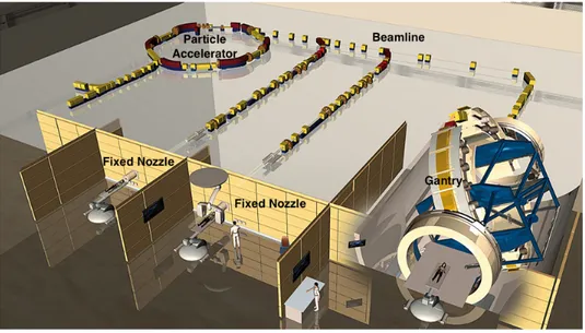
2.5 Schematic of a proton therapy center. . . 12
2.6 Gantry in a proton therapy treatment room. . . 13
2.7 Schematic of the brachytherapy principle.. . . 13
2.8 Dose profiles for photons and protons. . . 14
2.9 Comparison of deposited dose for a treatment: photons versus protons. . . 15
2.10 IMRT grantry angles and some intensity maps. . . 17
2.11 Examples of MLCs. . . 17
2.12 Principle of energy layers . . . 19
2.13 Scheme of beam scattering delivery . . . 19
2.14 Example of brass aperture and range compensator . . . 20
2.15 Scheme of the spot scanning technique. . . 20
2.16 Results of irradiation without and with motion on a radiographic film.. . . 22
2.1 Example of visual outputs: a CT slice with several binary masks of different body structures and the dose distribution of a single proton pencil beam. . 32
2.2 Class diagram of MSPT. . . 32
2.3 Diagram representing the dependencies used to build a Patient. . . 35
2.4 Diagram representing the main function calls from the Patient object to initialize and update the patient model. . . 35
2.5 Diagram representing the relationships between the classes used to simulate the delivery of a treatment in SimulatorDelivery). . . 36
2.6 Diagram representing the main function calls from the SimulatorDelivery object during the simulation of a delivery. . . 36
3.1 DICOM patient coordinate system and voxel indexing system. . . 38
3.2 IEC Coordinate systems . . . 39
3.3 Conversion from CT# to mass density . . . 40
3.4 Illustration of x(t) for the ideal breathing motion model: bx = 1.5 cm,
τx = 4.0 s, φx= 0 rad. . . 41
3.5 Illustration of x(t) for the irregular breathing model: bx = 1.5 cm, σbx = 0.15 cm, τx = 4.0 s, στx = 0.4 s, φx = 0 rad. . . 43 3.6 Illustration of x(t) with the hiccup model: bx = 1.5 cm, σbx = 0.15 cm,
τx = 4.0 s, στx = 0.4 s, φx = 0 rad.. . . 44 3.7 Illustration of x(t) with the cough model: bx = 1.5 cm, σbx = 0.15 cm,
τx = 4.0 s, στx = 0.4 s, φx = 0 rad.. . . 44 3.8 Dose correction factor λ as a function of energy. . . 46
3.9 Stopping power correction factor as a function of mass density. . . 47
4.1 Plot representing the depth dose curve for the beamlet dose distributions obtained at 55 MeV, 130 MeV and 210 MeV with ProtonMachine and MSPT in water, for the same monitor units. . . 51
MSPT: Motion Simulator for Proton Therapy
4.2 Absolute difference of Bragg Peak depth for beamlets simulated with Pro-tonMachine and MSPT for energies ranging from 30 MeV to 230 MeV in water. . . 51
4.3 Plot representing the lateral profiles at the Bragg Peak for the beamlet dose distributions obtained at 55, 130 and 210 MeV with ProtonMachine and MSPT in water. . . 52
4.4 Plot representing sigma for the dose distributions computed in ProtonMa-chine and MSPT for energies ranging from 30 MeV to 230 MeV in water. . . 53
4.5 DVH comparison between ProtonMachine and MSPT for the lung tumor case. 55
4.6 Dose distributions computed in ProtonMachine and in MSPT overlaying the patient CT image. . . 56
4.7 Dose distributions computed in ProtonMachine and in MSPT overlaying the patient CT image. . . 57
4.8 DVH comparison between ProtonMachine and MSPT: observation of hot spots in the PTV and cold spots after the tumor (right lung) in MSPT dose distribution. . . 57
4.9 Hot and cold spots present in the comparison of the dose distributions (Figure 4.7). . . 58
4.10 DVHs of the 8 patient cases for ProtonMachine and MSPT . . . 59
4.11 Images of the dose distributions of patient cases HN1, Lung1, Lung2 and Lung3 for ProtonMachine and MSPT . . . 60
4.12 Images of the dose distributions of patient cases Lung4, Lung5, Lung6 and Pelvis1 for ProtonMachine and MSPT . . . 61
4.13 Comparison of DVHs for a delivery on a static and dynamic patient.. . . . 64
4.14 Dose distributions computed overlaying a patient CT image (transverse planes), for a static and a moving patient. . . 65
4.15 Hot and cold spots present in the dose distribution of the moving patient overlaying the patient CT image (transverse planes). . . 65
5.1 Illustration of the beam gating delivery. . . 67
5.2 Illustration of the beam tracking system. . . 68
5.3 Illustration of the delivery for a static patient. . . 69
5.4 Illustration of the delivery for a moving patient without the compensation technique. . . 69
5.5 Illustration of the delivery for a moving patient with the compensation technique. . . 70
5.6 Illustration of the delivery for a moving patient with the compensation technique where a margin is added around the planned positions. . . 71
5.7 Example of a 2D representation of the beam positions, the margin region and the region where no beam position is defined for a single energy layer. 72
5.8 Delineation of the tumor and the OARs overlaying a patient CT image (transverse and coronal plane) . . . 74
5.9 Dose distributions computed overlaying a patient CT image (transverse planes), for a static and a moving patient without and with compensation. 75
5.10 Dose distributions computed overlaying a patient CT image (coronal planes), for a static and a moving patient without and with compensation. . . 76
MSPT: Motion Simulator for Proton Therapy
5.11 Comparison of DVHs for a delivery on a static and dynamic patient with and without compensation for a 0.5 cm motion amplitude. . . 76
5.12 Dose distributions computed overlaying a patient CT image (transverse planes), for a static and a moving patient without and with compensation. 78
5.13 Dose distributions computed overlaying a patient CT image (coronal planes), for a static and a moving patient without and with compensation. . . 79
5.14 Comparison of DVHs for a delivery on a static and dynamic patient with and without compensation for a 1.5 cm motion amplitude. . . 79
5.15 Dose distributions computed overlaying a patient CT image (transverse planes), for a moving patient using the compensation strategy with and without margin. . . 81
5.16 Dose distributions computed overlaying a patient CT image (coronal planes), for a moving patient using the compensation strategy with and without margin. . . 81
5.17 Comparison of DVHs for a compensated delivery on a dynamic patient for a 1.5 cm motion amplitude with and without margin. . . 82
5.18 Dose distributions computed overlaying a patient CT image (transverse planes), for a moving patient with compensation for different monitoring accuracy: σδ= 0 cm, 0.3 cm, 0.75 cm, 1.5 cm. . . 84
5.19 Dose distributions computed overlaying a patient CT image (coronal planes), for a moving patient with compensation for different monitoring accuracy: σδ = 0 cm, 0.3 cm, 0.75 cm, 1.5 cm. . . 84
5.20 Comparison of DVHs for a delivery on a dynamic patient with compensa-tion for a 1.5 cm mocompensa-tion amplitude to evaluate the impact of the mocompensa-tion monitoring system accuracy. . . 85
2.1 Schematic of a rotating MLC . . . 97
2.2 Schematic of a dual-MLC . . . 98
2.3 Illustration of Matrix M . . . 100
2.4 Integer Linear Program minimizing the total beam-on time for MOD . . . 104
2.5 Rounding technique initial state . . . 105
2.6 Rounding technique: first step . . . 106
2.7 Rounding technique: second step - 1 . . . 106
2.8 Rounding technique: second step - 2.1 . . . 106
2.9 Rounding technique: second step - 2.2 . . . 107
2.10 Rounding technique: Set of stacks . . . 107
2.11 Rounding technique: Rounded solution . . . 108
Glossary
Glossary
CT Number
CT Number is a value assigned to a voxel in a CT image. This value is based on the Hounsfield Unit. CT numbers for air, water and compact bone are respectively -1000HU, 0HU, and +1000HU.
Gray
Unit representing the absorbed dose by a medium for ionizing radiation. One gray is the absorption of one joule of energy, per kilogram of matter:
1Gy = 1kgJ.
Hounsfield Unit
Unit to scale the linear attenuation coefficient of a medium compared to the linear attenuation coefficient of water:
HU = 1000 × µX−µW ater
µW ater , where µX is the linear attenuation coefficient (m
−1) of
the medium X, depending on the atomic number, the mass density and the photon energy.
Mega-electron Volt
1 MeV is equal to 1.60217657 × 10⁻¹³ Joules. It corresponds to the energy gained or lost by the charge of 106 electrons moving across an electric potential difference
of 1 Volt.
Stereotactic Body Radiation Therapy
Stereotactic Body Radiation Therapy is a treatment procedure involving high dose fractions.
Computed Tomography
Computed tomography is an anatomical imaging technique using X-rays (photons) that allows the acquisition of a 3D image of a patient. It provides especially a good rendering of dense tissues such as bones.
Dose-Volume Histogram
A dose-volume histogram is a 2D plot representing the percentage of volume receiv-ing a certain amount of dose.
Magnetic Resonance Imaging
Magnetic Resonance Imaging is an anatomical imaging technique using variable magnetic fields that allows the acquisition of a 3D image of a patient. It provides especially a good rendering of soft tissues such as ligaments.
MSPT: Motion Simulator for Proton Therapy
Positron Emission Tomography
Positron Emission Tomography is a functional imaging technique using the detec-tion of pairs of gamma-rays produced indirectly by a positron-emitting radioisotope injected in the patient bloodstream. This technique allows a 3D acquisition of the biological activity of a patient.
Single Photon Emission Computed Tomography
Single Photon Emission Computed Tomography is a functional imaging technique using gamma rays obtained by injecting a radioisotope in the patient bloodstream. This technique allows a 3D acquisition of the biological activity of a patient.
Treatment Planning System
Software used to plan and optimize a treatment plan. Radiological Depth
The radiological depth at point P in a medium is the thickness of water having the same effect on the particle energy as the thickness from the beam’s entrance into the medium to a given point P .
Let’s consider a beam of energy E1 entering into a patient body. At point P located at
a depth DM, the beam’s energy drops to E0. In water, a beam entering with the energy
E1, will loose some energy and reach E0 at depth DW. Hence, the radiological depth at
P is DW.
Voxel
Volume element representing the resolution of a 3D matrix.
MSPT: Motion Simulator for Proton Therapy
Acronyms
2D 2-dimensions. 3D 3-dimensions. 4D 4-dimensions.
CFRT Conformal Radiation Therapy.
CT Computed Tomography.
CT# CT Number.
CTV Clinical Target Volume.
DICOM Digital Imaging and Communications in Medicine.
DVH Dose Volume Histogram.
GTV Gross Tumor Volume.
Gy Gray.
HU Hounsfield Unit.
IEC International Electrotechnical Commission. IMRT Intensity Modulated Radiation Therapy.
linac Linear Accelerator.
MeV Mega-electron Volt.
MLC Multileaf Collimator.
MRI Magnetic Resonance Imaging.
MU Monitor Units.
OAR Organ At Risk.
PET Positron Emission Tomography. PRV Planning organ at Risk Volume. PTV Planning Target Volume.
SBRT Stereotactic Body Radiation Therapy.
SPECT Single Photon Emission Computed Tomogra-phy.
TPS Treatment Planning System.
Introduction
MSPT: Motion Simulator for Proton Therapy
Radiation therapy is one of the most common cancer treatments. It uses ionizing radiation to kill cells within a tumor. A treatment aims at irradiating with high dose the tumor and at protecting the so-called organs at risk (OARs), which correspond to healthy tissues sensitive to radiation. A treatment can be delivered using different types of radiation: photon-based radiation in the so-called photon therapy, and proton-based radiation in the so-called proton therapy. Photon therapy is much more used than proton therapy. Indeed, as of August 2013, the number of proton therapy centers represents 1% of the photon therapy centers [Goethals and Zimmermann, 2013]. The main reason for this difference is the cost of such medical centers. However, proton therapy arouses more and more interests due to its advantages in providing an accurate irradiation of the tumor combined with a good sparing of healthy tissues and organs at risk. It was shown that protons are preferable to photons, in particular, when it comes to treat tumors close to dose-sensitive anatomical structures such as in head-and-neck treatments [Chan and Liebsch, 2008], prostate cancer [Lee et al., 1994] or when it is essential to reduce toxicity to healthy tissues such as in pediatric patients [Fuss et al., 1999], [Clair et al.,
2004]. Moreover, it was shown that protons allow a greater tumor control probability and a smaller normal tissue complications probability than photons [Fuss et al., 1999], [Fuss et al., 2000], [Lin et al., 2000]. This is one of the reasons why more and more studies focus on this type of radiation therapy both on the clinical and the physical sides.
In proton therapy, mainly two techniques can be used: the scattering and the spot scanning. However, we focused on the spot scanning delivery strategy. It consists of a thin proton beam scanned across the tumor volume. It provides a good conformity to complex tumor shapes, which reduces toxicity to healthy tissues. However, this accuracy is greatly degraded when the patient moves during the treatment, which is unavoidable since the patient is alive and the lungs and other organs (e.g., the heart) are constantly in motion. Such motions are called intra-fraction motions. The problem of intra-fraction motion has some impact on the overall treatment. The improvement of the treatment’s ro-bustness to motion requires the capacity of dose computation on dynamic patient dataset (i.e., a 4-dimensions (4D) treatment planning). Studies are often conducted with the researcher’s in-house treatment planning system or an expensive clinical treatment plan-ning system. The limited availability of 4D treatment planning system makes it difficult to study this subject by a broader category of researchers. This is why we developed an open-source 4D dose computation and evaluation software, MSPT (Motion Simulator for Proton Therapy). The main interest of this simulator lies in the ability to render the impact of a predicted patient motion on a prescribed treatment plan. This capa-bility makes it an innovative research tool to evaluate and compare different methods of motion management or mitigation. While the main objective of MSPT is to quantify the treatment degradation induced by particular motions, it can also be used to elaborate some compensation methods to improve treatment robustness such as the one we propose.
On the fringe of this work, we tackled algorithmic problems encountered in photon therapy. We focused on the so-called Intensity Modulated Radiation Therapy (IMRT) de-livery technique using MLC. A central problem of this technique requires finding a series of leaves configurations that can be shaped withMLC. From an algorithmic point of view,
MSPT: Motion Simulator for Proton Therapy
this can be considered as a matrix decomposition problem. We analyzed this problem for dual-layer MLCs and rotating MLCs. We propose theoretical results for both types of
MLCs and an approximation algorithm for rotating MLCs.
In the first part of this dissertation, we will introduce the field of radiation therapy and more specifically the proton therapy and photon therapy from an historical and a physical point of view. We will also introduce the problems addressed in the rest of this manuscript: intra-fraction motion in proton therapy and MLC decomposition in photon therapy. In a second part, we will present our simulator MSPT, developped to study the intra-fraction motion and improve the robustness of treatments as regards to motion. We will also propose a new approach to reduce the impact of intra-fraction motions. Finally, we will present algorithmic results and an approximation algorithm for the MLC
decomposition problem.
Part I
Radiation Therapy
Chapter 1
History of the radiation therapy
The history of radiation therapy begins with the discovery of X-rays (photons with an energy level approximately between 60 and 100 KeV) in 1895 by Dr. Wilhelm Roentgen [R¨ontgen, 1896] in Germany. This breakthrough changed the medical world by providing a new non-invasive diagnostic method allowing to see inside a patient in 2-dimensions (2D), thereby giving birth to a new medical specialty: namely, Radiology. Figure 1.1
shows the first radiography obtained by Dr. Roentgen.
Figure 1.1 – Dr. Roentgen’s first X-ray image. The subject was his wife’s hand. [ Baum-rind,2011]
Soon after, it was observed that exposure to X-rays could damage body tissues and in 1896 a first attempt to treat a breast tumor was performed by Dr. Emil H. Grubbe in Chicago (USA) [Science,1957;Vujosevic and Bokorov,2010] using an X-ray machine. It was followed by other attempts such as in 1896 for a stomach cancer by Victor Despeignes in Lyon (France). This was the beginning of a new medical field called radiation oncology [Connell and Hellman,2009] and more specifically external beam radiation therapy.
MSPT: Motion Simulator for Proton Therapy
In 1903, Dr. Henri Becquerel, along with Pierre and Marie Curie, won a Nobel Prize in Physics for the discovery of radioactivity. This team was able to isolate the first known ra-dioactive elements, named Polonium and Radium, that naturally emit ionizing radiation. Their research resulted in a new radiation treatment called brachytherapy (also known as curietherapy or internal radiation therapy). The treatment, which consists in implanting radioactive seeds within a patient was first used in 1901 by Dr. Henri-Alexandre Danlos in Paris (France) [Gupta,1995].
In the 1920’s-30’s the idea of fractionated radiation therapy was introduced. The treatment was divided over the time, instead of a single large exposure, in order to reduce toxicity to healthy tissues in the patient. Nowadays, fractionation is still widely used for all types of radiation therapy techniques [Paganetti et al., 2012].
Early in the development of the radiation therapy, it was recognized that the use of high energy photon beams (greater than a few hundred keV) would provide better out-comes. This technique became known as photon therapy. Initially the equipment could not provide such beams, but in 1924 Gustav Ising invented the particleLinear Accelerator (linac)concept [Ising,1924] which was later used by Rolf Wider¨oe to build alinacin 1928 [Wider¨oe, 1928]. In 1929, Ernest O. Lawrence designed the cyclotron, a ”coiled” linac, inspired by Ising and Wider¨oe research [Bryant, 2010]. As a result of these inventions, high energy photon beams could be generated, from high energy - for that time - electron beams, but also high energy protons and ion beams (e.g., 1.25Mega-electron Volt (MeV)
protons by Lawrence’s cyclotron in 1932 [Bryant,2010]). In 1943, Oliphant proposed the synchrotron concept [Wilson, 1996] to accelerate charged particles. In 1946, Goward and Barnes made a first demonstration of an 8MeV synchrotron at Woolwich Arsenal (UK). Two months later, Elder, Gurewitsch, Langmuir and Pollock, built a 70MeV synchrotron at the General Electric Laboratory in Schenectady (USA).
In 1946, Robert R. Wilson outlined the importance of protons in radiation therapy [Wilson, 1946] explaining that protons of 125MeV could penetrate body tissues up to a range of 12cm and 27cm for protons of 200MeV. In addition, he demonstrated that the bi-ological damage depends on the density of ionization and that, in the case of protons, this density of ionization increases considerably near the end of the range. In 1954, Ernest O. Lawrence used proton beams to treat a first patient at the Lawrence Berkeley Laboratory in California (USA) [Lawrence, 1957; Paganetti et al., 2012]. This was the beginning of proton therapy, another external beam radiation therapy method. Figure 1.2 shows this first patient with Dr. Lawrence.