HAL Id: dumas-01355265
https://dumas.ccsd.cnrs.fr/dumas-01355265
Submitted on 22 Aug 2016
HAL is a multi-disciplinary open access
archive for the deposit and dissemination of sci-entific research documents, whether they are pub-lished or not. The documents may come from teaching and research institutions in France or abroad, or from public or private research centers.
L’archive ouverte pluridisciplinaire HAL, est destinée au dépôt et à la diffusion de documents scientifiques de niveau recherche, publiés ou non, émanant des établissements d’enseignement et de recherche français ou étrangers, des laboratoires publics ou privés.
The growth effect of disaggregated foreign aid : evidence
from bilateral loans and grants
Danny Kurban
To cite this version:
Danny Kurban. The growth effect of disaggregated foreign aid : evidence from bilateral loans and grants. Economics and Finance. 2015. �dumas-01355265�
The Growth Effect of Disaggregated Foreign Aid:
Evidence from Bilateral Loans and Grants
Danny Kurban
Université Paris 1 Panthéon-Sorbonne
UFR 02 – Sciences Économiques
Master 2 Recherche Économie de la Mondialisation
Supervisor: Lisa Chauvet
2
L'université de Paris 1 Panthéon-Sorbonne n'entend donner aucune approbation ni
désapprobation aux opinions émises dans ce mémoire: elles doivent être
considérées comme propre à leur auteur.
The University of Paris 1 Panthéon-Sorbonne neither approves nor disapproves of
the opinions expressed in this dissertation: they should be considered as the
3
Contents
1. Introduction ... 4
2.1 On the heterogeneous effect of foreign aid on growth ... 6
2.2 Grants versus loans ... 8
2.2.1 Asymmetric information and moral hazard: The case for loans ... 9
2.2.2 Debt crises and defensive lending: The case for grants ... 10
2.2.3 Grants versus loans: Does it matter at all? ... 11
3. Data and descriptive statistics ... 11
4. Empirical strategy: How to overcome the endogeneity bias? ... 15
4.1 The problem ... 15
4.2 The different strategies to solve the endogeneity issue ... 17
4.2.1 Lags and differences: Clemens et al. (2012)... 17
4.2.2 Demand-side instruments: Burnside and Dollar (2000) ... 18
4.2.3 Supply-side instruments: Rajan and Subramanian (2008) ... 19
4.2.4 Quasi-experiments : Galiani et al. (2014) ... 21
5. Results ... 23
5.1 Random effects ... 23
5.2 First-difference estimator ... 27
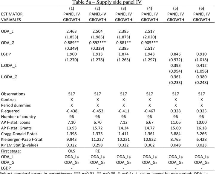
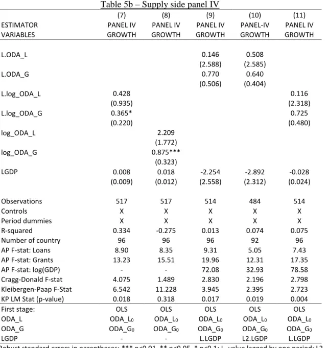
5.3 Supply-side instrumentation strategy ... 31
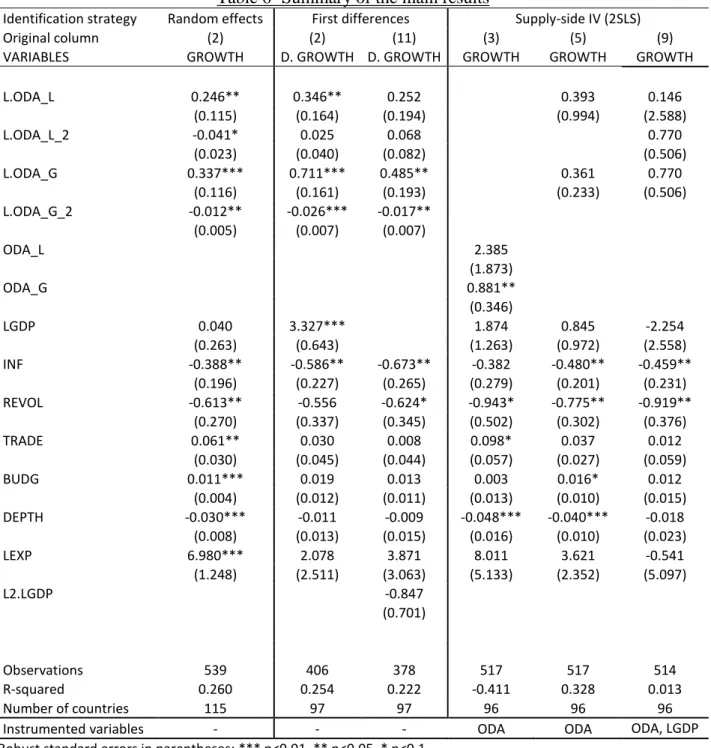
5.4 Summary of the main results ... 36
6. Robustness tests ... 39
7. Conclusion ... 46
References ... 48
4
1. Introduction
The share devoted to foreign aid in developed countries’ government budgets is usually small. But on the side of the recipient country, aid inflows can be rather large, as a share of government revenues and also relative to GDP. Foreign aid thus provides the opportunity for donors to obtain a large positive impact on living conditions in developing countries with relatively little financial effort. However, whether aid really has a positive and measurable effect on economic growth and other development indicators has been intensely debated by economists, with no scientific consensus reached so far. Arndt, Jones, and Tarp (2014) claim that in the long run aid has increased growth, as well as life expectancy and the average years of schooling, while decreasing poverty and infant mortality. Doucouliagos and Paldam (2011) on the other hand show in a meta-study of 105 aid-growth studies that on average, and if the publication bias is controlled for, no significant effect of foreign aid on economic growth has been found in the literature. They further suggest to shift the focus away from aggregate aid measures to more disaggregated ones, which is one of the main motivations for this study. More specifically, the present study disaggregates total aid flows into its grant and loan components and asks if at the least one of them has a significant impact on growth. If both are significant, the question becomes whether their effects are significantly different from each other.
Much like in the case of aid effectiveness in general, the question whether to give foreign aid as non-repayable grants or as repayable loans has been the issue of an intense debate. However, unlike in the aid-growth debate, the discussion has been driven by political rather than economic arguments. From the donor perspective, the decision whether to give aid as grants or loans is probably more motivated by political considerations rather than by their relative efficiency (Sanford (2002), Nunnenkamp, Thiele, and Wilfer (2005)). Nevertheless, there is a strand of literature that assesses the different economic implications of grants and loans with respect to different outcomes, which may be substantial. But again, contrary to the general aid and growth debate, this literature has remained largely theoretical. Empirical results on the differential effects of loan and grant aid in the receiving countries are scarce, perhaps due to the various pitfalls and difficulties that arise if one aims to identify them. Identifying a causal effect of aggregated aid on growth is already challenging, due to the widely recognized problem of endogeneity bias. This has resulted in a large array of studies developing methods to overcome
5
this bias. But if the goal is to empirically identify the impact of disaggregated aid, that is grants and loans, separately, the econometric challenges become even greater, due to the additional problem of multicollinearity and joint determination. Nevertheless, the theoretical arguments for different effects of loans and grants seem strong enough to warrant a comprehensive empirical investigation, despite the obvious difficulties lying ahead.
Hence, the research question addressed in this paper asks about the differential effect of two highly correlated and most likely endogenous factors on growth. Even though there are reasons to believe that the true effects of grants and loans differ, as the next section will show, this difference may be so small that it is practically impossible to detect and economically insignificant. However, the failure to detect any significant differential effect in the empirical estimation does not mean that it is too small to be detected or even non-existent. It could also be due to the problems of multicollinearity and weak instrumentation, especially in the case of multiple endogenous regressors. If one endogenous regressor gets insignificant when instrumented, it becomes practically impossible to identify whether it is significantly different from other regressors, because confidence bands usually overlap. Thus, in light of these problems, a second contribution of this study, in addition to trying to answer the research question about the growth effects of grants and loans in a satisfactory way, is of a more methodological nature. Using the example of aid-growth regressions with multiple endogenous regressors, the problems of weak instrumentation and multicollinearity as well as the most effective and feasible ways to detect and address them will be discussed. This is especially the case for Sections 4 and 5, which aim at analyzing these problems in an applied manner.
Section 2 gives an overview of the general debate about the effects of aid on growth and the related literature, followed by a summary of the theoretical considerations in favor of loans and grants, respectively. Section 3 introduces the data and shows a few key summary statistics. In Section 4, a detailed explanation of the endogeneity problem in the aid literature and its consequences for empirical studies is given. Afterwards, four of the main identification strategies developed to deal with this problem are analyzed, with a special focus on their feasibility in the context of the specific research question addressed in this paper. Section 5 applies modified versions of two of these strategies and tries to identify an effect of aid, disaggregated to grants and loans, on growth. Section 6 shows the results of an extensive set of robustness tests that have
6
been run in order to address some major threats to the validity of the results, and Section 7 concludes.
2. Theory and literature
This chapter briefly discusses how foreign aid can affect GDP growth from a theoretical point of view and then gives an overview of the previous empirical studies and their most important results (Section 2.1). Due to the vast amount of literature on the topic, this overview remains selective in the choice of works and rather short in their treatment. However, some of the most influential methodological papers will be discussed in greater detail in Section 4. Section 2.2 then reviews the theoretical and empirical contributions that have already been made with regard to the specific research question addressed in this paper: “Is there a difference in the effectiveness of grant aid and loan aid?”
2.1 On the heterogeneous effect of foreign aid on growth
In a standard neoclassical growth model, capital accumulation (i.e. investment) is an important determinant of GDP growth. However, especially for less developed countries, investment is constrained by the difficult access to external sources of financing, as these countries face particularly high borrowing costs on international capital markets. This borrowing constraint can lead to savings and investment rates which are too low from an intertemporal point of view, holding the growth rate below its optimal level. Foreign aid, whether it comes as a permanent transfer (grant) or as a temporal one (concessional loans), can relax the borrowing constraint and thus promote growth. However, in the long run this will only happen when at least part of the aid transfer is used for productive investment, as opposed to unproductive investment or consumption. It is also important that aid is not highly fungible, meaning that it does not just crowd out domestically financed investments and in the process lead to reallocation of resources to other, less productive government activities. Only if aid finances productive investments and if fungibility is low will it help to bring a country closer to its optimal steady state long-run growth rate. In other words, the effect of foreign aid on growth is of course conditional on its use, which in turn can depend on many factors, such as the specific type of aid (technical assistance, grants, loans etc.) or the policy environment in the receiving country. As a result, the effect of aid on growth is expected to be heterogenous across recipient countries and over time.
7
This theoretical conjecture has been tested in various ways, resulting in a large body of empirical literature.1 The study of Boone (1996) can be seen as the starting point of this “modern” strand of
literature which considers a possibly heterogenous impact of aid. Boone finds that aid has increased neither investment nor different human development indicators, such as infant mortality and life expectancy. Furthermore, aid ineffectiveness seems to be independent of the political regime. He explains this non-significant impact of aid with the fact that politicians who maximize their own welfare use aid mainly to increase consumption instead of financing productive investments. These findings are in a way consistent with the much more influential results of Burnside and Dollar (2000), who find in their seminal paper that aid has an insignificant effect on growth, unless it is combined with good policies.2 In their framework, this is shown by interacting a policy index, combining the inflation rate, the budget surplus, and a trade openness index, with the aid flow variable. The coefficient of this interaction term turns out to be positive and highly significant, which underlines their main conclusion that aid is effective only when it is combined with good policies.
While in the aftermath many scholars used similar empirical strategies to test for the conditional effect of aid on growth with respect to many different variables,3 the result of Burnside and Dollar has also been criticized by others. Among the critics are Hansen and Tarp (2001), who show that the aid-policy interaction term loses significance if another possible non-linearity of aid is accounted for. More specific, they add a squared aid variable to the specification of Burnside and Dollar, which turns out to have a negative and significant coefficient, suggesting that aid affects growth only with diminishing marginal returns, independent of the policy regime. Easterly (2003) shows that the Burnside and Dollar results are very sensitive with respect to alternative definitions of their main variables and he also criticizes the way in which the “aid industry” has used these results. In a follow-up, Easterly, Levine, and Roodman (2004) show that the Burnside and Dollar results are not robust to an expansion of the
1 A good synthesis on the heterogenous impact of aid on growth is given by Chauvet (forthcoming).
2 Unlike Burnside and Dollar (2000), Boone (1996) did not look at the effectiveness of aid conditional on actual
policy outcomes, but rather conditional on the institutional environment („liberal democracy“ versus „repressive regime“).
3 For example, Dalgaard, Hansen, and Tarp (2004) find that aid is less effective in the tropics, Djankov, Montalvo,
and Reynal-Querol (2009) show that aid is less effective when it comes from too many different donors and Lessmann and Markwardt (2012) find that aid is more effective in highly centralized economies. More recently, Dreher, Eichenauer, and Gehring (2014) and Dreher, Minasyan, and Nunnenkamp (2014) looked at the effect of political variables at the donor and donor-recipient levels and found that aid given for political (strategic) reasons is less effective.
8
dataset with respect to the country sample and the time frame considered. Guillaumont and Chauvet (2001) find that the external and climate environment of an aid receiving country matters more for the effectiveness of aid than good policies. Using a novel identification strategy, in line with Tavares (2003), Rajan and Subramanian (2008) find no significant impact of aid on growth, which leads them to conclude that previous studies have been plagued by endogeneity bias. However, Arndt, Jones, and Tarp (2010) show that a slightly improved, but very similar instrumentation strategy again confirms a positive and unconditional effect of aid on growth, at least over longer time frames. A summary of the often contradictory results on this topic is given in the extensive meta-studies of the aid-growth literature by Doucouliagos and Paldam (2008, 2009, 2011), who conclude that on average, aggregate aid does not lead to more growth. However, these studies did not settle the dispute. Using a completely different identification strategy based on lagged and differenced data, Clemens et al. (2012) find a positive effect of disaggregated aid on growth. They argue that the timing and the distinction between “early-impact” and “late-“early-impact” aid is crucial if its effectiveness is to be tested empirically. More recently, Chauvet and Ehrhart (2014) showed a positive relationship between aid and sales growth at the firm level. Using firm level panel data, they argue that aid increases the productive capacity by relaxing infrastructure constraints, most importantly related to electricity and transport infrastructure.
Finally and most recently, this time back at the macro level, Galiani et al. (2014) use an innovative quasi-experimental approach to identify a large positive impact of aid on growth. But due to the specifics of their identification strategy, this result is only obtained by looking at a comparatively small and specific sample consisting of 39 countries. Hence, exemplary for the recent macro literature on aid and growth, Galiani et al. conclude that “overall foreign aid increases economic growth among poor countries”, but that “aid may have heterogeneous effects depending on recipient characteristics, aid modalities, and donor motives” while they further note that their “relatively small and homogeneous sample is not ideal for testing heterogeneous effects of aid” (p.31).
2.2 Grants versus loans
Whereas the heterogenous effect of aid on growth with respect to recipient characteristics and donor motives has been researched extensively, studies that concentrated on the effect of
9
different aid types and modalities have been scarcer.4 For example, Miquel-Florensa (2007) finds
that tied aid, which is aid that has to be used for purchasing goods and services from the donor country, is less effective than untied aid, at least in countries with good policies. As another form of aid modality, much attention has been paid to the concept of conditional aid, which builds on the idea that the actual size of aid flows is made ex-ante conditional on the actually realized
(ex-post) performance (Svensson (2003), Scholl (2009)). Finally, donors have to decide whether to
give aid as non-repayable grants or as concessional loans. From a theoretical point of view, both types of aid may have very different effects on growth, which will be discussed in the remainder of this chapter.
2.2.1 Asymmetric information and moral hazard: The case for loans
Foreign aid donors (single donors as well as multilateral aid agencies) and receiving countries are in a classical principal-agent relationship with asymmetric information. The objectives of the donor and those of the recipient do not necessarily coincide. The donor (the principal) wants to see its aid transfers being used as effectively as possible, at least in the short run, because it is accountable to its voters or stakeholders. The direct aid recipient (the agent), which is often the government itself or at least controlled by the government, may want to maximize its own welfare, for example by using part of the aid money to benefit a small well-connected elite, or by using aid partly to buy votes, which are inefficient strategies from an economic point of view. These instances of moral hazard can occur, because the agent is better informed of its own actions than the principal. It is simply too costly for donors to monitor and control the use of every aid dollar in every aid receiving country. As a consequence, if the costs of monitoring and the risk of moral hazard behavior are too high, donors will decide to stop giving aid altogether.5
All these considerations seem to speak in favor of loans and against grant aid, because loans arguably provide better incentives in form of harder government budget constraint, leading to more tax effort and fiscal responsibility (Bräutigam (2000). Accordingly, Gupta et al. (2003) show that grant aid decreases government revenues while loan aid increases them, supporting the
4 Doucouliagos and Paldam (2011) found 103 studies looking at aggregated aid, but only 15 which looked at
disaggregated aid flows, i.e. aid with different modalities. The result of their meta-regression shows a significant positive effect of grant aid, short-term aid and project aid, while technical assistance and multilateral aid are insignificant.
5 If fungibility is high, this can further reinforce moral hazard problems. Even if budget aid itself is used for its
10
hypothesis that grants may be used as substitutes for taxes. Through this channel, grant aid would decrease countries’ ability to collect taxes to finance investments in the future, leading to lower growth prospects. Cohen, Jacquet, and Reisen (2007) argue that due to the adverse incentives that grants can have on fiscal discipline, loans should be kept as an important aid instrument. Intuitively, it seems quite obvious that loan aid should be used to finance productive investments, because the loans have to be repaid later. However, the degree to which the repayment obligation incentivizes governments to use aid flow efficiently depends crucially on the myopic nature of political leaders and on the degree of transparency and political accountability in the receiving countries. Nevertheless, ceteris paribus grants are more likely to be used for consumption, since they carry no repayment obligation. According to the argumentation about aid effectiveness in the beginning of Section 2.1, this should tip the balance in favor of loans, which can be expected to lead to more growth than grants. However, a precautionary remark should be made here. Whether loans are used differently than grants at all depends on many other factors, including the typical maturity of the loans. If they are very long-term, if the probability of debt forgiveness is deemed high (both can certainly be the case for many development aid loans) or if leaders are simply myopic, then loans may not be perceived different from grants at all. In this case, one would expect no differential impact on growth.
2.2.2 Debt crises and defensive lending: The case for grants
Despite the fact that a reasonable case for loan aid can be made based on the arguments mentioned above, the so-called Meltzer Commission report prominently argued for a shift from loans to grants and a complete cancellation of poor-country debt.6 Academic backing for this
proposal comes from Bulow and Rogoff (2005) who argue that “the increased risk of debt crisis all too often outweighs any gain ordinary citizens might enjoy from [development] loans” (p.393). According to their argument, loan aid allows poor countries’ governments to accumulate more debt than what is justified by fundamental growth prospects and more than is supported by domestic political consensus. The accumulation of unsustainable debt through aid in the form of concessional loans can be even exacerbated by what is called “defensive lending”. This term describes the incentive of lenders (i.e. donors) to always roll over debt and allow the recipient to
6 The Meltzer commission was a commission of the US congress with the goal to work out proposals for reforming
the World Bank and the International Monetary Fund. Sanford (2002, 746-752) summarizes the main arguments for a shift to grants which have been brought forward in this debate.
11
repay older loans with new loans once the old loans reach their maturity. Defensive lending happens irrespectively of whether or not the former loans have actually been used productively, because the lender is simply reluctant to take losses on his previous loans. This way, the positive incentive effects of concessional loans would be eliminated. However, Cohen Jacquet, and Reisen (2007) found no proof that donors actually behave this way. But overall, the possibility of loan aid leading to the accumulation of large unsustainable debt in developing countries cannot be easily discarded. As high debt levels increase the likelihood of a debt crisis and other distortions, it is also likely to result in a negative effect of loan aid on growth in the long run. 7 2.2.3 Grants versus loans: Does it matter at all?
The preceding discussion showed that the differential effect of loan aid and grant aid on growth is not clear a priori. Neither do we know whether to expect any positive effects at all, nor can we say whether the coefficient of grants or loans should be larger. A third hypothesis has been brought forward by Nunnenkamp, Thiele, and Wilfers (2005), who argue that it is very unlikely that grants and loans have any differential impact at all, because they are simply too much alike from the recipients’ point of view. In the end, because the growth effects of loan and grant aid are very much ambiguous a priori, the answer to the research question becomes an empirical matter. That is the goal for the remainder of this paper.
3. Data and descriptive statistics
With regard to the data, one of the major concerns in studies that estimate growth regressions is the choice between cross-sectional and panel data, and the appropriate period length if panel data is chosen. This question is still unsettled in the literature, but it seems that the most influential growth studies are those relying on cross-sectional instead of panel data (e.g. Barro (1991), Mankiw, Romer, and Weil (1992) and Sala-i-Martin (1997) versus Islam (1995)). But in the subsample of growth studies which look at the effect of foreign aid on economic growth, the situation seems to be the other way around, as most scholars prefer to use panel data.8
7 See for example Reinhart and Rogoff (2010), who famously argued that growth rates turn negative if external debt
exceeds 90% of GDP in emerging market economies.
8 Out of the studies mentioned in Section 2, for example Burnside and Dollar (2000), Hansen and Tarp (2001),
Clemens et al. (2012), Chauvet and Ehrhart (2014) and Galiani et al. (2014) rely on panel data. Rajan and
12
Using panel data has many advantages. It increases the number of observations and hence the degrees of freedom, which is an important benefit, because cross-sectional studies are naturally restrained by the limited number of existing countries. Even more important, panel data makes it possible to use panel estimators such as the first differences or the fixed effects estimators, which can effectively remove all unobserved time-invariant country specific effects from the estimation, reducing the inherent endogeneity bias in aid-growth regressions (see Section 4).
The use of panel estimators has also various drawbacks. A main concern, especially with dynamic panel estimators, is that they introduce an additional, artificial source of endogeneity, leading to the so-called Nickel bias (or Dynamic Panel Bias) when initial GDP is controlled for in the regressions (see Section 5.2). However, there are several approaches, such as the Anderson-Hsiao estimator, which have been developed to account for this source of bias. Hence, this paper follows the conclusion of Temple (1999, p. 113) and opts for panel data estimation, as this still increases the possibility of getting unbiased results and being able to interpret relationships in a causal way. Thus, all equations which are estimated in the following sections, are variants of the following stylized growth equation:
GROWTH it = ODA_G it-1 + ODA_L it-1 + LGDPit-1 + Xit + Country i + Period t + ε it (1) The panel dataset covers 158 countries (all countries which are members of the World Bank and ever received aid) over a time span from 1960 to 2010 in the full sample. All time-varying variables are computed as annualized arithmetic averages over five-year periods, which results in a maximum number of 10 periods. However, due to lack of data for many of the controls used in the estimation, the actual country and time coverage is considerably lower, as it can be seen in the summary statistics table for the set of controls used in the baseline regression (Table 1).
their preferred specification. However, especially the earlier studies using panel data did not actually apply panel data estimators, thus treating them as a repeated cross-section and estimating them with Ordinary Least Squares (OLS).
13
Table 1 – Summary statistics
Variable Obs Mean Std. Dev. Min Max
GROWTH 539 2.122534 2.84753 -10.2187 16.58168 ODA 539 2.838169 3.560056 -.1245178 24.51311 ODA_G 539 2.582505 3.466089 0 24.46317 ODA_L 539 .255664 .6276455 -2.39276 3.607764 LGDP 539 7.429716 1.241326 4.861017 10.96933 INF 539 2.114528 .9355947 -.2614282 7.993991 DEPTH 539 42.36541 28.75301 6.00598 243.9438 REVO 539 .2039889 .3857931 0 2.6 TRADE 539 79.16474 51.56236 9.33312 400.2004 BUDG 539 -2.369266 4.674645 -41.74083 19.74644 LEXP 539 4.121849 .1684958 3.371642 4.388924
GROWTH- GDP growth rate in %, ODA- bilateral aid as % of GDP, ODA_G- bilateral grant aid as % of GDP, ODA_L- bilateral net loan aid as % of GDP, LGDP- logarithm of initial GDP per capita, INF- logarithm of (1+inflation rate in %), DEPTH- share of broad money M2 over GDP, REVO- number of revolutions, TRADE- (imports + exports) over GDP, BUDG- general government budget surplus as % of GDP, LEXP- logarithm of life expectancy (at birth) in years
There are only 539 observations for 115 countries, hence on average between four and five observations per country.9 When lagged values and differenced data are considered later, this
number decreases even further. The control variables used in the baseline specification are standard in the growth literature and are almost completely taken from the seminal paper of Rajan and Subramanian (2008).10 They are supposed to capture the institutional environment as well as
the impact of policies and geography on growth. The number of revolutions, REVOit, as well as
the logarithm of life expectancy at birth, LEXPit, can be seen as proxies for the institutional
environment, which vary only slightly over time. Both are expected to be negatively correlated with growth. Life expectancy could also capture some of the geographical factors that influence a country’s growth prospects. The same may be true for the openness variable, TRADEit. Countries
with favorable geographic conditions, such as access to water and large trading partners nearby,
9 Of those 541 observations, more than half are for low-income and lower-middle income countries, which are
classified according to the World Bank as countries with an average annual income of less than 4,125 USD. However, around 12 % of the observations in the full sample come from high-income non-OECD members with an annual income above 12,745 USD.
10 The only change, other than the elimination of time-invariant variables, is the substitution of the Sachs and Warner
(1995) openness index by an openness index that measures the trade share, computed as the sum of imports and exports divided by GDP. The reason for this change is that it increases the number of observations considerably.
14
should ceteris paribus have a higher trade share and more growth. However, the trade share also reflects policy decisions, as do the budget surplus (BUDGit), the ratio of broad money (M2) over
GDP (DEPTHit), and the inflation rate (INFit). The first three are expected to be positively
correlated with growth, while the inflation rate should have a negative coefficient. A more detailed description of the main variables, their definitions and sources is given in the appendix (Table A).
With regard to the summary statistics in Table 1, the aid variables are perhaps most interesting. ODAit denotes the average annualized total bilateral aid flow (grants plus loans) in the
respective period, as a percentage of the recipient country’s GDP. On average, countries in the sample received around 2.8 % of GDP as foreign aid, which is a sizeable amount. It can also be seen that the lion’s share of aid was given as grants (ODA_Git, 2.6% of GDP on average) as
opposed to concessional loans (ODA_Lit, 0.3% of GDP on average), where a concessional loan is
counted as foreign aid if it has a grant element (on its present discounted value) of at least 25%.11 Loans in this case are net loans, which means that loan repayments (and debt forgiveness) are already deducted from it. All aid data refer to bilateral official development assistance (ODA), which is aid given by those OECD countries who are member of the Development Assistance Committee (DAC).
Because the empirical strategy employed in large parts of the following sections is applicable for bilateral aid flows only12, only those are considered in the baseline specifications,
in order to make the results of the different approaches comparable. Multilateral aid flows are thus not included in the aid variables showed here, but are considered in the robustness tests (Section 6). Because multilateral aid is excluded, the results can only be interpreted as local average treatment effects (LATE). As Deaton (2010) argues, these effects may not be especially policy relevant and may not even be meaningful in some cases. Hedging against this objection, it should be noted already that the inclusion of multilateral aid flows does not lead to significant changes in the estimation results, as it will be further discussed in the robustness test Section 6.
11 Using a reference interest rate of 10%.
12 Most importantly, imputed aid flows (multilateral aid flows traced back to their original bilateral source), which
have to be added to the bilateral aid flows in the supply-side instrumentation strategy, are not available on a more disaggregated level, which makes this strategy unsuitable for instrumentation of grants and loans.
15
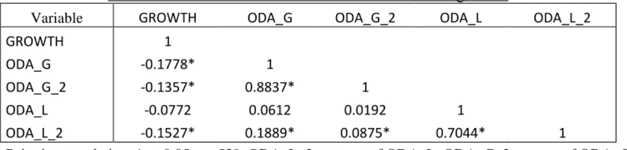
To complete the descriptive statistics section and to provide a starting point for the discussion in the next chapter, Table 2 shows the pairwise correlation coefficients between growth and the different bilateral aid variables.
Table 2 – Pairwise correlation between aid and growth
Variable GROWTH ODA_G ODA_G_2 ODA_L ODA_L_2
GROWTH 1
ODA_G -0.1778* 1
ODA_G_2 -0.1357* 0.8837* 1
ODA_L -0.0772 0.0612 0.0192 1
ODA_L_2 -0.1527* 0.1889* 0.0875* 0.7044* 1
Pairwise correlation, * p<0.05, n= 539, ODA_L_2 - square of ODA_L, ODA_G_2- square of ODA_G
Consistent with previous studies, the simple correlation between aid and growth is negative and significant (on the 5%-level), with a correlation coefficient of -0.18 for grants. The correlation between loans and growth is negative as well, but turns out to be statistically insignificant.13 However, the negative correlation between measures of aid and growth does not mean that aid in its various forms reduces growth. Instead, it is most likely the result of endogeneity bias due to reverse causality and omitted variables. The next section discusses these sources of bias and analyzes the most promising strategies to eliminate it, especially if the goal is to determine the differential impact of grants and loans.
4. Empirical strategy: How to overcome the endogeneity bias?
4.1 The problem
The main obstacle that every study of the aid-growth relationship has to overcome is the problem of the endogeneity of aid. Usually, the coefficient of foreign aid in a simple cross-country OLS growth regression has found to be negative. This does not necessarily mean that aid reduces growth. It rather reflects the simultaneity bias and shows that the dominant relationship between aid and growth is negative and runs from growth to aid (Roodman 2008). Countries with adverse shocks to growth receive more aid, and countries that grow unusually fast receive less aid as a
13 Out of the contemporaneous and squared aid terms, only loans fail to pass the threshold of r>|0.1|, which has
been proposed by Chatelain and Ralf (2014) to prevent spurious correlation in the presence of “classical surpressors.” However, the simple correlation coefficients for the lagged values are all below that threshold, making multicollinearity a serious concern.
16
percentage of GDP.14 This leads to a downward bias of the aid coefficient, which can be very
substantial. Again, this does not exclude the possibility of a causal relationship from aid to growth. But it shows that it is very challenging to uncover this causal effect and obtain significant and unbiased, not just spurious results, as it is shown for example by Brückner (2013). The research question addressed in this study intensifies this problem, because it essentially asks for the causal effect of aid on growth, conditional on the type of aid (as a concessional loan or a grant). The relationship between the type of aid and growth is expectedly highly endogenous as well, although the sign of the bias could go either way.
From a theoretical point of view, countries with bad growth performances may receive more grant aid (relative to loans) for simple altruistic reasons, i.e. because they are more in need of non-repayable funds. From the donor’s point of view, it would also make sense to give loans preferably to countries with good expected growth performances, as they are more likely to repay their debt in the future. This would both lead to a downward bias of grant aid relative to loan aid. However, one could also make the opposite argument, arguing that donors want to reward successful reforms in developing countries, preferably with grants, which may lead to an upward bias of grant aid. Even though the first strand of arguments (arguing for a downward bias of grant aid) is conceived to be theoretically stronger, the direction of the relative bias between grants and loans is ultimately an empirical matter.
The following sections will introduce and critically assess the main strategies that have been used to address the endogeneity of aid. Most importantly, it will be analyzed if and how these strategies can be used or extended to deal with the case of two endogenous regressors, being jointly determined and thus showing a potentially high degree of collinearity. The order in which these approaches are presented is somewhat ad-hoc, but one may argue that the identification strategies in the beginning are less complex and more efficient, but also more likely to give biased results than those considered in the end.
17
4.2 The different strategies to solve the endogeneity issue
4.2.1 Lags and differences: Clemens et al. (2012)
In choosing an identification strategy, there is often a tradeoff between robustness and efficiency. The most robust instruments are likely to be rather weak, leading to low statistical power. Clemens et al. (2012) choose an identification strategy which is simple and efficient, but only accounts for a part of the endogeneity problem. They use lagged values of aid as a regressor and transform all their data into first differences, which leads to the following equation to be estimated:
ΔGROWTHit = ΔODAit-1 + ΔODA_2it-1 + ΔLGDPit-1 + ΔXit +Period t + Δεit (2)
Using lagged aid flows as explanatory variables instead of contemporaneous flows has two positive effects. First, it accounts for the fact that aid may influence growth with a time lag, for example because investments need time until they become profitable. Thus, one would expect aid in period t-1 to have an impact on growth only in the next period t. The second effect is that lagging aid reduces the probability of simultaneity bias. While the growth performance of a recipient country may very well affect its aid inflows in the same period (especially if period averages are taken), it is less likely that it affects aid flows in the previous period.15
First-differencing the data also aims at reducing a part of the endogeneity bias that stems from omitted variables, by removing all country-specific time-invariant fixed effects (or confounding factors), as it can be seen in equation 2, where the variable Countryi from equation 1
cancelled out. However, first differencing and using lagged aid-flows are not a complete remedy against endogeneity bias. It is still possible that donor A increases its aid to recipient B, because it expects a negative growth shock in the next period. On the other hand, one could also imagine a case where the donor increases aid to recipient C, because a newly elected reform-oriented government will likely lead to a positive growth shock in the next periods. Hence, country-specific time-varying unobserved heterogeneity would still lead to an endogeneity bias, and the direction of the bias is not obvious. For this reason, Clemens et al. (2012) and other authors using the same identification strategy (for example Dreher, Minasyan, and Nunnenkamp (2014)) remain very cautious and only interpret their results as a positive correlation between aid and
18
growth, not necessarily a causal relationship.16 However, even this cautious interpretation has
been recently criticized by Roodman (2013, 2014), who replicates Clemens et al. and clearly lays out the strong exogeneity assumptions needed for unbiasedness of their results.17
4.2.2 Demand-side instruments: Burnside and Dollar (2000)
A more robust way to account for endogenous regressors than lagging and differencing is the use of instrumental variable (IV) estimators such as the two-stages least squares (2SLS) estimator. The idea of IV estimation (of which 2SLS and GMM are special cases) is to find one or more variables, called instruments, which are correlated with the endogenous regressor but are exogenous themselves. In other words, the instruments have to be relevant (highly correlated with the endogenous regressor) and valid (orthogonal, i.e. uncorrelated with the error term). They also have to satisfy the exclusion restriction, which is to say that they must not directly affect the dependent variable (only indirectly through the endogenous regressor), and thus can be left out in the final equation.
In their influential study, Burnside and Dollar (2000) chose instruments at the recipient country level, notably the logarithm of its population size, the share of arms imports in total imports and several interactions with their policy variable. There are two problems with this choice of instruments. The policy variable is very likely to be endogenous to growth, since it contains the inflation rate and the budget balance, which are both not orthogonal in a growth regression. Thus, policy-related instruments are probably invalid (Tarp and Hansen 2001). Furthermore, even though the recipient country’s population size may not directly influence growth, using it as an instrument does not necessarily satisfy the exclusion restriction. Bazzi and Clemens (2013) show that population size has been used as an instrument for various other variables, many of them being possibly related to growth. Unless those variables are all included in the growth regression (which would probably lead to an endogeneity bias on its own), the population size instrument will be correlated with the error term and thus violate the exclusion restriction. Since it has also been shown that the Burnside and Dollar IV strategy relies almost
16 Additionally, to increase the likelihood that they actually do capture some causal effects, Clemens et al. (2012)
exclude all aid flows that can only expected to have an impact on growth in the long run, thus using only „early-impact“ aid in their regressions.
19
completely on population size as an instrument,18 their IV results are not reliable and very likely
to be biased. In general, the main problem with their instrumentation strategy is that they pick instruments at the recipient country level, which makes them unlikely to be exogenous and to satisfy the exclusion restriction. In most cases, recipient level candidate instruments provide additional information about a country’s expected growth rate, and excluding them as regressors from the second stage inevitably leads to omitted variable bias. Lessmann and Markwardt (2012) extend the Burnside and Dollar strategy by adding instruments which should reflect the recipients past colonial relationship, for example the population share which has a European first language and several colonial relationship dummies. Both can expected to be correlated with aid, and may well be uncorrelated with growth. But even though this extension increases the instrumentation strength compared to the Burnside and Dollar benchmark, the results would still be biased, as long as the original instruments, which are not orthogonal to growth, are kept.
4.2.3 Supply-side instruments: Rajan and Subramanian (2008)
The state-of-the-art instrumentation strategy for aid picks instruments at the donor (and donor-recipient) level and hence models the supply of aid rather than its demand. Since instrumentation is mainly influenced by variables in the donor country, it can reasonably assumed to be exogenous to growth in the recipient country. Rajan and Subramanian (2008) have been the first to introduce this IV strategy, based on earlier work by Tavares (2003). The idea is to model each bilateral donor-recipient aid flow in a gravity equation, using colonial dummies and the population ratio between the two countries. It is assumed that a donor gives more aid to countries to which it has strong historical and cultural ties (represented by colony dummies) and over which it has a bigger influence (the population ratio). The predicted bilateral aid flows are aggregated over all donor countries and this “zero stage” aggregate is then used as a single instrument for aid in the first stage of the usual 2SLS procedure.
Because the second stage equation has as many excluded instruments as it has endogenous regressors and so is just identified, some specification tests such as the Hansen J-test are not implementable. Arndt, Jones, and Tarp (2010) show that the IV approach of Rajan and Subramanian can be improved in many ways. As in the Burnside and Dollar approach,
18 Clemens et al. (2012) show this by including population size in the second stage regression, which immediately
20
instrumentation strategy mainly relies on the population ratios (POPd/POPr). Furthermore, Arndt
et al. argue that donor-specific colonial variables are not orthogonal to growth and thus should be
excluded. For example, former colonies may have different institutions than other countries, which have a direct impact on the country’s growth prospects (Acemoglu, Johnson, and Robinson (2001)). However, another remedy for this problem is to substitute the donor-specific colonial dummies by a single colony dummy, leading to prefrred zero stage specification of Arndt et al.:
ODAdr = COLONYdr + LANGUAGEdr + ln(POPd/POPr) + COLONYdr*ln(POPd/POPr) (3)
+ Donord +
ε
drAs a further extension on Rajan and Subramanian, Arndt et al. also use different estimators, such as the Fuller (1977) modified Limited Information Maximum Likelihood (LIML) estimator, which shown to be more efficient than 2SLS if instruments are weak (Hahn, Hausman, and Kuersteiner (2004)). The supply-side IV approach has been criticized among others by Bazzi and Clemens (2013). They show that this identification strategy still relies almost completely on population size, similar to the demand-side approach discussed above. If population size is included as an instrument on its own, the instrument constructed in the zero stage loses all its statistical power.19 A recent contribution of Dreher, Eichenauer, and Gehring (2014) casts further
doubt on the supply-side instrumentation strategy of aid. They argue that this strategy only instruments the “geopolitically motivated” part of foreign aid, as it is based on donor-recipient ties. In their paper, they show that this geopolitically motivated aid is less effective in promoting growth than aid given without these motivations. 20 Thus, the supply-side instruments may not lead to unbiased IV estimates, because they instrument only a “selected part” of the sample of endogenous aid. The resulting coefficients should thus only be interpreted as local average treatment effects. While this may be a concern for general aid effectiveness regressions, it is less worrisome for the approach considered here, since it is mainly focused on the differential impact of grant aid and loan aid. If “geopolitically motivated” aid is as likely to be in the form of grants as in the form of loans, the loan-share coefficient will not be affected by this bias. One could argue that geopolitically motivated aid is much more likely to be in the form of grants than in the form of loans, because grants are more similar to a simple transfer. Thus, the grant aid coefficient
19 This might change once panel data is used and ideology is introduced as an additional instrument. Section 5 shows
whether this is the case.
21
would be upward-biased. However, the fact that grant aid might be more politically motivated and thus less effective than loan aid can be considered a part of the hypothesis that is tested in this paper. Hence, politically motivated aid supply is not a source of bias, but rather a “channel” through which grant aid could be more or less efficient than loan aid. The conclusion of Dreher, Eichenauer, and Gehring (2014) can be viewed as complementary to rather than competing with the analysis in this paper.
4.2.4 Quasi-experiments : Galiani et al. (2014)
Finally, the use of quasi-experiments is a different approach to achieve identification and estimate causal relationships when endogeneity issues are present. The distinctive feature of a quasi-experiment (or natural experiment) is that in most cases it uses just one, clearly exogenous binary shock, to identify a treatment effect.21 Because units of observation are observed before and after the shock (i.e. the treatment), the treatment basically divides those units into a treated and an untreated control group, very similar to actual experiments. But unlike in real experiments or in a randomized controlled trial (RCT), which is becoming more and more popular in economics, the treatment in quasi-experiments is not completely random. The treated group may have unobserved characteristics that make it different from the untreated group, even if no treatment would occur. If this is the case, the treatment assignment is endogenous, leading to a sample selection bias.
With regard to the effects of aid, the treatment or shock that is exploited can be either on the donors or on recipients of aid. Werker, Ahmed, and Cohen (2009) use large oil price shocks as an instrument to identify the effect of foreign aid given from rich Arab countries to poorer Muslim countries. They find no significant impact of aid on growth, but a strong positive effect on consumption and imports. Nunn and Qian (2014) show that US food aid, instrumented by shocks to US wheat production, increased the incidence, onset, and duration of civil war in the receiving countries.
The recent study of Galiani et al. (2014) uses a quasi-experimental approach with treatment at the recipient level to identify the effect of aid on growth. The natural experiment they employ
21 Estimation methods using a quasi-experimental approach are, for example, Differences-in-Differences, Regression
Discontinuity Design or Propensity Score matching. Instrumental variables estimation can also be used as a quasi-experiment, as it will be shown below.
22
as an instrument for aid is the crossing of the income threshold which is used by the International Development Association (IDA) to determine whether a country is eligible for aid. Once the per capita income of a receiving country is above this threshold, IDA aid flows are considerably reduced. Other multilateral aid agencies as well as bilateral donors use the IDA threshold as a signal for their own aid allocation as well. Thus, even though aid from IDA accounts on average for less than 10% of total aid, the crossing of the IDA threshold from below reduces aid inflows by a much larger percentage, due to the herding in aid allocation of donors. In the sample of Galiani et al. (2014) which includes 35 countries and the time from 1987-2009, aid decreased by a total of 59% after the threshold was crossed. A dummy which equals 1 when the recipient country’s per capita income is above the threshold and 0 otherwise should thus be strongly negatively correlated with aid inflows into the same country. Because of that, the “crossing” dummy is a candidate instrument for aid in the first stage of a 2SLS regression of growth on aid. In this case, one can speak of a quasi-experimental approach, because the IDA threshold, which is the cutoff that determines whether a country receives the treatment or not, is not chosen by the researcher or the country itself, and it is also not dependent on individual country characteristics. Instead, it is set exogenously by the World Bank (of which IDA is a member) and it is the same for all countries and over time, except for a yearly inflation adjustment.
However, the fact that the cutoff threshold is determined exogenously does not mean that the crossing of this cutoff is exogenous as well. If the crossing dummy is correlated with the error term in the growth regression, the results will be biased. This may for example be the case if a country crosses the threshold due to a few successive positive growth shocks, after which it will experience negative shocks that bring it back to its balanced growth path. In this case, the reduction of growth rates after the crossing will be falsely attributed to the reduction in aid, even though it only represents a usual reversion to the growth trend. Galiani et al. (2014) address this threat to their identification strategy in various ways. Most importantly, they develop a separate growth model and use it to predict the time of the IDA threshold crossing. By using the predicted rather than the actual crossing as an instrument for aid, they ensure that the instrument is not correlated with growth shocks and is thus completely exogenous. With this innovative and convincing approach, Galiani et al. (2014) find a comparatively large, significant, and robust positive effect of aid on growth. They further show evidence suggesting that aid increases growth via investment, at least in the short run. However, due to their quasi-experimental approach, they
23
can only include countries that have crossed the IDA threshold from below since 1987, leaving them with a rather homogenous sample of 35 countries. This homogeneity of the sample together with the relatively low number of countries make this approach not ideal for the purpose of this paper. But most importantly, since IDA gives both loans and grants, the crossing of the IDA threshold cannot be used to identify their differential effect on growth.
5. Results
The following section compares the results of several estimation strategies discussed in the previous chapter. To provide a starting point, the model is first estimated as a random effects panel estimator, which does not eliminate country-specific unobserved effects (Section 5.1). Those effects are subsequently eliminated by estimation in first differences (Section 5.2), following Clemens et al. (2012). Finally, a supply-side estimation strategy, in the tradition of Tavares (2003) and Rajan and Subramanian (2008), is implemented in an attempt to eliminate any remaining endogeneity bias (Section 5.3). Additional instrumentation and estimation strategies are then considered as robustness test, in Section 6.
5.1 Random effects
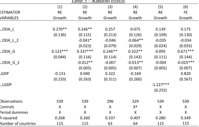
Table 3 shows the results of estimation of equation 1 (see Section 3) with the Feasible Generalized Least Squares (FGLS) estimator, thus assuming the Random effects model to be valid. As in all of the following estimations, a variance-covariance matrix which is robust to clustering at the country level is used. Period dummies are employed as well to capture period-specific shocks. Outliers are always identified and excluded according to the BACON algorithm introduced by Billor, Hadi, and Velleman (2000) (see also Weber (2010)). Until noted otherwise, the disaggregated aid variables (loans and grants) and later also their squared values are lagged by one period, to allow the aid flows to “work” and financed investments to materialize returns. Column 1 shows the results when loan aid and grant aid are simultaneously introduced into the growth regression, which implicitly assumes that they have a linear marginal effect on growth.
24
Table 3 – Random effects
(1) (2) (3) (4) (5) (6)
ESTIMATOR RE RE RE RE RE FE
VARIABLES Growth Growth Growth Growth Growth Growth
L.ODA_L 0.270** 0.246** 0.257 0.075 0.139 0.175 (0.136) (0.115) (0.213) (0.126) (0.109) (0.130) L.ODA_L_2 -0.041* -0.046 -0.064** -0.035 -0.034 (0.023) (0.079) (0.029) (0.024) (0.033) L.ODA_G 0.123*** 0.337*** 0.246** 0.322** 0.095 0.671*** (0.044) (0.116) (0.114) (0.143) (0.111) (0.144) L.ODA_G_2 -0.012** -0.007 -0.013** -0.004 -0.025*** (0.005) (0.005) (0.007) (0.005) (0.007) LGDP -0.131 0.040 0.322 -0.169 0.820 (0.233) (0.263) (0.311) (0.260) (0.567) L.LGDP -1.227*** (0.255) Observations 539 539 296 329 539 539 Controls X X X X† X X Period dummies X X X X X X R-squared 0.268 0.260 0.337 0.407 0.280 0.349 Number of countries 115 115 63 64 115 115 Robust standard errors in parentheses; *** p<0.01, ** p<0.05, * p<0.1; X†- time invariant controls added (geography, ethnic fractionalization, ICRG institution index, Sub-Saharan Africa and East Asia dummies); FE- Fixed effects; RE- Random effects; L- value lagged by one period
Both coefficients are positive and statistically significant. A one percentage point increase of loan aid is associated with a 0.27 percentage point increase in the growth rate. For grants, the respective increase equals 0.123 percentage points. The size of both coefficients is close to the typical marginal effect for aggregated aid that can be found in the literature.22 The linear marginal
effect of loans seems to be considerably higher than the effect of grants. However, the Wald test for the equality of coefficients cannot reject the hypothesis that both coefficients are in fact equal (p-value = 0.42). Furthermore, the results in Column 1 are most likely biased. A linear specification of both aid variables may lead to a misspecification bias, if their true effect on growth shows diminishing returns, as it is often found in the literature (see for example Hansen and Tarp, 2001). Hence, in Column 2 I introduce the squared values of loans and grants to account for this possibility. The fact that both squared terms have negative and significant
22 Clemens et al. (2012) find a marginal effect (at the sample average) between 0.1 and 0.2 percentage points,
Hansen and Tarp (2001) find approximately 0.1 percentage points with OLS, but a much larger effect with GMM (up to 1 percentage point). Galiani et al. (2014), who only consider a log-linear effect of aid on growth, find an increase of around 0.35 percentage points. Finally, Arndt, Jones, and Tarp (2014) find an effect ranging between 0.13 and 0.25 percentage points.
25
coefficients confirms the expectation that both types of aid seem to work with decreasing marginal returns. Again, both linear terms are positive and highly significant. But similarly to Column 1, the coefficients are not significantly different from each other (Wald test p-value = 0.56). The turning point, after which the effect of aid on growth becomes negative, is only around 3 percent of GDP for loan aid, which seems rather small. However, there are only 2 observations in the sample which show a higher average share of loans over GDP, annualized over a five-year period. For grants, the turning point is at 13 percent of GDP. Only 5 percent of the sample observations are above that threshold.
As in Column 1, the overall fit of the model in Column 2, most of the control variables are significant and all but have the expected signs (not shown). Column 3 restricts the sample to countries in the low-income and lower-middle-income group, according to the World Bank. It could be expected that aid works particularly well in these countries, since they face the strongest constraints to external financing sources, which aid could relieve. On the other hand, as they may lack sufficient financial institutions and absorption capacity, loan aid should work considerably less well than grants. Only the second of these assertions is illustrated in Column 3. The coefficients of loans and grants are both lower than with the full country sample, but only grant aid remains statistically significant.
The baseline specification contains only a time-varying set of control variables, because time-invariant regressors have to be omitted in the later steps, when the data are first-differenced. But up to this point, the random effects model allows the estimation of time-varying as well as time-invariant regressor. Thus, Column 4 adds an additional set of standard time-invariant controls, taken from Rajan and Subramanian (2008), to the baseline set of controls. The coefficients of grant aid and squared grant aid in Column 4 remain close to those in Column 2. The coefficient of loans, however, becomes insignificant, once time-invariant regressors are introduced.
This first, simple analysis seems to suggest that grants work better than loans, even though both types of aid have a tendency to be positively related to growth. But there are two main threats to the naïve identification strategy employed in this section. First of all, donor countries may jointly determine the amount of loans and grants that they give in a certain year, which would lead to a high correlation between loan aid and grant aid. Even more important, the aid
26
variables are highly correlated with their squared terms, relative to their correlation with growth (see Table 2). Chatelain and Ralf (2014) show that this multicollinearity problem, originating in the “suppressor variables” (i.e. the squared terms), can lead to a situation where identification of the true parameters becomes theoretically impossible. One way to detect multicollinearity is by calculating the Variance Inflation Factor (VIF) for the suspicious regressors. As a rule of thumb, VIFs larger than 10 indicate a severe multicollinearity problem (see for example Wooldridge 2013, p. 98). For the baseline regression of Column 2, this time estimated with OLS instead of random effects, none of the variables has such a high VIF. However, values between 7 and 9 for grants and squared grants indicate that multicollinearity may still be a problem to a certain degree. As an additional test, the so-called condition number is computed. Greene (2012, p.130) regards values higher than 20 as indicative of a multicollinearity problem, while Cameron and Trivedi (2005, p.350) set the threshold at 100. For the current specification, the condition number equals 6.4 and thus indicates no severe multicollinearity problem. However, following the suggestion of Chatelain and Ralf (2014), after which the suspicious “surpressors” may be dropped, I estimate most of the following specifications twice, with and without squared aid terms.
Another potential problem with the simple random effects model arises if unobserved country specific effect are present. The model assumes that those effects (captured by Countryi in
equation 1, Section 3) are purely random, i.e. completely uncorrelated with the error term ε it. However, in most cases this will not be the case, even with an extensive set of control variables. If there are unobserved effects which are correlated with the error term, the parameter estimates of the random effects model (estimated with FGLS) are biased (see Section 4.1). Hence, column 6 re-estimates the specification of column 2 on the within-transformed data, which eliminates part of the country-specific effects. A Hausman test shows that the models of columns 2 and 6 are significantly different from each other (at the 1%-level), implying that the Random effects estimates are inconsistent. Hence, the next section will use first-differenced data, which also removes the country-specific effects and thus tends to reduce the bias relative to the random effects model.
27
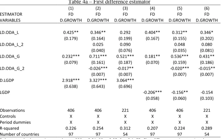
5.2 First-difference estimator
Table 4 shows the results of the estimation in first differences, following Clemens et al. (2012). Compared to the random effects panel data model, first-differencing has the advantage that it eliminates all unobserved (and observed), time invariant country-specific effects, reducing a possible endogeneity bias (see Section 4.2.1). The columns in Table 4 are organized similar to the first three columns in Table 3. First a linear effect of aid is assumed, then squared terms are introduced, and finally the sample is restricted to low-income countries.
The first three columns re-estimate the model of Table 3, now using first-differenced data. The coefficients of loans and grants show a similar pattern as before, although they are much larger now (comparable to the fixed effects version in Table 3, col. 6). Both are significant and positive in the linear specification, and loans seem more effective than grants. When quadratic terms are introduced, the grant coefficient becomes much larger, although both remain positive and significant. In this case, we can also determine that the coefficients of loans and grants are significantly different from each other (the Wald test returns a p-value of 0.0102). The turning point for aid is similar to the one found in Table 3, Column 2. Once the country sample is restricted, loans become insignificant. The controls have the expected sign (not shown), with one exception. The initial logarithm of GDP (in its first difference) is highly significant and positive in Columns 1 to 3. From a theoretical point of view, this seems counterintuitive, as it is usually thought of capturing convergence effects. But since the first difference of logarithmic initial GDP is simply the growth rate in period t-1, LGDPit-1 is now a lagged dependent variable and its
positive coefficient shows that growth rates are positively serially correlated. Unfortunately, the introduction of a lagged dependent variable, leads to the error term being correlated with the dependent variable.23 The whole estimation becomes inconsistent, and all parameter estimates are
potentially biased. This so-called Dynamic Panel or Nickell (1981) bias converges to zero if the number of periods goes to infinity. Hence, it is in particular a problem in relatively short panels.
23 This becomes obvious by looking at equation 2 and noting that ΔLGDP
it-1 = GROWTHit-1. This lagged dependent
variable is of course correlated with εit-1, and because this error term is a part of Δεit , ΔLGDPit-1 is endogenous in
28
Table 4a – First difference estimator
(1) (2) (3) (4) (5) (6)
ESTIMATOR FD FD FD FD FD FD
VARIABLES D.GROWTH D.GROWTH D.GROWTH D.GROWTH D.GROWTH D.GROWTH
LD.ODA_L 0.425** 0.346** 0.292 0.404** 0.312** 0.346* (0.179) (0.164) (0.199) (0.167) (0.155) (0.202) LD.ODA_L_2 0.025 0.090 0.048 0.080 (0.040) (0.076) (0.035) (0.081) LD.ODA_G 0.232*** 0.711*** 0.521*** 0.181** 0.536*** 0.431** (0.079) (0.161) (0.187) (0.070) (0.159) (0.186) LD.ODA_G_2 -0.026*** -0.017** -0.020*** -0.015** (0.007) (0.007) (0.007) (0.007) D.LGDP 2.918*** 3.327*** 3.064*** (0.638) (0.643) (0.696) LGDP -0.206*** -0.156** -0.154 (0.058) (0.060) (0.103) Observations 406 406 221 406 406 221 Controls X X X X X X Period dummies X X X X X X R-squared 0.226 0.254 0.312 0.207 0.224 0.289 Number of countries 97 97 54 97 97 54 Robust standard errors in parentheses; *** p<0.01, ** p<0.05, * p<0.1; FD- First difference estimator; L- value lagged by one period; D- value in first difference
There are different ways of addressing the Nickell bias. One naïve possibility would be to include only the level of LGDPit-1, not its first difference, which has been done in Columns 4 to 6. The
coefficient of LGDPit-1 (in its level) now has the “right” negative sign and is significant in two
out of three cases, while the aid variables are surprisingly robust to this specification change. However, the estimates can still not be expected to be unbiased, because the level of LGDPit is
obviously correlated with the differenced error term as well. Introducing the lagged difference of
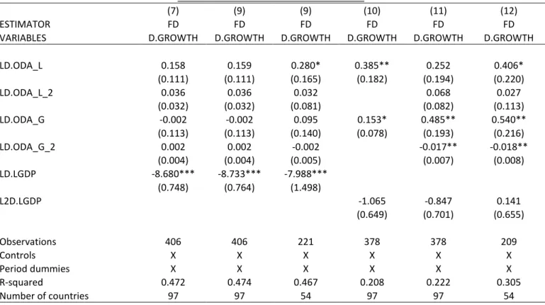
LGDPit-1 in Columns 7 to 9, as a proxy for the endogenous first difference, does also not
eliminate the bias completely. LGDPit-1 is still contained in the lagged difference, and is
correlated with the error term εit-1, contained in Δεit. Furthermore, almost all of the aid variables
become insignificant.
If instead the twice-lagged difference is used as a control, the aid regressors gain their significance again (Table 4b, Columns 10 to 12). This may be because the twice-lagged difference of LGDPit-1 is not correlated with the error term anymore, hence the dynamic panel
bias is completely eliminated. But it may also be because the twice-lagged difference is itself only marginally significant, and not a good proxy of the current (“un-lagged”) first difference.