Deep Learning and Structured Data
by
Chiyuan Zhang
B.E., Zhejiang University (2009)
M.E., Zhejiang University (2012)
Submitted to the Department of Electrical Engineering and Computer
Science
in partial fulfillment of the requirements for the degree of
Doctor of Philosophy
at the
MASSACHUSETTS INSTITUTE OF TECHNOLOGY
February 2018
© Massachusetts Institute of Technology 2018. All rights reserved.
Author . . . .
Department of Electrical Engineering and Computer Science
November 27, 2017
Certified by . . . .
Tomaso Poggio
Eugene McDermott Professor of Brain and Cognitive Sciences
Thesis Supervisor
Accepted by . . . .
Professor Leslie A. Kolodziejski
Professor of Electrical Engineering and Computer Science
Chair, Department Committee on Graduate Students
Deep Learning and Structured Data
by
Chiyuan Zhang
Submitted to the Department of Electrical Engineering and Computer Science on November 27, 2017, in partial fulfillment of the
requirements for the degree of Doctor of Philosophy
Abstract
In the recent years deep learning has witnessed successful applications in many different do-mains such as visual object recognition, detection and segmentation, automatic speech recogni-tion, natural language processing, and reinforcement learning. In this thesis, we will investigate deep learning from a spectrum of different perspectives.
First of all, we will study the question of generalization, which is one of the most fundamen-tal notion in machine learning theory. We will show how, in the regime of deep learning, the characterization of generalization becomes different from the conventional way, and propose alternative ways to approach it.
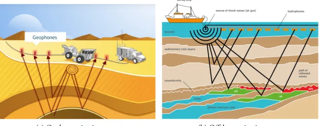
Moving from theory to more practical perspectives, we will show two different applications of deep learning. One is originated from a real world problem of automatic geophysical feature detection from seismic recordings to help oil & gas exploration; the other is motivated from a computational neuroscientific modeling and studying of human auditory system. More specifi-cally, we will show how deep learning could be adapted to play nicely with the unique structures associated with the problems from different domains.
Lastly, we move to the computer system design perspective, and present our efforts in build-ing better deep learnbuild-ing systems to allow efficient and flexible computation in both academic and industrial worlds.
Thesis Supervisor: Tomaso Poggio
Acknowledgments
First of all, I would like to thank all the people who brought me to the field of machine learning and academic research, especially Dr. Xiaofei He, Dr. Deng Cai and Dr. Binbin Lin and all the other people at the zju-learning group in Zhejiang University. Without them, I would never have made up my mind to go abroad and pursue a PhD, and I would have totally missed this great journey of the past five years in my life. It is still hard to believe that I am already near the end of it now.
I would like to thank my advisor Dr. Tomaso Poggio, who offered me the opportunity to be in the great family of the poggio-lab. Tommy always has a great vision in bridging the understandings of the foundations of machine learning systems and human intelligence. I would have been completely lost without his guidance. On the other hand, he is also very supportive and gives me great freedom to explore and learn to do independent research, as well as pursuing a colorful life apart from study.
I would like to thank my great thesis committee, Dr. Piotr Indyk, Dr. Tommi Jaakkola and Dr. Stefanie Jegelka. All of them not only directly gave me valuable advices and comments on the thesis, but also influenced me in other occasions during my graduate study. I started my PhD on a collaborative project with Shell Oil, and Piotr was the leading Principal Investigator in the team. Piotr has always been a great inspiration for me since then. One of the first class I took at MIT was 6.438, taught by Tommi. Tommi is a great teacher and everything I learned in the class has laid a solid foundation for the rest of my pursuit. I also came to interact with Stefanie initially through a class, and she continued to offer valuable feedbacks afterwards and the conversations directly influenced part of my thesis projects.
I’m grateful to all the other members of the Poggio-lab. Dr. Lorenzo Rosasco is essentially the second advisor to me. His sharp opinions has shaped my mind of critical and mathematical thinking. Gadi Geiger has also become a mentor as well as a good friend throughout our daily coffee chat. Youssef Mroueh was my CSAIL buddy and a valuable source of research advices and friendship. Andrea Tacchetti and Yena Han both offered invaluable friendships and inspi-rations for life. Many thanks to Fabio Anselmi, Guillermo D. Canas, Carlo Ciliberto, Georgios Evangelopoulos, Charlie Frogner, Leyla Isik, Joel Z. Leibo, Owen Lewis, Qianli Liao, Ethan
Meyers, Brando Miranda, Jim Mutch, Yuzhao (Allen) Ni, Maximilian Nickel, Gemma Roig Noguera, and Stephen Voinea for their help and many interesting and insightful conversations. Special thanks to our administrative assistant Kathleen Sullivan for all the helps and donuts and for introducing me to inktober.
I’m extremely fortunate to have the chance to interact with many other great people at MIT. Thanks to Dr. Afonso Bandeira, Dr. Jim Glass, Dr. Leslie Kaelbling, Dr. Ankur Moitra, Dr. Sasha Rakhlin, Dr. Philippe Rigollet. I’m also grateful for the invaluable experiences working with wonderful people outside MIT during internships and visitings. Many thanks to Dr. Samy Bengio, Dr. Marco Cuturi, Dr. Moritz Hardt, Dr. Detlef Hohl, Dr. Sugiyama Masashi, Dr. Mauricio Araya Polo, Dr. Neil Rabinowitz, Dr. Ben Recht, Dr. Francis Song, Dr. Ichiro Takeuchi and Dr. Oriol Vinyals.
A very special gratitude goes out to Shell R&D, the Nuance Foundation, and the Center for Brain, Minds and Machine for providing research funding. All this would be impossible without their generous support.
I’m also grateful to all the friends, old an new, who have supported me along the way. Special thanks to Tianqi Chen, Xinlei Chen, Louis Chen, Xinyun Chen, Fei Fang, Xue Feng, Siong Thye Goh, Chong Yang Goh, Xuanzong Guo, Sonya Han, Daniel “Shang-Wen” Li, Duanhui Li, Chengtao Li, Mu Li, Song Liu, Tengyu Ma, Hongyao Ma, Yao Ma, He Meng, Yin Qu, Ling Ren, Ludwig Schmidt, Peng Wang, Shujing Wang, Zi Wang, Xiaoyu Wu, Jiajun Wu, Bing Xu, Tianfan Xue, Cong Yan, Judy “Qingjun” Yang, Xi Yang, Wei Yu, Zhou Yu, Wenzhen Yuan, Yu Zhang, Zhengdong Zhang, Xuhong Zhang, Sizhuo Zhang, Shu Zhang, Ya Zhang, Hao Zhang, Xijia Zheng, Qinqing Zheng, Bolei Zhou, and many others. They have become an essential part for my research, study and life. I will miss the study groups, the board games, the hikings, the day trips, and the home-made hot pots.
A special thanks to Sam Madden, my academic advisor, and Janet Fischer, our EECS Grad-uate Administrator, who are always kind and patient and knowledgeable to help and make sure everything is going on well with my study and academic life.
And finally, last but by no means least, I want to dedicate the thesis to my mother Hua Wang and my father Zhongmo Zhang, for their love and for fostering all my academic endeavors.
Contents
1 Introduction 12
1.1 Main contributions . . . 14
2 Understanding generalization in deep learning 15 2.1 Backgrounds and problem setup . . . 16
2.1.1 Rademacher complexity and generalization error . . . 21
2.2 Related work on the three major theoretical questions in deep learning . . . . 24
2.2.1 Approximation error . . . 24
2.2.2 Optimization error . . . 25
2.2.3 Generalization error . . . 27
2.3 Some puzzles in understanding deep learning . . . 28
2.4 Understanding deep learning requires rethinking generalization . . . 31
2.4.1 Our contributions . . . 32
2.4.2 Related work . . . 35
2.4.3 Effective capacity of neural networks . . . 36
2.4.4 The role of regularizers . . . 39
2.4.5 Finite-sample expressivity . . . 43
2.4.6 Implicit regularization: an appeal to linear models . . . 44
2.4.7 Conclusion . . . 46
2.4.8 Appendix . . . 47
2.5.1 Flat minimizers . . . 53
2.5.2 Margins and other noise conditions . . . 55
2.5.3 Norms and complexity measures . . . 57
3 Application and adaptation of deep learning with domain structures 59 3.1 Learning based automatic geophysical feature detection system . . . 60
3.1.1 Petroleum exploration and seismic survey . . . 60
3.1.2 Related work on automatic geophysical feature detection . . . 62
3.1.3 Deep learning based fault detection from raw seismic signals . . . 62
3.1.4 Learning with a Wasserstein distance . . . 72
3.2 Invariant representation learning for speech and audio signals . . . 98
3.2.1 Backgrounds . . . 100
3.2.2 Related work . . . 101
3.2.3 A formal group-invariant representation and ConvNets based approx-imation . . . 102
3.2.4 Empirical studies . . . 108
4 Building flexible and efficient deep learning systems 117 4.1 The importance of high quality deep learning systems and related work . . . . 117
4.2 MXNet: flexible and efficient deep learning library for distributed systems . . . 123
4.2.1 Introduction. . . 123 4.2.2 Programming interface . . . 124 4.2.3 Implementation . . . 127 4.2.4 Evaluation . . . 129 5 Conclusion 132 5.1 Summary . . . 132 5.2 List of contributions . . . 133
List of Figures
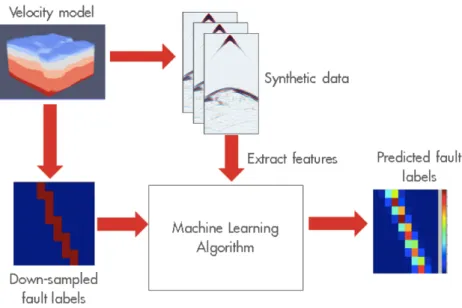
2-1 Illustration of feedforward neural network architectures. . . 16
2-2 Example of training curves on CIFAR-10. . . 30
2-3 Fitting random labels and random pixels on CIFAR-10. . . 37
2-4 Effects of implicit regularizers on generalization performance. . . 42
2-5 The network architecture of the Inception model adapted for CIFAR-10. . . . 48
2-6 The training accuracy on the convex interpolated weights of three different (global) minimizers found by SGD via different random initialization. Each subfigure shows the interpolated plot on different dataset with either true labels or random labels. . . 54
3-1 Illustrations of seismic surveys. . . 60
3-2 Illustrations of faults. . . 63
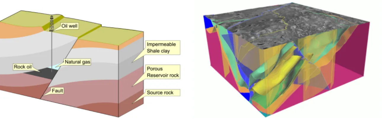
3-3 Workflow of a machine learning based fault detection system. . . 64
3-4 Example of a randomly generated velocity model with a multiple faults. . . 65
3-5 Illustration of the benefits of the Wasserstein loss. . . 68
3-6 Visualization of a 3D velocity model, its fault location and our predictions. . . 69
3-7 A second visualization of a 3D velocity model, its fault location and our pre-dictions. . . 70
3-8 Example of two images from two different categories in ImageNet. . . 73
3-9 Illustration of the Wasserstein loss with the lattice example. . . 74
3-11 MNIST example for learning with a Wasserstein loss. . . 81
3-12 Top-K cost comparison of the proposed loss (Wasserstein) and the baseline (Divergence). . . 83
3-13 Trade-off between semantic smoothness and maximum likelihood. . . 84
3-14 Examples of images and tag predictions in the Flickr dataset. . . 84
3-15 Illustration of training samples on a 3x3 lattice with different noise levels. . . . 94
3-16 Full figure for the MNIST example. . . 95
3-17 More examples of images and tag predictions in the Flickr dataset. . . 96
3-18 More examples of images and tag predictions in the Flickr dataset. . . 97
3-19 Illustration of the speech generation and recognition loop.. . . 99
3-20 The word “park” spoken by different speakers. . . 99
3-21 Illustration of the approximation of the group orbits. . . 105
3-22 Illustration of simple-complex cell based network architecture. . . 106
3-23 Illustration of the phone classification experiment.. . . 108
3-24 Phone classification error rates on TIMIT. . . 109
3-25 Illustration of VTL invariance based network architecture. . . 113
3-26 Training cost and dev set frame accuracy against the training iterations on the TIMIT dataset. . . 114
3-27 Performance of models trained on original and VTL-augmented TIMIT. . . . 116
4-1 Illustration of the architecture and computation graph forMXNet. . . 127
4-2 ComparingMXNetwith other systems for speed on a single forward-backward pass. . . 129
4-3 Memory usage comparison for different allocation strategies. . . 130
List of Tables
2.1 List of the number of parameters vs. the number of training examples in some
common models used on two image classification datasets. . . 31
2.2 List ofp/n(number of parameters over number of training samples) ratio and classification performance on a few over-parameterized architectures on CIFAR-10. . . 32
2.3 The training and test accuracy of various models on CIFAR-10. . . 40
2.4 The accuracy of the Inception v3 model on ImageNet. . . 49
2.5 Generalizing with kernels. . . 51
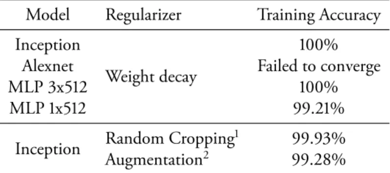
2.6 Results on fitting random labels on the CIFAR-10 dataset with weight decay and data augmentation. . . 52
3.1 Results of the fault localization experiments. . . 68
3.2 Phone classification error rate using different invariance modules. . . 111
Underfull \hbox (badness 10000) in paragraph at lines 88–88
—LATEX
1
Introduction
Machine learning covers a wide range of methods to extract useful patterns from a dataset that is usually assumed to be samples from an unknown probability distribution. Supervised learning, one of the main setup in machine learning, is formulated as finding a function f such that the expected loss Ez[ℓ(f, z)] over the random variable z representing the data is minimized. The basic setting is that the distribution for the input random variable z is unknown, but we have access to a training set of n i.i.d. samples S ={z1, . . . , zn}. As a result, the problem is usually
approached by solving the following Empirical Risk Minimization (ERM) problem,
min f∈F ˆ ES[ℓ(f, z)] := min f∈F 1 n n ∑ i=1 ℓ(f, zi) (1.1)
And then provide certificates showing that a “reasonable good” solution to this problem is also “reasonably good” for the original (expected) loss. Here F is a hypothesis space of candidate
functions that we choose a priori to seeing the data. A trade off on how good the best candidate inF could perform (the bias) and how close the solution we found by ERM to the optimal solution under the expected loss (the variance) will decide the optimal choice ofF. In practice, other concerns such as what algorithm to use to solve (1.1) will also affect the choice ofF.
Before the wide adoption of deep learning, people heavily rely on the nice property of con-vexity in both optimization and statistical theory, and tend to chooseF to be linear functions in some (predefined) feature spaces, and use convex surrogate losses to solve the ERM problems.
On the other hand, with deep neural networks,F consists of hypotheses that are defined through composition of linear maps and component-wise non-linear activations. The optimiza-tion problem (1.1) becomes non-convex even with a convex loss ℓ. While analyzing both the optimization dynamics and the statistical behavior become harder in this setting, empirically, this formulation drastically improves the state-of-the-art performance in real world problems from various domains such as computer vision [Krizhevsky et al., 2012, Russakovsky et al.,
2015,He et al.,2016,Taigman et al.,2014,Ren et al.,2015], speech recognition [Hinton et al.,
2012b, Chan et al., 2016, Amodei et al., 2016], natural language processing [Sutskever et al.,
2011, Bahdanau et al.,2015a, Sutskever et al., 2014], and reinforcement learning [Mnih et al.,
2015,Silver et al.,2016], just to name a few.
The success of deep learning inspired a spectrum of different research topics from theoretical understanding, to applying and adapting deep neural networks to the structures of specific tasks, to building high performance deep learning systems. In this thesis, we compile different projects that the author has worked on at different stages to provide a systematic view from the three different perspectives.
Specifically, in Chapter 2, we will talk about our efforts on the theoretical aspects about understanding the generalization of deep learning. Chapter3 consists of two applications of deep learning with adaptations to the domain specific structures arise in the each of the applica-tion scenarios. Chapter4is devoted to building high performance deep learning systems. The detailed problem setup and backgrounds will be provided in each chapter, respectively. Finally, we will conclude with a summary and a list of contributions in Chapter5.
1.1
Main contributions
We summarize the main contributions of this thesis into three parts. A full list of publications and softwares included in this thesis is shown in section5.2.
Theory we studied the theoretical aspects of the generalization behavior of large scale deep
neural networks, and revealed some puzzling behavior in the regime of deep learning that makes it hard to directly apply the conventional distribution free analysis from the statistical learning theory toolkits [Zhang et al.,2017a].
Application We applied deep learning to two different problems: automatic geophysical
fea-ture detection [Zhang et al.,2014b,Dahlke et al.,2016,Araya-Polo et al.,2017] and invariant representation learning for speech and audio signals [Zhang et al., 2014a,c,2015b]. The deep learning framework is adapted to the domain specific structures of the data and task in those two problems. Beside successfully applying deep learning algorithms, we also get new insights to the design of the convolutional neural network architectures [Zhang et al.,2015b] and new algorithms for learning with output structures [Zhang et al.,2015a].
System we built efficient deep learning toolkits [Chen et al., 2015b, 2016] to support our own research and also make it general purpose to support to the deep learning use cases in both academia and industry. Our open source project MXNet has an efficient asynchronized computation engine written in C++, built-in distributed computation support and supports a wide range of front end interface languages including Python, Julia, R, and Scala. It is widely recognized and adopted by the community, chosen to be the main deep learning system for Amazon AWS cloud computing platform and integrated by the NVidia GPU Cloud as one of the six major deep learning platforms.
2
Understanding generalization in deep
learning
Generalization is a fundamental notion in machine learning and a central topic in statistical and computational learning theory. In Section 2.1, we will formally define the problem and provide a basic introduction to the existing literature. In Section2.2, by summarizing the existing liter-ature of learning theoretical studies, we will see how the major theoretical questions in learning can be summarized into three core components that studies approximation error, optimization error and generalization error, respectively. Among thouse, we will show in Section2.3some examples of puzzles in our theoretical understanding that are unique to the regime of deep learning. Finally, in Section2.4, we provide a systematic study of the generalization behaviors in the regime of deep learning. To conclude this chapter, we discuss future work and recent progresses in Section2.5.
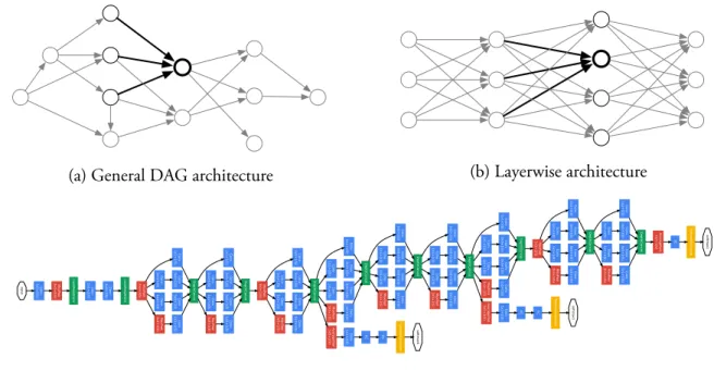
(a) General DAG architecture (b) Layerwise architecture • A linear layer with softmax loss as the classifier (pre-dicting the same 1000 classes as the main classifier ,b ut remo ved at inference time). A schematic vie w of the resulting netw ork is depicted in Figure 3. 6. Training Methodology GoogLeNet netw orks were trained using the DistBe-lief [4] distrib uted machine learning system using mod-est amount of model and data-parallelism. Although we used a CPU based implementation only , a rough estimate suggests that the GoogLeNet netw ork could be trained to con ver gence using fe w high-end GPUs within a week, the main limitation being the memory usage. Our training used asynchronous stochastic gradient descent with 0.9 momen-tum [17], fix ed learning rate schedule (decreasing the learn-ing rate by 4% ev ery 8 epochs). Polyak av eraging [13] w as used to create the final model used at inference time. Image sampling methods ha ve changed substantially ov er the months leading to the competition, and already con ver ged models were trained on with other options, some-times in conjunction with changed hyperparameters, such as dropout and the learning rate. Therefore, it is hard to gi ve a definiti ve guidance to the most ef fecti ve single w ay to train these netw orks. To complicate matters further ,some of the models were mainly trained on smaller relati ve crops, others on lar ger ones, inspired by [8]. Still, one prescrip-tion that w as verified to w ork very well after the competi-tion, includes sampling of various sized patches of the im-age whose size is distrib uted ev enly between 8% and 100% of the image area wi th aspect ratio constrained to the inter -val [3 4, 4 3 ]. Also, we found that the photometric distortions of Andre w Ho w ard [8] were useful to combat ov erfitting to the imaging conditions of training data. 7. ILSVRC 2014 Classification Challenge Setup and Results The ILSVRC 2014 classification challenge in volv es the task of classi fying the image into one of 1000 leaf-node cat-egories in the Imagenet hierarch y. There are about 1.2 mil-lion images for training, 50,000 for validation and 100,000 images for testing. Each image is associated with one ground truth cate gory ,and performance is measured based on the highest scoring classifier predictions. Tw o num-bers are usually reported: the top-1 accurac y rate, which compares the ground truth ag ainst the first predicted class, and the to p-5 error rate, which compares the ground truth ag ainst the first 5 predicted classes: an image is deemed correctly classified if the ground truth is among the top-5, re gardless of its rank in them. The challenge uses the top-5 error rate for ranking purposes. in pu t Co n v 7x 7+ 2( S) Ma x Po o l 3x 3+ 2( S) Lo ca lR e spN o rm Co n v 1x 1+ 1( V ) Co n v 3x 3+ 1( S) Lo ca lR e spN o rm Ma x Po o l 3x 3+ 2( S) Co n v 1x 1+ 1( S) Co nv 1x 1+ 1( S) Co n v 1x 1+ 1( S) Ma x P o ol 3x 3+ 1( S) De p thC o n cat Co nv 3x 3+ 1( S) Co n v 5x 5+ 1( S) Co n v 1x 1+ 1( S) Co n v 1x 1+ 1( S) Co nv 1x 1+ 1( S) Co n v 1x 1+ 1( S) Ma x P o ol 3x 3+ 1( S) De p thC o n cat Co nv 3x 3+ 1( S) Co n v 5x 5+ 1( S) Co n v 1x 1+ 1( S) Ma x Po o l 3x 3+ 2( S) Co n v 1x 1+ 1( S) Co nv 1x 1+ 1( S) Co n v 1x 1+ 1( S) Ma x P o ol 3x 3+ 1( S) De p thC o n cat Co nv 3x 3+ 1( S) Co n v 5x 5+ 1( S) Co n v 1x 1+ 1( S) Co n v 1x 1+ 1( S) Co n v 1x 1+ 1( S) Co n v 1x 1+ 1( S) Ma x P oo l 3x 3+ 1( S) Av e rage P oo l 5x 5+ 3( V ) De p thC o n cat Co n v 3x 3+ 1( S) Co n v 5x 5+ 1( S) Co n v 1x 1+ 1( S) Co n v 1x 1+ 1( S) Co n v 1x 1+ 1( S) Co nv 1x 1+ 1( S) Ma x Po o l 3x 3+ 1( S) De p thC on cat Co n v 3x 3+ 1( S) Co nv 5x 5+ 1( S) Co n v 1x 1+ 1( S) Co n v 1x 1+ 1( S) Co n v 1x 1+ 1( S) Co nv 1x 1+ 1( S) Ma x Po o l 3x 3+ 1( S) De p thC on cat Co n v 3x 3+ 1( S) Co nv 5x 5+ 1( S) Co n v 1x 1+ 1( S) Co nv 1x 1+ 1( S) Co n v 1x 1+ 1( S) Co n v 1x 1+ 1( S) Ma x Po o l 3x 3+ 1( S) Av e rag e Po o l 5x 5+ 3( V ) De p th Co n cat Co n v 3x 3+ 1( S) Co n v 5x 5+ 1( S) Co n v 1x 1+ 1( S) Ma x P oo l 3x 3+ 2( S) Co n v 1x 1+ 1( S) Co n v 1x 1+ 1( S) Co n v 1x 1+ 1( S) Ma xP o ol 3x 3+ 1( S) De p thC o n cat Co n v 3x 3+ 1( S) Co n v 5x 5+ 1( S) Co n v 1x 1+ 1( S) Co n v 1x 1+ 1( S) Co n v 1x 1+ 1( S) Co n v 1x 1+ 1( S) Ma xP o ol 3x 3+ 1( S) De p thC o n cat Co n v 3x 3+ 1( S) Co n v 5x 5+ 1( S) Co n v 1x 1+ 1( S) Av e rag e Po o l 7x 7+ 1( V ) FC Co n v 1x 1+ 1( S) FC FC So ftm ax A ct iva tion so ftm ax 0 Co n v 1x 1+ 1( S) FC FC So ft m a x A ctiv a tio n so ft m a x 1 So ftm a x A ctiv a tio n so ft m a x 2 Figure 3: GoogLeNet netw ork with all the bells and whistles.
(c) The GoogLeNet architecture [Szegedy et al.,2015]
Figure 2-1: Illustration of feedforward neural network architectures.
2.1
Backgrounds and problem setup
Deep learning is generally referred to as any machine learning related techniques that uses “deep” neural networks — neural networks that have more than one hidden layers. In this thesis, we specifically focus on supervised learning, as formalized in Chapter1, and we will be primarily studying the feedforward neural networks.
A feedforward neural network is a parametric function fθG : Rd → Rk, where d and k are
input and output dimensions, respectively. HereG is a directed acyclic graph (DAG) describing the architecture of the neural network, which maps from the input nodes to the output nodes. As illustrated by Figure2-1a, the computation at a vertex v is defined as
xv = σ ∑ u:(u→v)∈G θu→vxu (2.1)
where σ : R → R is a non-linear activation function, which is typically chosen to be the sigmoid function σ(x) = 1/1+e−x or the Rectified Linear Units (ReLUs) σ(x) = max(x, 0).
The parameters{θu→v : (u→ v) ∈ G} associated with are called the “weights” of the network.
2-1b. The nodes in each layer receive only connections from the previous layer. This kind of architecture can be easily described by composition of linear transforms and componentwise nonlinear activations. For example, a L-layer feedforward neural network can be described in either of the two ways:
xi,j = σi ( ∑ k wijkxi−1,k ) , i = 1, . . . , L (2.2) xi = σi ( Wixi−1), i = 1, . . . , L (2.3)
where the activation function σi(·) is applied componentwise for vector inputs. Now the
net-work weights θ are the collection of linear transformation coefficients {wijk} or {Wi}, with
x = x0being the input and y = xLbeing the output. We use a layer index i for the activation
function because conventionally, the output layer does not use an activation function, or uses the identity activation.
The architecture with a simple chain of densely connected layers is usually called multi-layer
perceptrons (MLPs). Usually, each layer could have its own structure. For example, a
convolu-tional layer, commonly used in computer vision tasks, organize its nodes as a spatial grid. Each node is only sparsely connected to the surrounding nodes from the previous layer, and share the weights with other nodes in the same layer. It is very common to take those basic layers (as oppose to nodes) as building blocks and design a DAG to represent the computation. Figure 2-1cshows the “GoogLeNet” or “Inception” architecture proposed bySzegedy et al.[2015] as an example. Modern network architectures could easily have hundreds to thousands of computa-tional layers [He et al.,2016], with auxiliary components for normalization [Ioffe and Szegedy,
2015] and transformations [Jaderberg et al.,2015], recurrent connections with attentions [ Bah-danau et al.,2015b], gates [Chung et al.,2014] and differentiable memory [Graves et al.,2014], and number of parameters ranging from 105to 1012[Shazeer et al.,2017].
Our goal is to study the practice of using deep neural networks (of a specific architecture) as the hypothesis for solving the supervised learning problems. Specifically, we assume an al-gorithm A is used to solved the ERM problem (1.1). Given a training set S = {z1, . . . , zn},
following definitions exists1: ˆ ES[ℓ( ˆfS, z)] = min f∈F ˆ ES[ℓ(f, z)] (2.4) Ez[ℓ(fF, z)] = min f∈FEz[ℓ(f, z)] (2.5) Ez[ℓ(f⋆, z)] = min f Ez[ℓ(f, z)] (2.6)
For classification problems, f⋆ is usually called the Bayes classifier, and achieves the minimum
possible loss among all the deterministic functions. E[ℓ(f⋆, z)]is called the Bayes error,
repre-senting the intrinsic difficulty of the problem, and commonly used as the baseline performance for analyzing a learning algorithm. fF is the optimal model inF for the expected loss, while
ˆ
fSis the optimal model for the empirical loss on the training set S.
A common way of analyzing the loss of a learned model ˆfA,S is through the following bias-variance decomposition:
E[ℓ( ˆfA,S, z)] = E[ℓ( ˆfA,S, z)]− E[ℓ(fF, z)]
| {z }
estimation error / variance
+ E[ℓ(f| F, z)]{z− E[ℓ(f⋆, z)]}
approximation error / bias
+ E[ℓ(f| {z }⋆, z)]
Bayes error
(2.7)
The Bayes error is intrinsic to the problem, and beyond our control. The approximation error describes how well F could approximate the optimal Bayes classifier f⋆. Larger F leads to
smaller approximation error. On the other hand, the estimation error characterize how well the algorithm A, when given only the training set S as a proxy to the underlying unknown data distribution, could be able to find the best model fF inF. Due to the discrepancy between
the empirical loss and the expected loss, usually largerF makes the problem harder. As a result, there is a bias-variance trade-off in the size / complexity ofF.
In statistical learning theory, the algorithm A is usually assumed to be the ERM estimator. In other words, ˆfA,S = ˆfS. However, in some cases, for example, when ℓ(f, (x, y)) = I[f (x)̸=
y] is the binary classification loss, it is not computationally efficient to compute the ERM estimator. Even when the ERM problem (1.1) is convex, most of the existing methods can only guarantee an ε-approximate solution for a finite time budget. Therefore, we distinguish
1For the brevity of notation, we also assume the minimizers are unique. Most of the conclusions could be
between ˆfA,S and ˆfSand make the following decomposition instead:
E[ℓ( ˆfA,S, z)] = E[ℓ( ˆfA,S, z)]− ˆE[ℓ( ˆfA,S, z)] + ˆE[ℓ( ˆfA,S, z)]− ˆE[ℓ( ˆfS, z)] +
ˆ
E[ℓ( ˆfS, z)]− E[ℓ(fF, z)] + E[ℓ(fF, z)]− E[ℓ(f⋆, z)] + E[ℓ(f⋆, z)]
= ˆE[ℓ( ˆfA,S, z)]− ˆE[ℓ( ˆfS, z)]
| {z }
optimization error
+ E[ℓ(fF, z)]− E[ℓ(f⋆, z)]
| {z }
approximation error / bias
+ E[ℓ(f⋆, z)]
| {z } Bayes error + E[ℓ( ˆfA,S, z)]− ˆE[ℓ( ˆfA,S, z)] + ˆE[ℓ( ˆfS, z)]− E[ℓ(fF, z)]
(2.8)
where the last four terms can be bounded via
E[ℓ( ˆfA,S, z)]− ˆE[ℓ( ˆfA,S, z)] + ˆE[ℓ( ˆfS, z)]− E[ℓ(fF, z)]
≤ E[ℓ( ˆfA,S, z)]− ˆE[ℓ( ˆfA,S, z)] + ˆE[ℓ( ˆfF, z)]− E[ℓ(fF, z)] ≤ 2 sup f∈F ˆE[ℓ(f, z)] − E[ℓ(f, z)] | {z } generalization error (2.9)
The generalization error, sometimes also referred to as the generalization gap, is decided by the difference between the expected loss and the empirical loss. It is easy to see largerF will increase the generalization error, and the trade-off in choosing F is now between the approximation error and generalization error.
Furthermore, the optimization error, which characterize how well we can solve the ERM problem (1.1), could also depend on F in complicated ways. For convex optimization, the convergence is well understood [Bubeck,2015]. On the other hand, non-convex optimization in machine learning is a very active research topic today [Zheng and Lafferty,2015,Sun et al.,
2015,Montanari,2016,Raginsky et al.,2017,Zhang et al.,2017b], and for the most general case of training large neural networks, it is still not very clear why we are empirically so successful at solving those non-convex problems.
Note upper bounding by the supf∈F seem to be very loose. However, since both ˆfA,Sand ˆ
Edepend on the data, one needs some way to decouple the dependency for the ease of analysis. Usually this upper bound is already good enough to provide useful sufficient condition for learnability. In the distribution free setting, where the learning algorithm is required to work well with all possible data distributions, it can be shown that this upper bound is actually tight.
Various ways to control (2.9) usually reduce to bounds of the order O(d˜/n) ∼ O(√d˜/n),
where ˜d is some complexity measure for the hypothesis space F. A high level idea of the general arguments used here is: for any given f , by the law of large number, under appropriate conditions such as boundedness, one can show that the empirical average ˆE[ℓ(f, z)]converges to the expectation E[ℓ(f, z)] with high probability. However, to deal with supf∈F, one need
to make sure every f ∈ F converges uniformly. When F is finite, this can be controlled by a simple union bound, which leads to a uniform convergence bound with a multiplier log|F|. When |F| = ∞, this bound becomes trivial. In this case, one need employ a more clever union bound where “similar” functions inF are grouped together and “counted” once. The exact notion of “similarity” depends on what kind structures ofF are available. For example, if
F is a metric space with an appropriate metric, one can treat functions within an ε metric ball
as “similar” and use the covering number ofF to represent the complexity [Cucker and Smale,
2002]. Another example is in binary classification, when evaluated on a given finite dataset
S = (z1, . . . , zn)of n points, there are at most 2npossible unique outcomes:
|FS| = |{f(z1, . . . , zn) : f ∈ F}| ≤ 2n
as a lot of functions are mapped to the same n-dimensional binary vectors. We get |FS| <
∞, but O(√log|FS|/n) = O(1) is still not good enough for a useful generalization bound.
When some structures inF is known that allows us to argue about the combinatorial properties of|FS|, such that it grows slower than 2n, a meaningful bound can be provided. The notion of
Vapnik-Chervonenkis (VC) dimension allows us to bound|FS| by O( ˜dn)for n > ˜d. Therefore,
if F has VC dimension ˜d, then the generalization bounds can be reduced to O(√d log n˜ /n).
Please refer to the books such asKearns and Vazirani[1994],Mohri et al.[2012],Shalev-Shwartz and Ben-David[2014] for detailed developments of the upper bounds and lower bounds for generalization error.
For completeness, we provide a brief overview of the standard arguments through the
2.1.1 Rademacher complexity and generalization error
For simpler notion, let us define the loss classL = {z 7→ ℓ(f, z) : f ∈ F}. The generalization error we want to bound is
sup
l∈L
ˆES[l(z)]− Ez[l(z)] (2.10) where we now explicitly state the empirical average ˆES is with respect to the sample set S,
and the expectation Ezis also made clear to be with respect to the distribution of the random variable z. The object (2.10) that we want to control is a random variable, from the fact that the training set S is random. Typical ways to bound a random variable is to control its expectation and to provide a high probability bound. In this case, when the loss function ℓ is bounded, a high probability bound can be derived from a bound in expectation by directly applying the
McDiarmid’s Inequality. Therefore, in the following, we only show how to control the expected
generalization error
Because the absolute value is a bit tedious to deal with, we will show how to bound
sup
l∈L
ˆ
ES[l(z)]− Ez[l(z)] (2.11)
instead. It will be clear that the same procedures can be repeated to bound
sup
l∈L
Ez[l(z)]− ˆES[l(z)]
The two bounds can be put together to get a high probability bound for the generalization gap with the absolute value function. More specifically, we hope to bound the following expecta-tion: ES [ sup l∈L ˆ ES[l(z)]− Ez[l(z)] ] (2.12)
The notation is a bit confusing here, as ESand ˆESmean completely different thing. The former means expectation with respect to the (distribution of ) the random variable S, while the latter means an empirical average with respect to the uniform distribution of z∈ S, and S just happen to be a random variable in this case.
The argument starts by applying the standard symmetrization trick: ES [ sup l∈L ˆ ES[l(z)]− Ez[l(z)] ] = ES [ sup l∈L ˆ ES[l(z)]− E˜SEˆ˜S[l(˜z)] ]
where ˜Sis a “ghost sample set” of n points ˜z1, . . . , ˜zn. By Jensen’s inequality,
ES [ sup l∈L ˆ ES[l(z)]− Ez[l(z)] ] ≤ ES,˜S [ sup l∈L ˆ ES[l(z)]− ˆE˜S[l(˜z)] ] = ES,˜S [ sup l∈L 1 n n ∑ i=1 l(zi)− l(˜zi) ]
Note that∀i, ziand ˜ziare i.i.d. samples from the same distribution, therefore, with the
expec-tation with respect to S and ˜S outside, we can freely change l(zi)− l(˜zi)to l(˜zi)− l(zi)in
the inside. As a result, we introduce the following Rademacher random variables: σ1, . . . , σn,
which are independently and uniformly distributed on{±1}:
ES,˜S [ sup l∈L 1 n n ∑ i=1 l(zi)− l(˜zi) ] = ES,˜S,σ [ sup l∈L 1 n n ∑ i=1 σi(l(zi)− l(˜zi)) ] ≤ ES,˜S,σ [ sup l∈L 1 n n ∑ i=1 σil(zi) + sup˜l∈L 1 n n ∑ i=1 σi˜l(˜zi) ] = 2ESEσ [ sup l∈L 1 n n ∑ i=1 σil(zi) ]
where the last step is because the ghost sample ˜Sis independent and identically distributed as S. We define the empirical Rademacher complexity and the Rademacher complexity respectively as ˆ RS(L) = Eσ [ sup l∈L 1 n n ∑ i=1 σil(zi) ] (2.13) R(L) = ES[ ˆRS(L)] (2.14)
Combining the steps above, we get the following theorem.
be bounded by the Rademacher complexity via ES [ sup l∈L ˆ ES[l(z)]− Ez[l(z)] ] ≤ 2R(L) (2.15)
In order to connect the Rademacher complexity of the loss classL with the original hypoth-esis space, we can use the Talagrand’s Contraction Lemma.
Lemma 1 (Talagrand’s Contraction Lemma). If ϕ : R→ R is a Lϕ-Lipschitz function, then∀S,
ˆ
RS(ϕ◦ F) ≤ LϕRˆS(F).
Corollary 1. LetF be a hypothesis space f : X → R and let ℓ(f, (x, y)) = ℓ(f(x), y) be a loss function such that ℓ(·, y) is L-Lipschitz ∀y ∈ Y. Then
ES [
sup
f∈F
ˆ
ES[ℓ(f, (x, y))]− Ex,y[ℓ(f, (x, y))] ]
≤ 2LR(F) (2.16)
Remark. 1) We cannot directly apply Lemma 1 to prove this corollary, because L is not simply ℓ◦ F due to the fact that ℓ also takes the label y as an input. But the proof of Lemma1 can be adapted to show this specific variant. 2) In practice, some loss functions are Lipschitz (e.g. the hinge loss), but some are not (e.g. the square loss and the cross entropy loss). An easy workaround is to assume boundedness ofX and Y, then the loss is Lipschitz on this bounded domain. Alternative, generalization bounds can also be shown without those assumptions, via more involved analysis such asBalázs et al.[2016].
Intuitively, the Rademacher complexity measures the complexity ofF by accessing how well the functions inF can fit arbitrary binary label assignments — here the Rademacher random variables σ1, . . . , σncan be thought as “pseudo labels”.
In binary classification problems, the Rademacher complexity of F can be bounded by
O(√d log n˜
/n)using the corresponding VC dimension ˜dwith the help of Massart’s lemma. See,
for example, Mohri et al. [2012, Chapter 3] for more details on this. In many cases, the Rademacher complexity can be directly estimated.
2.2
Related work on the three major theoretical questions in
deep learning
As introduced in Section2.1, we can roughly summarize the main learning theoretical questions of deep learning in three parts:
Approximation error What kind of functions can deep neural networks approximate? Are deep neural networks better than shallow (but wide) ones?
Optimization error What does the landscape of the ERM loss surface in deep learning look
like? Are there saddle points, local minimizers and global minimizers and how many of them? Is SGD guaranteed to converge? If it is, then what does it converge to and how fast is the convergence?
Generalization error How well can deep neural networks generalize? Is it generalizing because
the size ofF is controlled? Is there any way to improve the generalization performance? Note that the three parts are not completely separated. For example, the choice of F (the architecture of neural networks to use) inevitably affects all the three components. However, we found it convenient to organize the literature in this way.
2.2.1
Approximation error
A good overview of the study of approximation in general machine learning is byCucker and Zhou [2007]. In general, it is known that the Reproducing Kernel Hilbert Spaces (RKHSs) induced by certain kernels (e.g. the Gaussian RBF kernels) are universal approximators in the sense that they can uniformly approximate arbitrary continuous functions on a compact set [Steinwart,2001,2002,Micchelli et al.,2006].
Similar universal approximation theorems for feedforward neural networks were also known since early 90s [Gybenko,1989,Hornik, 1991]. Given enough number of units, the universal approximation theorems can be proved for neural networks with only one hidden layer. See
empirical success in deep neural networks inspired people to study the topic of approximation or representation power of neural networks with more layers.
Many recent progresses show that to approximate certain types of functions (e.g. functions that are hierarchical and compositional), shallow networks need exponentially more units than their deep counterparts [Pinkus,1999,Delalleau and Bengio,2011,Montufar et al.,2014, Tel-garsky,2016,Shaham et al.,2015,Eldan and Shamir,2015,Mhaskar and Poggio,2016,Mhaskar et al.,2017,Rolnick and Tegmark,2017].
On the other hand, people also conduct empirical studies to compare deep and shallow networks. Surprisingly, it is found that with more careful training, shallow networks with the same number of units can be trained to approximate well the function represented by deep net-works [Ba and Caruana,2014,Urban et al.,2017]. More specifically, the shallow networks are trained to directly predict the real valued outputs of their deep counterparts (as oppose to dis-crete classification labels). In practice, depth alone generally does not generate big performance gaps between variants of neural networks, but more specific structures (e.g. convolutional vs. non-convolutional) do [Urban et al., 2017]. But in this case, the analysis is not only about representation power, but also coupled with optimization and generalization.
Apart from explicitly choosingF, it is also very common to apply regularizers to implicitly change the “effective” F. The intuition is to learn with a large F, but modify the ERM ob-jective with a regularizer term to prefer a “simpler subset ofF”. Usually a regularizer in the objective is equivalent to applying some hard constraints toF, but the former might be easier to optimize. Many general regularization techniques such as weight decay, data augmentation and early stopping continue to be used in deep learning. But there are also specific regulariza-tion techniques designed for deep neural networks, notable ones include dropout [Hinton et al.,
2012c] and stochastic depth [Huang et al.,2016].
2.2.2
Optimization error
It is true that learning boils down to an optimization problem as shown in (1.1) in the end. However, learning problems have their own unique properties and structures that bias the study of optimization algorithms in this domain. For example, while many fast second order opti-mization algorithms with quadratic convergence exist [Boyd and Vandenberghe,2004,Bubeck,
2015], first order methods are usually preferred in machine learning, not only because of their much cheaper computation and better scalability to large datasets; but also because that the
generalization error is general no better than O(1/n) ∼ O(√1/n), there is no need to use op-timization algorithms that converges faster than that2. Similary, the fact that many learning problems consist of a smoothed loss function and a non-smooth regularizer inspired the studies of proximal gradient methods [Parikh et al., 2014], and the ERM problem (1.1) being a sum-mation of many terms attracts many researchers to study topics on stochastic gradient methods [Bottou et al.,2016] such as adaptive learning rates [Duchi et al.,2011,Kingma and Ba,2014] and asynchronize & distributed optimization [Recht et al.,2011,Duchi et al.,2015].
While most of the earlier work on optimization focused on convex optimization, in recent years, there is an increasing number of interests in non-convex problems, mostly inspired by the empirical success of “naive” gradient descent based algorithms applied to problems such as matrix completion that were usually solved via convex relaxation to Semi-definition Programs (SDPs). With some new analyzing techniques, people are able to prove convergence of many non-convex problems [Zheng and Lafferty,2015,Sun et al.,2015,Montanari,2016,Raginsky et al.,2017,Zhang et al.,2017b].
For general non-convex objective functions, an increasing number of recent work on the convergence behavior of Stochastic Gradient Descent (SGD) [Lee et al., 2016], the main opti-mization algorithm used in deep learning, and its variants [Raginsky et al.,2017,Zhang et al.,
2017b,Chaudhari et al.,2017] can be found in the literature.
Studies that directly focus on the non-convex optimization problems in deep learning are also emerging, although many of the current results rely on some unrealistic assumptions. For example,Choromanska et al.[2015] made connection between neural networks and spin glass models and showed that the number of bad local minima diminishes exponentially with the size of the network. However, for the analogues to go through, a number of strong independence assumptions need to be made. Kawaguchi[2016] improved the results by relaxing a number of assumptions, although the remaining assumptions are still considered unrealistic for any trained neural networks.
2In the optimization literature, “linear” and “quadratic” convergence actually refer to O(exp(−n)) and
Although characterizing the most general optimization problems in deep learning remains challenging, progress has been made in various special cases. For example, in the case of
lin-ear networks, where all the activation functions are identity maps, people have developed good
understanding of both the landscape [Kawaguchi,2016,Hardt and Ma,2017] and the optimiza-tion dynamics [Saxe et al.,2014]. Soudry and Carmon[2016] use smoothed analysis technique to prove that for a MLP with one hidden layer and piecewise linear activation function, with the quadratic loss, every differentiable local minimum has zero training error. Brutzkus and Glober-son[2017] andTian[2017] both studied a ReLU network with one hidden layer and fixed top layer weights, with or without a convolutional structure, respectively; and proved global opti-mimality for random Gaussian inputs. Freeman and Bruna[2017] also looked at single hidden layer half-rectified network and analyzed the interplay between the data smoothness and model over-parameterization.
Various inspections are also applied to empirically analyze the optimization behavior of real world deep learning problems. For example, Goodfellow and Vinyals [2015] found that the objective function evaluated along the linear interpolation of two different solutions or between a random starting point and the solution demonstrate highly consistent and regular behavior.
Sagun et al.[2016] studied the singularity of Hessians in deep learning problems. Poggio and Liao[2017] inspected the degenerate minimizers in over-parameterized models.
2.2.3
Generalization error
Hardt et al.[2016] used uniform stability to provide generalization bounds that are independent of the underlying hypothesis space for general deep learning algorithms that can be trained quickly. However, their bounds for the general non-convex objective are a bit loose and cannot be directly applied to the case when the networks are trained for many epochs. Keskar et al.
[2017] compared SGD training with small and large mini-batches and found that large batch sizes tend to find “sharp” minimizers that generalize worse than “flat” minimizers. On the other hand, Dinh et al.[2017] show that due to non-negative homogeneity of ReLUs, “flat” minimizers can be warped into equivalent “sharp” ones, which still generalize well. Moreover,
Hoffer et al. [2017] investigated different phases during training and proposed an algorithm that could achieve good generalization performance even for large batch training.
In a different line of research,Neyshabur et al.[2015b] proposed the notion of path norm to control the complexity of neural network hypothesis spaces. The parameterization of deep neural networks are known to produce many equivalent weight assignments: for example, one can freely re-order the nodes in a layer; or if the ReLU is used as the activation function, one can freely scale the weights in one layer by a scalar a and a consecutive layer by 1/awithout changing the function defined by the network. The path norm is designed to be invariant to this kind of equivalent re-parameterization. In a follow up paper, the path norm is used as a regularizer in training neural networks [Neyshabur et al.,2015a].
2.3
Some puzzles in understanding deep learning
Although a lot of progresses have been made in recent years about the theoretical understanding of deep learning, there are still many observations that are not rigorously understood. Some of them might be due to trivial artifacts, while some of them might have deep reasons. We just give a few examples here to illustrate the current state of understanding in deep learning.
First of all, although a tremendous amount of stories of empirical success of deep neural networks in various fields have been reported in the literature, and as we surveyed in the previous section, people have studied the benefits of depth from various different theoretical point of views; it is still not very clear when deep neural networks would work or work better than traditional methods. For example, in recommender systems, people have tried to combine deep models with traditional shallow ones in order to achieve good performance [Cheng et al.,
2016].
Moreover, the interplay between the representation power and optimization is also not very well understood. The current common practice seem to be adding more specialized structures such as attentions [Bahdanau et al., 2015b] external memory [Graves et al., 2014] into the network architectures. Intuitively, it introduce more specialized inductive bias that could po-tentially be benefits for solving the particular problems considered. However, it is not clear at all whether those make the optimization problem easier or harder. In many cases, it seems the usual optimization algorithm (i.e. SGD) still works very well. Another line of research that is in a similar philosophy is to unroll the iterative approximate inference algorithms for Markov
Random Fields (MRFs) as layers of neural networks, and perform end-to-end training for struc-tured output learning problems. See, for example,Zheng et al.[2015] and references therein for more details.
Despite being extremely simple, SGD seem to be good at navigating very complicated non-convex landscapes arise from those highly structural and deep neural networks. For example, although various proofs [Zhang et al., 2017a,Poggio and Liao,2017] exist showing that for a given finite dataset, over-parameterized deep networks can encode arbitrary input-output maps perfectly, it is not clear why SGD could easily find the right set of parameters. Moreover, it is not because the maps in image classification is “nice” (e.g. hierarchical and compositional), as we have empirically shown inZhang et al.[2017a] that SGD could even fit arbitrary mappings with random labels, despite being only a first-order algorithm that is known to suffer from slow convergence, potential flat plateaus from saddle points [Dauphin et al., 2014] and local minima.
Figure2-2 shows some example of learning curves for training Convolutional Neural
Net-works (ConvNets) on CIFAR-10. As we can see, measured in both the cross-entropy loss (the
objective function that is typically used for classification task in deep learning) and the classi-fication accuracy, the network quickly reaches the global optimal during training. There are also some other interesting observations: when weight decay is not used, the validation loss goes up at some point, as shown in Figure2-2a, which is what expected as a result of overfitting. However, if we look at the classification accuracy in Figure2-2b, the validation curve does not show a sign of overfitting. Looking at the bottom row of the figure, we find that an abrupt drop in the loss could be observed at epoch 150 when the learning rate is decreased from 0.1 to 0.01. This kind of behavior is quite common in training of ConvNets. But it is hard to imagine what has happened at that moment in the landscape of thousands to millions of dimensions.
Please note that it does not come for free that optimization in deep learning is easy. Usually, easy convergence to global minimizers are observed in problems with high dimensional inputs and largely over-parameterized architectures3. Various normalization [Ioffe and Szegedy,2015] and initialization [Glorot and Bengio,2010] techniques and special architecture design patterns
3For example, CIFAR-10 has 50, 000 training examples of 32× 32 × 3 = 3, 072 input dimensions. Typical
(a) Cross entropy loss, w/o weight decay (b) Classification accuracy, w/o weight decay
(c) Cross entropy loss, weight decay λ = 10−4 (d) Classification accuracy, weight decay λ = 10−4 Figure 2-2: Example of training curves of a wide ResNet (depth=28, widen factor=1) on the CIFAR-10 dataset. SGD with momentum 0.9 is used, with a learning rate of 0.1 at the begin-ning, 0.01 after epoch 150 and 0.001 after epoch 225.
Table 2.1: List of the number of parameters vs. the number of training examples in some common models used on two image classification datasets.
CIFAR-10 number of training points: 50, 000
Inception 1,649,402
Alexnet 1,387,786
MLP 1× 512 1,209,866
ImageNet number of training points: ∼ 1, 200, 000
Inception V4 42,681,353
Alexnet 61,100,840
Resnet-18, Resnet-152 11,689,512, 60,192,808 VGG-11, VGG-19 132,863,336, 143,667,240
[He et al.,2016,Srivastava et al.,2015] are proposed to make training those very deep networks possible.
On the other hand, under cryptographic assumptions, probably approximately correct (PAC) learning [Kearns and Vazirani,1994] intersection of half spaces is hard in the worst case [Klivans and Sherstov,2009]. Since neural networks can encode intersection of half spaces, this implies cryptographic hardness of learning neural networks.
2.4
Understanding deep learning requires rethinking
gener-alization
In this section, we summarize our study of the generalization behavior in the regime of deep learning published inZhang et al.[2017a]. The motivation of this study is that, as introduced in Section2.1, the generalization bound is a crucial part to understand the performance of a learning algorithm. The classical generalization bounds are typically O(
√ ˜
d/n), where ˜d is the VC dimension of the hypothesis space. For linear classifiers, the VC dimension coincide with the input dimension, which is also the number of parameters. In neural networks, the VC dimension could also be related to the number of parameters. For example, for standard sigmoid networks, ˜d = O(p2), where p is the number of parameters [Anthony and Bartlett,
2009, Theorem 8.13].
clas-Table 2.2: List ofp/n(number of parameters over number of training samples) ratio and
classi-fication performance on a few over-parameterized architectures on CIFAR-10.
Architecture p/nratio Training accuracy Test accuracy
MLP 1× 512 24 100% 51.51%
Alexnet 28 100% 76.07%
Inception 33 100% 85.75%
Wide Resnet 179 100% 88.21%
sification problems, the number of parameters p in the neural network architectures people use is usually one or two order of magnitude larger than the number of training examples n. Table2.1shows some statistics on CIFAR-10 and ImageNet. This, however, create a puzzle in our understanding of the generalization of deep learning, as the bound ofO(
√ ˜
d/n)is only useful when n is much larger than ˜d. With the number of parameters greatly exceeding the number of training points, this kinds of bounds are no longer informative. Yet in practice, we have observed great empirical success for those huge deep learning models. Moreover, in this over-parameterized regime, sometimes when thep/nratio increases, the test performance even
improves, as shown in Table 2.2, despite increasing variances. The mysterious gap between theory and practice is the main topic of this study.
2.4.1
Our contributions
In this work, we problematize the traditional view of generalization by showing that it is inca-pable of distinguishing between different neural networks that have radically different general-ization performance.
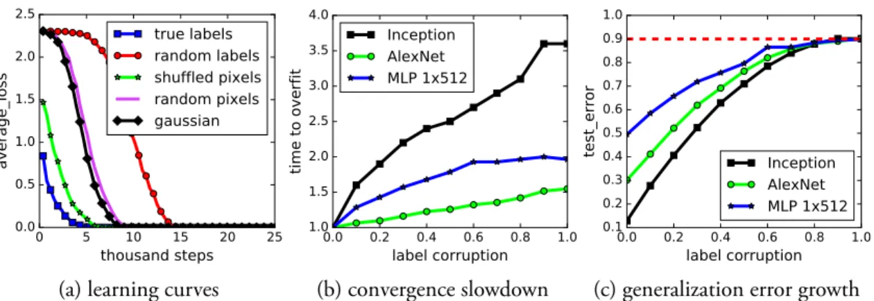
Randomization tests. At the heart of our methodology is a variant of the well-known ran-domization test from non-parametric statistics [Edgington and Onghena,2007]. In a first set of experiments, we train several standard architectures on a copy of the data where the true labels were replaced by random labels. Our central finding can be summarized as:
More precisely, when trained on a completely random labeling of the true data, neural net-works achieve 0 training error. The test error, of course, is no better than random chance as there is no correlation between the training labels and the test labels. In other words, by ran-domizing labels alone we can force the generalization error of a model to jump up considerably without changing the model, its size, hyperparameters, or the optimizer. We establish this fact for several different standard architectures trained on the CIFAR-10 and ImageNet classifica-tion benchmarks. While simple to state, this observaclassifica-tion has profound implicaclassifica-tions from a statistical learning perspective:
1. The effective capacity of neural networks is sufficient for memorizing the entire data set.
2. Even optimization on random labels remains easy. In fact, training time increases only by a small constant factor compared with training on the true labels.
3. Randomizing labels is solely a data transformation, leaving all other properties of the learning problem unchanged.
Extending on this first set of experiments, we also replace the true images by completely random pixels (e.g., Gaussian noise) and observe that convolutional neural networks continue to fit the data with zero training error. This shows that despite their structure, convolutional neural nets can fit random noise. We furthermore vary the amount of randomization, inter-polating smoothly between the case of no noise and complete noise. This leads to a range of intermediate learning problems where there remains some level of signal in the labels. We ob-serve a steady deterioration of the generalization error as we increase the noise level. This shows that neural networks are able to capture the remaining signal in the data, while at the same time fit the noisy part using brute-force.
We discuss in further detail below how these observations rule out all of VC-dimension, Rademacher complexity, and uniform stability as possible explanations for the generalization performance of state-of-the-art neural networks.
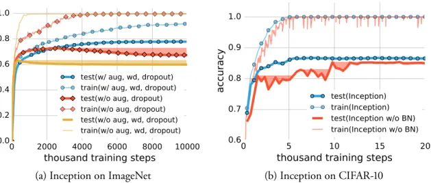
The role of explicit regularization. If the model architecture itself isn’t a sufficient
of regularization, such as weight decay, dropout, and data augmentation, do not adequately explain the generalization error of neural networks. Put differently:
Explicit regularization may improve generalization performance, but is neither necessary nor by itself sufficient for controlling generalization error.
In contrast with classical convex empirical risk minimization, where explicit regularization is necessary to rule out trivial solutions, we found that regularization plays a rather different role in deep learning. It appears to be more of a tuning parameter that often helps improve the final test error of a model, but the absence of all regularization does not necessarily imply poor generalization error. As reported byKrizhevsky et al.[2012], ℓ2-regularization (weight decay) sometimes even helps optimization, illustrating its poorly understood nature in deep learning.
Finite sample expressivity. We complement our empirical observations with a theoretical
construction showing that generically large neural networks can express any labeling of the train-ing data. More formally, we exhibit a very simple two-layer ReLU network with p = 2n + d parameters that can express any labeling of any sample of size n in d dimensions. A previ-ous construction due toLivni et al.[2014] achieved a similar result with far more parameters, namely,O(dn). While our depth 2 network inevitably has large width, we can also come up with a depth k network in which each layer has onlyO(n/k) parameters.
While prior expressivity results focused on what functions neural nets can represent over the entire domain, we focus instead on the expressivity of neural nets with regards to a finite sample. In contrast to existing depth separations [Delalleau and Bengio,2011,Eldan and Shamir,2015,
Telgarsky,2016,Cohen and Shashua,2016] in function space, our result shows that even depth-2networks of linear size can already represent any labeling of the training data.
The role of implicit regularization. While explicit regularizers like dropout and
weight-decay may not be essential for generalization, it is certainly the case that not all models that fit the training data well generalize well. Indeed, in neural networks, we almost always choose our model as the output of running stochastic gradient descent. Appealing to linear models, we analyze how SGD acts as an implicit regularizer. For linear models, SGD always converges to
a solution with small norm. Hence, the algorithm itself is implicitly regularizing the solution. Indeed, we show on small data sets that even Gaussian kernel methods can generalize well with no regularization. Though this doesn’t explain why certain architectures generalize better than other architectures, it does suggest that more investigation is needed to understand exactly what the properties are inherited by models that were trained using SGD.
2.4.2
Related work
Hardt et al.[2016] give an upper bound on the generalization error of a model trained with stochastic gradient descent in terms of the number of steps gradient descent took. Their analysis goes through the notion of uniform stability [Bousquet and Elisseeff, 2002]. As we point out in this work, uniform stability of a learning algorithm is independent of the labeling of the training data. Hence, the concept is not strong enough to distinguish between the models trained on the true labels (small generalization error) and models trained on random labels (high generalization error). This also highlights why the analysis of Hardt et al. [2016] for non-convex optimization was rather pessimistic, allowing only a very few passes over the data. Our results show that even empirically training neural networks is not uniformly stable for many passes over the data. Consequently, a weaker stability notion is necessary to make further progress along this direction.
There has been much work on the representational power of neural networks, starting from universal approximation theorems for multi-layer perceptrons [Gybenko,1989,Mhaskar,1993,
Delalleau and Bengio, 2011, Mhaskar and Poggio, 2016, Eldan and Shamir, 2015, Telgarsky,
2016,Cohen and Shashua,2016]. All of these results are at the population level characterizing which mathematical functions certain families of neural networks can express over the entire domain. We instead study the representational power of neural networks for a finite sample of size n. This leads to a very simple proof that even O(n)-sized two-layer perceptrons have universal finite-sample expressivity.
Bartlett [1998] proved bounds on the fat shattering dimension of multilayer perceptrons with sigmoid activations in terms of the ℓ1-norm of the weights at each node. This important result gives a generalization bound for neural nets that is independent of the network size. However, for RELU networks the ℓ1-norm is no longer informative. This leads to the question
of whether there is a different form of capacity control that bounds generalization error for large neural nets. This question was raised in a thought-provoking work byNeyshabur et al.[2014], who argued through experiments that network size is not the main form of capacity control for neural networks. An analogy to matrix factorization illustrated the importance of implicit regularization.
2.4.3
Effective capacity of neural networks
Our goal is to understand the effective model capacity of feed-forward neural networks. Toward this goal, we choose a methodology inspired by non-parametric randomization tests. Specifi-cally, we take a candidate architecture and train it both on the true data and on a copy of the data in which the true labels were replaced by random labels. In the second case, there is no longer any relationship between the instances and the class labels. As a result, learning is impossible. Intuition suggests that this impossibility should manifest itself clearly during train-ing, e.g., by training not converging or slowing down substantially. To our surprise, several properties of the training process for multiple standard achitectures is largely unaffected by this transformation of the labels. This poses a conceptual challenge. Whatever justification we had for expecting a small generalization error to begin with must no longer apply to the case of random labels.
To gain further insight into this phenomenon, we experiment with different levels of ran-domization exploring the continuum between no label noise and completely corrupted labels. We also try out different randomizations of the inputs (rather than labels), arriving at the same general conclusion.
The experiments are run on two image classification datasets, the CIFAR-10 dataset [Krizhevsky and Hinton,2009] and the ImageNet [Russakovsky et al., 2015] ILSVRC 2012 dataset. We test the Inception V3 [Szegedy et al.,2016] architecture on ImageNet and a smaller version of In-ception, Alexnet [Krizhevsky et al.,2012], and MLPs on CIFAR-10. Please see Subsection2.4.8
in the appendix for more details of the experimental setup.
Fitting random labels and pixels