HAL Id: hal-03022582
https://hal.sorbonne-universite.fr/hal-03022582
Submitted on 24 Nov 2020
HAL is a multi-disciplinary open access
archive for the deposit and dissemination of
sci-entific research documents, whether they are
pub-lished or not. The documents may come from
teaching and research institutions in France or
abroad, or from public or private research centers.
L’archive ouverte pluridisciplinaire HAL, est
destinée au dépôt et à la diffusion de documents
scientifiques de niveau recherche, publiés ou non,
émanant des établissements d’enseignement et de
recherche français ou étrangers, des laboratoires
publics ou privés.
Equilibrium Simulations
Allison Wing, Catherine Stauffer, Tobias Becker, Kevin Reed, Min-Seop Ahn,
Nathan Arnold, Sandrine Bony, Mark Branson, George Bryan, Jean-Pierre
Chaboureau, et al.
To cite this version:
Allison Wing, Catherine Stauffer, Tobias Becker, Kevin Reed, Min-Seop Ahn, et al.. Clouds and
Convective Self-Aggregation in a Multimodel Ensemble of Radiative-Convective Equilibrium
Simula-tions. Journal of Advances in Modeling Earth Systems, American Geophysical Union, 2020, 12 (9),
�10.1029/2020MS002138�. �hal-03022582�
Clouds and Convective Self
‐Aggregation in a Multimodel
Ensemble of Radiative
‐Convective
Equilibrium Simulations
Allison A. Wing1 , Catherine L. Stauffer1 , Tobias Becker2 , Kevin A. Reed3 , Min‐Seop Ahn4 , Nathan P. Arnold5 , Sandrine Bony6 , Mark Branson7 , George H. Bryan8 , Jean‐Pierre Chaboureau9 , Stephan R. De Roode10 , Kulkarni Gayatri11 , Cathy Hohenegger2 , I‐Kuan Hu12, Fredrik Jansson10,13 , Todd R. Jones14 , Marat Khairoutdinov15 , Daehyun Kim4 , Zane K. Martin16 ,
Shuhei Matsugishi17, Brian Medeiros8 , Hiroaki Miura18, Yumin Moon4, Sebastian K. Müller2, Tomoki Ohno19 , Max Popp20 , Thara Prabhakaran11 , David Randall7 ,
Rosimar Rios‐Berrios8 , Nicolas Rochetin2,20 , Romain Roehrig21 , David M. Romps22,23, James H. Ruppert Jr.24 , Masaki Satoh17 , Levi G. Silvers3 , Martin S. Singh25 , Bjorn Stevens2 , Lorenzo Tomassini26 , Chiel C. van Heerwaarden27 ,
Shuguang Wang16 , and Ming Zhao28
1Department of Earth, Ocean and Atmospheric Science, Florida State University, Tallahassee, FL, USA,2Max Planck Institute for Meteorology, Hamburg, Germany,3School of Marine and Atmospheric Sciences, Stony Brook University, Stony Brook, NY, USA,4Department of Atmospheric Sciences, University of Washington, Seattle, WA, USA,5Global Modeling and Assimilation Office, NASA Goddard Space Flight Center, Greenbelt, MD, USA,6Laboratoire de
Météorologie Dynamique (LMD)/IPSL/Sorbonne Université/CNRS, Paris, France,7Department of Atmospheric Science, Colorado State University, Fort Collins, CO, USA,8National Center for Atmospheric Research, Boulder, CO, USA, 9Laboratoire d'Aérologie, Université de Toulouse, CNRS, UPS, Toulouse, France,10Faculty of Civil Engineering and Geosciences, Department of Geoscience and Remote Sensing, Delft University of Technology, Delft, Netherlands,11Indian Institute of Tropical Meteorology, Pune, India,12Rosenstiel School of Marine and Atmospheric Science, University of Miami, Miami, FL, USA,13Centrum Wiskunde and Informatica, Amsterdam, Netherlands,14Department of Meteorology, University of Reading, Reading, UK,15School of Marine and Atmospheric Sciences, and Institute for Advanced Computational Science, Stony Brook University, State University of New York, Stony Brook, NY, USA,16Department of Applied Physics and Applied Mathematics, Columbia University, New York, NY, USA,17Atmosphere and Ocean Research Institute, The University of Tokyo, Kashiwa, Japan,18Department of Earth and Planetary Science, Graduate School of Science, The University of Tokyo, Tokyo, Japan,19Japan Agency for Marine‐Earth Science and Technology, Yokohama, Japan,20Laboratoire de Météorologie Dynamique (LMD)/IPSL/Sorbonne Université/CNRS/École Polytechnique/École Normale Supérieure, Paris, France,21CNRM, Université de Toulouse, Météo‐France, CNRS, Toulouse, France,22Department of Earth and Planetary Science, University of California, Berkeley, CA, USA,23Climate and Ecosystem Sciences Division, Lawrence Berkeley National Laboratory, Berkeley, CA, USA,24Department of Meteorology and Atmospheric Science and Center for Advanced Data Assimilation and Predictability Techniques, Pennsylvania State University, University Park, PA, USA,25School of Earth, Atmosphere, and Environment, Monash University, Clayton, Victoria, Australia,26Met Office, Exeter, UK,27Meteorology and Air Quality Group, Wageningen University, Wageningen, Netherlands,28NOAA/Geophysical Fluid Dynamics Laboratory, Princeton, NJ, USA
Abstract
The Radiative‐Convective Equilibrium Model Intercomparison Project (RCEMIP) is an intercomparison of multiple types of numerical models configured in radiative‐convective equilibrium (RCE). RCE is an idealization of the tropical atmosphere that has long been used to study basic questions in climate science. Here, we employ RCE to investigate the role that clouds and convective activity play in determining cloud feedbacks, climate sensitivity, the state of convective aggregation, and the equilibrium climate. RCEMIP is unique among intercomparisons in its inclusion of a wide range of model types, including atmospheric general circulation models (GCMs), single column models (SCMs), cloud‐resolving models (CRMs), large eddy simulations (LES), and global cloud‐resolving models (GCRMs). The first results are presented from the RCEMIP ensemble of more than 30 models. While there are large differences across the RCEMIP ensemble in the representation of mean profiles of temperature, humidity, and cloudiness, in a majority of models anvil clouds rise, warm, and decrease in area coverage in response to an increase in sea surface temperature (SST). Nearly all models exhibit self‐aggregation in large domains and agree that self‐aggregation acts to dry and warm the troposphere, reduce high cloudiness, and increase©2020. The Authors.
This is an open access article under the terms of the Creative Commons Attribution License, which permits use, distribution and reproduction in any medium, provided the original work is properly cited.
RESEARCH ARTICLE
10.1029/2020MS002138
Special Section:
Using radiative‐convective equilibrium to understand convective organization, clouds, and tropical climate
Key Points:
• Temperature, humidity, and clouds in radiative‐convective equilibrium vary substantially across models • Models agree that self‐aggregation
dries the atmosphere and reduces high cloudiness
• There is no consistency in how self‐aggregation depends on warming Supporting Information: • Supporting Information S1 Correspondence to: A. A. Wing, awing@fsu.edu Citation:
Wing, A. A., Stauffer, C. L., Becker, T., Reed, K. A., Ahn, M.‐S., Arnold, N. P., et al. (2020). Clouds and convective self‐aggregation in a multimodel ensemble of radiative‐convective equilibrium simulations. Journal of
Advances in Modeling Earth Systems,
12, e2020MS002138. https://doi.org/ 10.1029/2020MS002138
Received 10 APR 2020 Accepted 9 JUL 2020
Accepted article online 20 JUL 2020 Corrected 28 OCT 2020
This article was corrected on 28 OCT 2020. See the end of the full text for details.
cooling to space. The degree of self‐aggregation exhibits no clear tendency with warming. There is a wide range of climate sensitivities, but models with parameterized convection tend to have lower climate sensitivities than models with explicit convection. In models with parameterized convection, aggregated simulations have lower climate sensitivities than unaggregated simulations.
Plain Language Summary
This study investigates tropical clouds and climate using results from more than 30 different numerical models set up in a simplified framework. The data set of modelsimulations is unique in that it includes a wide range of model types configured in a consistent manner. We address some of the biggest open questions in climate science, including how cloud properties change with warming and the role that the tendency of clouds to form clusters plays in determining the average climate and how climate changes. While there are large differences in how the different models simulate average temperature, humidity, and cloudiness, in a majority of models, the amount of high clouds decreases as climate warms. Nearly all models simulate a tendency for clouds to cluster together. There is agreement that when the clouds are clustered, the atmosphere is drier with fewer clouds overall. We do notfind a conclusive result for how cloud clustering changes as the climate warms.
1. Introduction
For more than 20 years, coordinated model intercomparisons have been undertaken in which simulations with consistent configurations have been performed with different models to assess whether different mod-els behave similarly and to aid in the understanding of relevant phenomenon. Many of these intercompar-isons have been performed with global climate models, such as the Coupled Model Intercomparison Project (CMIP; Eyring et al., 2016; Meehl et al., 1997, 2000, 2007; Taylor et al., 2012), which was designed to assess the ability of global climate models to robustly simulate important features of the current climate and to evaluate potential future climate changes. The most recent phase (CMIP6; Eyring et al., 2016) includes 21 additional CMIP‐Endorsed Model Intercomparison Projects, which address more targeted scientific ques-tions. Examples include the Cloud Feedback Model Intercomparison Project (CFMIP; Webb et al., 2017), which aims to reduce uncertainty in cloud feedbacks, and the High‐Resolution Model Intercomparison Project (HighResMIP; Haarsma et al., 2016), which investigates the impact of horizontal resolution on regio-nal climate and smaller‐scale phenomena. There are also intercomparisons that exist outside the CMIP infrastructure, some of which employ versions of global models with idealized boundary conditions (e.g., Voigt et al., 2016) or compare specific components of global models, such as the dynamical core (Ullrich et al., 2017). All of the global models that have participated in the aforementioned intercomparisons make use of subgrid‐scale parameterizations, and so another class of intercomparisons that have been influential in the process‐based development of parameterizations is those comparing cloud‐resolving or large eddy simulations of an observational case to single column versions of global models (e.g., Browning et al., 1993; Moeng et al., 1996). Some examples include the CFMIP‐Global Atmospheric System Studies (GASS) Intercomparison of Large eddy models and Single column models (CGILS; Blossey et al., 2013; Zhang et al., 2012, 2013), which compared for thefirst time low cloud feedbacks predicted by models with and without cloud and convective parameterizations, the Global Energy and Water Exchanges project (GEWEX) Atmospheric Boundary Layer Study (GABLS; Bazile et al., 2014; Bosveld et al., 2014; Cuxart et al., 2006; Svensson et al., 2011), which investigated the atmospheric boundary layer, and the European Union Cloud Intercomparison, Process Study, and Evaluation project (EUCLIPSE)‐GASS intercomparison on the stratocumulus to cumulus transition (de Roode et al., 2016; Neggers et al., 2017). More recently, the transi-tion of global modeling to kilometer‐scale resolutransi-tion has motivated the first intercomparison of global cloud‐resolving models (DYAMOND; Stevens et al., 2019).
To date, all model intercomparisons, including those listed above, have been limited to usually one, or at most two, different types of models, rather than incorporating a model hierarchy. This is likely a result of the inherent difficulty in configuring different classes of models in a consistent manner, particularly in com-plex Earth‐like settings. The Radiative‐Convective Equilibrium Model Intercomparison Project (RCEMIP; Wing et al., 2018) overcomes this limitation by employing the idealized framework of radiative‐convective equilibrium (RCE), which is accessible to nearly every conceivable atmospheric model type. To our knowledge, there is no other model intercomparison project that has incorporated such a varied range of model types, including general circulation models (GCMs), single‐column models (SCMs), cloud‐resolving
models (CRMs), large eddy simulations (LES), and global cloud‐resolving models (GCRMs). Thus, RCEMIP presents an unprecedented opportunity to compare models with and without convective parameterizations and in a variety of domain configurations on equal footing.
RCE is the simplest possible description of the climate system, in which radiative cooling of the atmosphere is on average balanced by convective heating. Despite, or perhaps because of its simplicity, there is a long history of modeling RCE in one‐dimensional models (e.g., Manabe & Strickler, 1964; Möller, 1963), two‐ and three‐dimensional CRMs with explicit convection (e.g., Bretherton et al., 2005; Held et al., 1993; Nakajima & Matsuno, 1988; Tompkins & Craig, 1998a), and GCMs with parameterized clouds and convec-tion (e.g., Held et al., 2007; Popke et al., 2013; Reed et al., 2015). RCE remains a popular setting in which to phrase fundamental scientific questions about climate because it eliminates the complexity of imposed het-erogeneities in boundary conditions and forcings (and the resulting dynamical instabilities) but retains the full complexity of moist convective processes and their interaction with radiation and circulation. An initial motivation for the renewed interest in RCE is that insights from more fundamental models might improve more coarse‐grained descriptions of the same phenomena and thus contribute to model development (Popke et al., 2013; Reed & Medeiros, 2016). The importance of using a hierachy of models to understand the climate system, in which understanding is built in simpler contexts that can be connected to more complex systems, has been emphasized by Held (2005, 2014). RCE's status as the simplest representation of the climate system makes it an essential inclusion in such hierarchies (Jeevanjee et al., 2017; Maher et al., 2019). In addition to these formal issues, an intriguing result emerging from cloud‐resolving simulations of RCE is that the inter-action between clouds and circulations can give rise to self‐aggregation of convection, but its importance for climate and the relative role of different driving mechanisms remain unclear and seemingly model depen-dent (Wing, 2019; Wing et al., 2017).
As described in Wing et al. (2018), RCEMIP was motivated by the absence of a common baseline in past simulations of RCE, the accessibility of RCE to a wide range of model types, and the utility of RCE as a fra-mework in which to address some of the biggest open questions in climate science (Bony et al., 2015). With this in mind, RCEMIP was designed to address the following three themes:
1. The robustness of the RCE state across the spectrum of models.
2. The response of clouds to warming and the resulting climate sensitivity in RCE. 3. The dependence of convective self‐aggregation on surface temperature.
While clouds, climate sensitivity, and convective self‐aggregation have all been investigated in RCE before, previous studies have differed in many ways, which has made it difficult to assess whether the diverse results are a real reflection of model uncertainty and lack of understanding or if they are artifacts of the experimen-tal design and/or choice of diagnostics. For example, some modeling studies have found that the spatial extent of tropical anvil clouds decreases with warming (Bony et al., 2016; Cronin & Wing, 2017; Kuang & Hartmann, 2007; Tompkins & Craig, 1999) while others have found an increase (Chen et al., 2016; Ohno & Satoh, 2018; Ohno et al., 2019; Singh & O'Gorman, 2015; Tsushima et al., 2014). Convective self‐ aggregation, which is the spontaneous organization of convection despite homogeneous boundary condi-tions and forcing, has been found to occur across many different models (as reviewed by Wing et al., 2017), but there are some models that do not exhibit spontaneous aggregation under some conditions (Jeevanjee & Romps, 2013), and there is disagreement on the details of the physical mechanisms (Arnold & Randall, 2015; Holloway & Woolnough, 2016; Muller & Bony, 2015; Wing & Emanuel, 2014; Wing et al., 2017). The manner and extent to which self‐aggregation is temperature dependent also remain unresolved, with some studiesfinding that self‐aggregation is favored by high temperatures and others finding no clear temperature dependence, as reviewed by Wing (2019). Several studies have suggested that self‐aggregation, through its effect on humidity and cloudiness, may modulate climate sensitivity (Becker et al., 2017; Coppin & Bony, 2018; Cronin & Wing, 2017; Hohenegger & Stevens, 2016; Mauritsen & Stevens, 2015) and recent estimates from GCMs configured in RCE suggest a climate sensitivity similar to but slightly lower than that of the tropics in comprehensive simulations (Becker & Stevens, 2014; Popke et al., 2013; Silvers et al., 2016). However, the variety of ways in which climate sensitivity in RCE was estimated in these studies, including the type of forcing, the climate perturbation, the background state, and whether the model is uncoupled or coupled to an ocean (usually an idealized slab ocean) at the lower boundary, impedes their interpretation. RCEMIP addresses many of these issues through the specification of a standard protocol.
10.1029/2020MS002138
The objective of this paper is to provide afirst broad overview of the RCEMIP simulations, with a focus on documenting the RCEMIP ensemble and characterizing the RCE state and its robustness across the spec-trum of models. We discuss each of the three above‐mentioned RCEMIP themes and point out notable pat-terns of behavior, such as if models with explicit convection behave differently than models with parameterized convection. However, it is beyond the scope of this paper to provide an explanation for the intermodel spread or the behavior of any one individual model or to investigate detailed physical mechan-isms for changes in response to warming and rigorously test scaling hypotheses. Consistency with prior work is pointed out where appropriate, but detailed investigation of causality is left to future work that can thor-oughly investigate an individual process or model. The results presented in the current paper are a small fraction of the topics that can be explored with the RCEMIP ensemble, so, in addition to serving as a refer-ence for the RCEMIP simulations, we hope that this paper will also stimulate studies into more specific questions and process studies that may require additional experimentation.
While the RCEMIP protocol is described comprehensively in Wing et al. (2018), here we provide details of the configurations of each model participating in RCEMIP and adjustments to the RCEMIP protocol that emerged through the process of its execution (section 2). Section 3 provides a qualitative overview of the ensemble. Section 4 focuses on domain‐ and time‐averaged quantities that characterize the RCE state in the simulations with a surface temperature of 300 K. Self‐aggregation of convection is diagnosed in section 5, including its impact on the mean state. Section 6 describes the response of clouds, self‐aggregation, and the radiative budget to warming by leveraging the suite of simulations performed across three sea surface tem-peratures (SSTs). Conclusions are presented in section 7.
2. RCEMIP Simulations
The RCEMIP protocol is described in Wing et al. (2018); here we briefly review the configuration that is sum-marized in Table 1. A list of the models participating in RCEMIP is provided in Table 2. Text S1 in the supporting information provides additional details of the configuration of each model.
RCEMIP consists of simulations at three different SSTs (SST = 295, 300, and 305 K) in two different domain configurations (RCE_small and RCE_large) for a total of six simulations for each model (Table 1). Models are configured as aquaplanets, with no land or sea ice and a fixed, uniform SST; these are atmosphere‐only simulations with no planetary rotation. The solar insolation is made spatially uniform byfixing the solar zenith angle and solar constant; there is no diurnal or seasonal cycle, and the insolation is everywhere equal to the tropical annual mean (409.6 W m−2). All trace‐gas concentrations other than water vapor are fixed (Wing et al., 2018) and spatially uniform, and there are no aerosol radiative effects, but shortwave and longwave radiative heating rates are calculated interactively from the modeled state using the individual model's radiation scheme. Surface fluxes are calculated interactively from the resolved surface wind speed and air‐sea enthalpy disequilibrium. The RCE_small simulations are initialized from an analytic approximation to the moist tropical sounding of Dunion (2011). In most cases, the RCE_large simulations are initialized from a domain and time average of the equilibrium state in the corresponding RCE_smallsimulation, though there are a few exceptions in which GCMs that do not have a corresponding RCE_small configuration use a different initialization procedure. The initial temperature and moisture sounding is identical at every grid point with zero initial wind; symmetry is broken and convection is generated by applying random, thermal noise in the lowest model layers.
Thefirst class of models that participate in RCEMIP are those with explicit convection, which includes CRMs, GCRMs, and LES (Table 2). CRMs employ a three‐dimensional planar domain with doubly periodic lateral boundary conditions; for RCE_small, the domain is a square of∼100 × ∼100 km2with a horizontal grid spacing of 1 km, while for RCE_large, the domain is an elongated channel of∼6,000 × ∼400 km2with a horizontal grid spacing of 3 km (Table 1). We expect that self‐aggregation will be suppressed in RCE_small and more easily triggered in RCE_large due to the latter's larger domain and coarser resolu-tion (Muller & Bony, 2015; Muller & Held, 2012), though it is unknown if all models exhibit these dependen-cies a priori. The model top is at∼33 km with ∼74 vertical levels (the vertical levels are specified in Wing et al., 2018). Due to numerical and model configuration constraints, each model does not have precisely the same domain size or number of grid points but instead uses values as close as possible to those given above (Text S1). The simulations are run for 100 days. Three models perform GCRM simulations: MPAS,
NICAM, and SAM‐GCRM. To reduce the computational expense of the simulations, MPAS performed global simulations with a reduced Earth radius of RE/8 while NICAM and SAM‐GCRM employ a reduced Earth radius of RE/4. As with the CRMs, the GCRM simulations have grid spacings of∼3–4 km and ∼74 vertical levels and are run for 100 days (Table 1; Text S1).
Table 1
Simulation Configuration
Simulation type Model type Convection Domain size Grid spacing Vertical levels RCE_small CRM Explicit ∼100 × ∼100 km2 1 km ∼74
RCE_small SCM Parameterized Single column N/A as in CMIP6 RCE_large CRM Explicit ∼6,000 × ∼400 km2 3 km ∼74 RCE_large GCRM Explicit Reduced sphere global ∼3‐4 km ∼74 RCE_large GCM Parameterized Global ∼1° as in CMIP6 RCE_large WRF‐GCM Parameterized ∼6000 × ∼400 km2 50 km 48
RCE_small_vert CRM Explicit ∼100 × ∼100 km2 1 km ∼146 RCE_small_les LES Explicit ∼100 × ∼100 km2 200 m ∼146
Table 2
Participating Models
Model abbreviation Model name/version Model type
CM1 Cloud Model 1, cm1r19.6 CRM/LES
DALES Dutch Atmospheric Large‐Eddy Simulation model v4.2 CRM/LES DALES‐damping Dutch Atmospheric Large‐Eddy Simulation model v4.2 CRM
DAM Das Atmosphaerische Modell CRM
FV3 GFDL‐FV3CRM CRM
ICON‐LEM ICOsahedral Nonhydrostatic‐2.3.00, LEM config. CRM/LES ICON‐NWP ICOsahedral Nonhydrostatic‐2.3.00, NWP config. CRM
MESONH Meso‐NH v5.4.1 CRM/LES
MicroHH MicroHH v2.0 CRM/LES
SAM‐CRM System for Atmospheric Modeling 6.11.2 CRM/LES
SCALE SCALE v5.2.5 CRM
UCLA‐CRM UCLA Large‐Eddy Simulation model CRM UKMO‐CASIM UK Met Office Idealized Model v11.0 ‐ CASIM CRM UKMO‐RA1‐T UK Met Office Idealized Model v11.0 ‐ RA1‐T CRM UKMO‐RA1‐T‐hrad UK Met Office Idealized Model v11.0 ‐ RA1‐T CRM UKMO‐RA1‐T‐nocloud UK Met Office Idealized Model v11.0 ‐ RA1‐T CRM WRF‐COL‐CRM Weather Research and Forecasting model v3.5.1 CRM WRF‐CRM Weather Research and Forecasting model v3.9.1 CRM MPAS Model for Prediction Across Scales v6.1 GCRM NICAM Non‐hydrostatic Icosahedral Atmospheric Model v16.3 GCRM SAM‐GCRM System for Atmospheric Modeling v7.3 GCRM CAM5‐GCM Community Atmosphere Model v5 GCM/SCM CAM6‐GCM Community Atmosphere Model v6 GCM/SCM CNRM‐CM6‐1 Atmospheric component of the CNRM Climate Model 6.1 GCM/SCM ECHAM6‐GCM MPI‐M Earth System Model‐Atmosphere component v6.3.04p1 GCM GEOS‐GCM Goddard Earth Observing System model v5.21 GCM/SCM ICON‐GCM ICOsahedral Nonhydrostatic Earth System Model‐Atmosphere component GCM
IPSL‐CM6 IPSL‐CM6A‐LR GCM
SAM0‐UNICON Seoul National University Atmosphere Model v0 GCM SP‐CAM Super‐Parameterized Community Atmosphere Model GCM SPX‐CAM Multi‐instance Super‐Parameterized CAM GCM UKMO‐GA7.1 UK Met Office Unified Model Global Atmosphere v7.1 GCM/SCM WRF‐GCM‐cps0 Weather Research and Forecasting model v3.5.1‐ no conv. param. GCM WRF‐GCM‐cps1 Weather Research and Forecasting model v3.5.1‐ KF GCM WRF‐GCM‐cps2 Weather Research and Forecasting model v3.5.1‐ BMJ GCM WRF‐GCM‐cps3 Weather Research and Forecasting model v3.5.1‐ GF GCM WRF‐GCM‐cps4 Weather Research and Forecasting model v3.5.1‐ SAS GCM WRF‐GCM‐cps6 Weather Research and Forecasting model v3.5.1‐ Tiedtke GCM
10.1029/2020MS002138
Six models perform LES in addition to the CRM simulations (Table 2). These experiments use the ∼100 × ∼100 km2 square domain of the RCE_small setup, but with more vertical levels, smaller horizontal grid spacing, and, in some cases, different parameterizations for subgrid‐scale turbulence. Thefirst set of experiments, RCE_small_vert, performed at each of the three SSTs, are identical to RCE_small but have approxi-mately double the number of vertical levels (Table 1). The specified 146 levels are in Table 3 and feature a stretched grid with 26 levels in the lowest 3 km, 200 m vertical grid spacing from 3 to 22 km, stretched to 500 m at 25 km, and then 500 m between there and the model top of 33 km (note that some models may use slightly different levels due to their unique configurations). The second set of simulations, RCE_small_les, per-formed at each of the three SSTs, has the same vertical levels as RCE_small_vert but use 200 m horizontal grid spacing (Table 1). These simulations are initialized from the mean profiles of the equili-brated RCE_small_vert simulation at the corresponding SST and are run for 50 days.
The second class of models are those that employ parameterized convec-tion, which includes GCMs and SCMs (Table 2). For RCE_large simula-tions, GCMs employ a global spherical domain with horizontal and vertical grids similar to their CMIP6 configuration (Table 1; Text S1). If GCMs perform RCE_small, they do so with the SCM version of the par-ent GCM (see CAM5‐GCM, CAM6‐GCM, CNRM‐CM6‐1, GEOS‐GCM, and UKMO‐GA7.1). The SCM simulations are comparable to the CRM RCE_small simulations because ∼100 km is a typical GCM grid size. The simulations are performed for at least 1,000 days, except for IPSL‐ CM6, which was limited to 630 days.
One exception to the GCM configuration is WRF‐GCM, which employs 50 km horizontal grid spacing and GCM column physics (including a con-vective parameterization) but on the Cartesian geometry used for CRM simulations, rather than the global sphere. This configuration is intended to bridge the gap between the limited area CRM setup and the global GCM setup. Six sets of WRF‐GCM simulations are performed, one with no con-vective parameterization andfive each with a different convective para-meterization (see Text S1). The same version of WRF is also used to perform CRM simulations with 3 km grid spacing and explicit convection (WRF‐COL‐CRM).
With the exception of the RCE_small configuration for models with parameterized convection, which uses one‐dimensional SCMs, all the RCEMIP simulations are three dimensional. Two‐dimensional simula-tions are much more computationally efficient and thus have been used in many past RCE studies of tropical convection (e.g., Islam et al., 1993; Grabowski et al., 1996; Nakajima & Matsuno, 1988; Sui et al., 1994; Randall et al., 1994). Two‐dimensional simulations of RCE have been found to feature self‐aggregation (Brenowitz et al., 2018; Held et al., 1993; Grabowski & Moncrieff, 2001, 2002; Jeevanjee & Romps, 2013; Seidel & Yang, 2020; Stephens et al., 2008; van den Heever et al., 2011; Yang, 2018a, 2018b). However, RCEMIP focuses on three‐dimensional simulations in order to compare CRMs and global models and to be inclusive in the models that may participate (many models cannot be easily configured in two dimen-sions). The dimensionality of the simulation is another factor that could affect the simulated RCE state, which could be considered in a future extension of RCEMIP using a subset of the models.
The hierarchy of models included in RCEMIP offers an opportunity to assess the robustness of the simu-lated RCE state. In addition to examining the entire ensemble and subsetting by model type (i.e., explicit Table 3
Vertical Levels for RCE_small_vert and RCE_small_les Level (m) Height (m) Level Height (m) Level Height (m) Level Height 1 20 47 7,200 93 16,400 139 29,500 2 60 48 7,400 94 16,600 140 30,000 3 107 49 7,600 95 16,800 141 30,500 4 160 50 7,800 96 17,000 142 31,000 5 220 51 8,000 97 17,200 143 31,500 6 286 52 8,200 98 17,400 144 32,000 7 359 53 8,400 99 17,600 145 32,500 8 439 54 8,600 100 17,800 146 33,000 9 525 55 8,800 101 18,000 10 618 56 9,000 102 18,200 11 717 57 9,200 103 18,400 12 823 58 9,400 104 18,600 13 936 59 9,600 105 18,800 14 1,055 60 9,800 106 19,000 15 1,181 61 10,000 107 19,200 16 1,314 62 10,200 108 19,400 17 1,453 63 10,400 109 19,600 18 1,599 64 10,600 110 19,800 19 1,751 65 10,800 111 20,000 20 1,910 66 11,000 112 20,200 21 2,076 67 11,200 113 20,400 22 2,248 68 11,400 114 20,600 23 2,427 69 11,600 115 20,800 24 2,612 70 11,800 116 21,000 25 2,804 71 12,000 117 21,200 26 3,000 72 12,200 118 21,400 27 3,200 73 12,400 119 21,600 28 3,400 74 12,600 120 21,800 29 3,600 75 12,800 121 22,000 30 3,800 76 13,000 122 22,220 31 4,000 77 13,200 123 22,463 32 4,200 78 13,400 124 22,730 33 4,400 79 13,600 125 23,023 34 4,600 80 13,800 126 23,347 35 4,800 81 14,000 127 23,703 36 5,000 82 14,200 128 24,096 37 5,200 83 14,400 129 24,527 38 5,400 84 14,600 130 25,000 39 5,600 85 14,800 131 25,500 40 5,800 86 15,000 132 26,000 41 6,000 87 15,200 133 26,500 42 6,200 88 15,400 134 27,000 43 6,400 89 15,600 135 27,500 44 6,600 90 15,800 136 28,000 45 6,800 91 16,000 137 28,500 46 7,000 92 16,200 138 29,000
vs. parameterized) and domain configuration (RCE_small vs. RCE_large), there is the opportunity for more targeted comparisons. For example, the set of WRF‐GCM simulations allows the impact of different deep convective parameterizations to be analyzed. Comparing CAM5‐GCM, CAM6‐GCM, SAM0‐ UNICON, SP‐CAM, and SPX‐CAM can reveal how the representation of convection affects the RCE state across the same parent model. CAM5‐GCM and CAM6‐GCM differ in most of their physics packages but have the same deep convective parameterization with similar parameter settings. SAM is used to perform GCRM, CRM, and LES experiments, which allows for the same modeling system to be examined across different geometries and resolutions. Similarly, ICON is used to perform global simulations in its GCM configuration, CRM configurations using two different sets of physics packages, and an LES configuration. UKMO‐CASIM and UKMO‐RA1‐T differ in the microphysics scheme used, while UKMO‐RA1‐T and UKMO‐RA1‐T‐nocloud differ in that the cloud scheme is disabled in the latter. DALES‐damping is identical to DALES except weak damping of the horizontal‐mean horizontal winds to zero is applied (to compensate for the generation of horizontal layers of high winds in the stratosphere due to weak turbulence production). SP‐CAM and SPX‐CAM differ only in how surface enthalpy fluxes are calculated (i.e., on the parent GCM grid or superparameterized by the embedded CRMs). These types of comparisons are useful for determining possible causes of intermodel spread and will be the focus of future studies with the RCEMIP simulations.
3. Overview of Simulations
First, we provide a general overview of the simulations by examining the hourly averaged outgoing longwave radiation (OLR) in the RCE_small300, RCE_large300, RCE_small_vert300, and Figure 1. Time series of domain‐mean outgoing longwave radiation (OLR; W m−2) in the RCE_small300 (left column) and RCE_large300 simulations (right column). The top row shows GCM simulations with parameterized convection, with the single‐column version of the model in (a) and the global model in (b). The middle row shows simulations with explicit convection (c, d), including CRM, LES, and GCRM simulations. The bottom row shows the
WRF‐GCM simulations with 50 km resolution and parameterized convection. The black vertical line to the left of each plot is a 25 W m−2 scale bar, but the absolute values of OLR and distance between the curves has no meaning here, as the curves are offset for visual clarity according to OLR +⟨OLR⟩ + i*x x, where ⟨ ⟩ is the ensemble mean, i is the model index (according to alphabetical order), and xx = 2 for RCE_large and xx = 10 for RCE_small.
10.1029/2020MS002138
RCE_small_les300 simulations. The evolution to RCE takes many tens of days (Tompkins & Craig, 1998b; Cronin & Emanuel, 2013), as shown by the domain‐mean OLR time series in Figure 1. The temporal evolution is similar in all models and emphasizes that RCE is a state of stationarity; that is, there is temporal variability but the statistics are invariant to time. The RCE_small simulations (Figures 1a, 1c, and 1e), especially the single‐column simulations in Figure 1a, have more temporal variability than their RCE_large counterparts (Figures 1b, 1d, and 1f). Based on Figure 1, we compute temporal averages to represent the RCE state (section 4) by averaging over time and neglecting thefirst 75 days of simulation (except for RCE_small_les, for which the average is taken over Days 25–50). To examine the distribution of convection after equilibrium is reached, we examine the spatial structure of OLR at Day 80 (Day 50 for RCE_small_les). Equivalent figures for precipitable water (PW) and animations of OLR and PW are included in the supporting information (Figures S1–S5).
Figure 2 shows OLR at Day 80 in the RCE_small300 simulation for all the CRMs. The cloud distribution, as indicated by the white color shading representing cold cloud tops, varies across models. We note that DALES and DALES‐damping have larger values of OLR because the radiative properties of ice clouds were erroneously configured; the grid‐box cloud fraction in the radiation scheme was set to one in the presence of liquid clouds but not ice clouds. If this is corrected, the OLR distribution looks more realistic (see the RCE_small_vert300 simulation for DALES‐damping‐rad in Figure 3). While the RCE state is affected by this error, the sensitivity to SST is similar. The OLR and PW snapshots (Figure S1) and animations indi-cate that, in all models except UKMO‐RA1‐T, convection is quasi‐randomly distributed in space and time with nearly spatially uniform PW, reflecting unaggregated convection in the small domain. While ICON‐NWP appears slightly aggregated toward the beginning of the simulations at 300 and 305 K, UKMO‐RA1‐T is the only model that exhibits consistent convective aggregation in RCE_small. This sug-gests that the minimum domain size required for self‐aggregation (Muller & Held, 2012) is model dependent, since self‐aggregation was not expected in the RCE_small ∼100 × ∼100 km2
domain. Since part of the objective of the RCE_small simulations is to provide an unaggregated control to compare to, an additional set of RCE_small simulations was performed with UKMO‐RA1‐T in which the radiative heating rates were spatially homogenized (UKMO‐RA1‐T‐hrad). This prevents aggregation, and it is these simulations from which the UKMO‐RA1‐T RCE_large simulations are initialized. Figure 3 shows OLR in the RCE_small300, RCE_small_vert300, and RCE_small_les300 simulations for the six models that performed them (CM1, DALES, ICON‐LEM, MESONH, MicroHH, and SAM). All simulations are unaggre-gated, and the LES simulations havefiner spatial structures, but otherwise, there are no obvious differences compared to the RCE_smallsimulations (see also Figure S2 and animations).
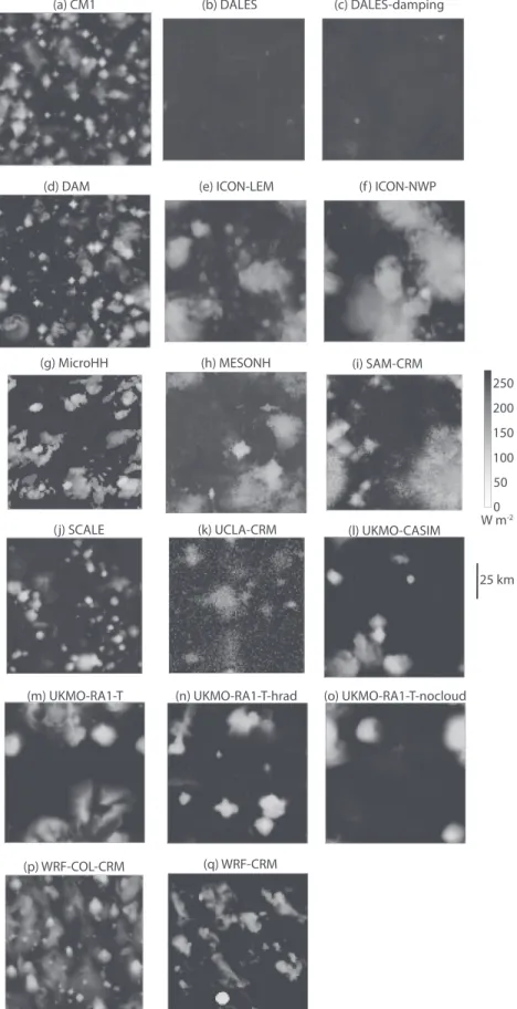
Figure 4 shows OLR at Day 80 in the RCE_large300 simulation for all the CRMs. Except for WRF‐CRM, the condensatefield simulated by all of the models shows evidence of large‐scale clustering or aggregation. The way in which the condensate is clustered, however, differs. Differences are evident in the number of aggregated regions, their spatial scale, and their orientation. This clustering is also evident in the distribution of PW, which varies in association with the condensatefield (Figure S3), in contrast to the RCE_small simulations (Figures S1 and S2). Animations and y‐averaged Hovmöller diagrams reveal a rich spectrum of variability, including the growth and decay of individual convective cells within the aggregated envelope, propagation of gravity waves, sloshing of the convection along the x direction, mergers and splitting of convective bands, and expansion and contraction of dry and clear air regions (Figure S6). Some models appear visually to be more aggregated than others (e.g., UKMO‐RA‐1‐T appears more aggregated than UKMO‐CASIM); the degree of aggregation will be quantified in section 5.
Figure 5 shows OLR in the RCE_large300 simulation at Day 80 for all the global model (GCM and GCRM) simulations. Each GCRM is shown to scale based on its reduced Earth radius, along with an additional zoomed‐in view. The supporting information contains a figure that shows OLR in a subset of the global domains that is approximately the size of the CRM domain, for comparison (Figure S9). The global simula-tions all appear aggregated to some extent, but there is diversity in the spatial structure of convection; some simulations have one or two hemisphere‐scale aggregated regions (e.g., NICAM and CAM5), some have quasi‐regularly spaced aggregated clusters (e.g., UKMO‐GA7.1, ECHAM, ICON‐GCM, and IPSL‐CM6), some have convection organized along irregular lines (e.g., CNRM‐CM6‐1), and others seem only partially aggregated, with only a few dry, clear patches amidst more uniform convection (e.g., CAM6‐GCM, GEOS‐
Figure 2. Hourly‐averaged outgoing longwave radiation (W m−2) at Day 80 of the RCE_small300 simulation for all cloud‐resolving models. Each panel displays a different model and the size of each panel represents the domain size, which varies slightly across models.
10.1029/2020MS002138
GCM, and MPAS). These differences are also reflected in the distribution of PW (Figure S4). Animations indicate that the convective patterns are approximately stationary in most of the models, with the cloudfield as represented by OLR varying more rapidly than the PW field (see also Figure S7). SPX‐CAM, SAM0‐UNICON, and CAM6‐GCM have more tem-poral variability in the convective regions than other models, and the con-vective clusters in MPAS seem to propagate around a large central dry patch. The degree of aggregation is quantified in section 5, and discussion of the qualitative sensitivity of the patterns of aggregation and their temporal variability to SST is provided in section 6.2.
Figure 6 shows OLR at Day 80 in the RCE_large300 simulation in the set of WRF simulations that include a CRM configuration (WRF‐COL‐ CRM) and a GCM‐like configuration in Cartesian geometry (WRF‐ GCM). In addition to the obvious difference in fine‐scale structures between the 3 and 50 km resolutions, for the same parent model, the GCM versions seem more aggregated than the CRM version (WRF‐ COL‐CRM). Among the different WRF‐GCM versions, there are no obvious differences in the scale or degree of aggregation (see also PW in Figure S5). We note that WRF‐COL‐CRM becomes slightly more aggre-gated later in the simulation with more persistent dry regions (Movie S27). The only model in the overall RCEMIP ensemble that does not aggregate, WRF‐CRM, is a newer version of WRF than WRF‐COL‐CRM that employs different radiation and microphysics schemes.
In summary, while the spatial patterns of convection are diverse, all but one (UKMO‐RA1‐T) of the RCE_small simulations appear unaggre-gated, and all but one (WRF‐CRM) of the RCE_large simulations appear aggregated, to varying extents. The emergence of aggregation is indepen-dent of the representation of convection (i.e., explicit vs. parameterized). The next section will analyze whether the diverse spatial patterns lead to similar or different domain‐mean characteristics of the RCE state.
4. The RCE State
In this section, we characterize the RCE state across the RCEMIP ensem-ble by considering domain‐ and time‐average quantities, neglecting the first 75 days. We focus on temperature, humidity, clouds, and quantities related to the mean top‐of‐atmosphere energy budget. We discuss the results in RCE_small and RCE_large separately; the difference between pairs of RCE_small and RCE_large simulations is discussed in section 5. We focus on the simulations at 300 K, as representative of the current tropical climate. Results for the simulations at 295 and 305 K can be found in the supporting information (Figures S11–S18).
4.1. Temperature
The domain‐ and time‐averaged temperature profiles are shown in Figure 7, in which thefirst column shows the ensemble mean and spread across all models while the other columns display the temperature anom-aly in each subgroup of models as an anomanom-aly from the ensemble mean of that subgroup. The intermodel spread across all models is similar in the RCE_small and RCE_large simulations, considering the ensemble range and the interquartile range (Figures 7a and 7e). We expect that the troposphere in RCE should evolve toward a roughly moist adiabatic temperature profile. While the average tropospheric lapse rate (averaged between the surface and the radiative tropopause) in the RCE_small simulations is 7.5 K km−1(Figure 11), the temperature profiles Figure 3. Hourly averaged outgoing longwave radiation (W m−2) at Day 80
of the RCE_small300 (a, d, g, j, m, p, s) and RCE_small_vert300 (b, e, h, k, n, q, t) simulations and Day 50 of the RCE_small_les300 (c, f, l, o, r, u) simulations for CM1, DALES, DALES‐damping, ICON_LEM, MESONH, MicroHH, and SAM. The size of each panel represents the domain size, which varies slightly across models. DALES and
DALES‐damping have larger values of OLR because the radiative properties of ice clouds were erroneously configured. DALES‐damping‐rad is a corrected version, shown for reference (note that it is the
RCE_small_vert300 simulation that is shown in panel (i) despite it being in the column with LES simulations).
are systematically several degrees cooler than a moist adiabatic profile (not shown). This is consistent with theory that indicates that tropical temperature profiles are set by dilute moist adiabats in which entrainment systematically reduces cloud updraft moist static energy (Seeley & Romps, 2015; Singh & O'Gorman, 2013). The amount of dilution depends on entrainment rate and precipitation efficiency (Romps, 2016), which may explain the spread in temperature profiles across the RCEMIP simulations. In fact, preliminary analysis suggests that there is a larger deviation from a moist adiabat (more instability) in simulations that are on average moister in the midtroposphere (not shown). An initial calculation indicates that this is qualitatively consistent with expectations from the simple plume model of Romps (2016) in which both Figure 4. Hourly averaged outgoing longwave radiation (W m−2) at Day 80 of the RCE_large300 simulation for all cloud‐resolving models. Each panel displays a different model and the size of each panel represents the domain size, which varies slightly across models. Note that FV3 is missing from thefigure because outgoing longwave radiation was only reported as daily averages.
10.1029/2020MS002138
instability and relative humidity depend on entrainment (see also Romps, 2014; Singh et al., 2019), though this relationship could be complicated by changes in precipitation efficiency across models. The cold point occurs at different heights and at different temperatures across the models but, in the RCE_small300 simulations, is on average 193 K and occurs at an average height of 15.7 km (thefirst and third quartiles are 190.4 and 195.3 K for the temperature and 14.8 and 16.2 km for the height). The radiative tropopause, defined as the first level at which the radiative cooling rate intersects zero, is on average below the cold point, with an average temperature of 205 K (interquartile range of 9.5 K) and an average height of 12.7 km (interquartile range of 1.3 km). The average cold point in RCE_large300 is 197 K at an average height of 16.2 km, and the average radiative tropopause is 205 K at an average height of 15.3 km. While the temperature profile has the same general shape in all models, when considering the temperature anomalies from the ensemble mean, the range in temperatures at a given height can be up to 10 K (Figure 7). UCLA_CRM is notably warmer in the troposphere than the other simulations in both RCE_small and RCE_large (see yellow line to the right of the ensemble of profiles in Figures 7c and 7g). There are also large temperature differences in the lower stratosphere (∼17–20 km), which is somewhat surprising given that the RCEMIP protocol enforces the same trace gas profiles and insolation. Across all simulations, including all SSTs, the average difference between the temperature at the lowest model level and the SST is−2.4 K, though some of the spread (the interquartile range is 1.0 K) is due to the lowest model level being placed at different heights in different models. This air‐sea temperature differ-ence is influenced by the surface sensible heat flux, which is on average 9.4 W m−2in RCE_small300 (Table A1) and 11.2 W m−2in RCE_large300 (Table A2). For those models that report 2 m air tempera-ture, the difference between that and SST is on average−1.7 K, with an interquartile range across models of 0.8 K. The differences reflect differences in boundary layer and surface schemes, including how 2 m air temperatures are estimated.
Figure 5. Hourly averaged outgoing longwave radiation (W m−2) at Day 80 of the RCE_large300 simulation for all global models (except for IPSL‐CM6, which reported daily averaged output). All models shown are GCMs with parameterized convection (panels a–k) except MPAS, NICAM, and SAM (panels l–n), which are global cloud‐resolving models that employ reduced Earth radius of RE/8, RE/4, and RE/4, respectively, and are shown to scale and, in the box,
4.2. Relative Humidity
Relative humidity is calculated based on each model's formulation for saturation over water and ice. Thus, different formulations may be used in different models, but each formulation is consistent with how that model's clouds respond to and regulate relative humidity. Several models inadvertently reported relative humidity with respect to saturation over water at all temperatures. To ensure a representative comparison, we corrected these calculations to relative humidity with respect to saturation over ice at temperatures below freezing using the Wagner and Pruß (2002) and Wagner et al. (2011) formulations. There is a large spread in simulated relative humidity across the RCEMIP ensemble. In the RCE_small simulations, relative humid-ities in the midtroposphere vary between∼25% and ∼90% (Figure 8a), with an average minimum relative humidity between 2 and 10 km of∼61%. Relative humidity near the surface varies from ∼60% to more than ∼80% with an average of ∼73%, but this does not explain the spread in the free troposphere (i.e., if the rela-tive humidity profiles are shifted such that all models start from the same relative humidity value at the low-est model level, the intermodel spread in the free troposphere is actually increased). The large spread in simulated relative humidity may be a result of its control by detrainment (Romps, 2014; Singh et al., 2019), and/or precipitation efficiency and downdrafts (Emanuel, 2019), processes that are likely represented differently across the RCEMIP ensemble. Many of the models are near saturation or supersaturated with respect to ice near the tropopause; this behavior is expected. The LES models also exhibit a large spread in relative humidity in the free troposphere (Figure 8d), but it is smaller than the spread across the same six models in RCE_small300. Half of the LES models have a moister midtroposphere than their RCE_small300 counterparts while half have a drier midtroposphere; the average magnitude of the differ-ence is 4.4.
While there is still a large spread across the models in the RCE_large simulations, there is a more consis-tent shape to the relative humidity profile with a pronounced mid‐level minimum in all models and overall better model agreement (smaller standard deviation and interquartile range, relative to the mean values) Figure 6. Hourly averaged outgoing longwave radiation (W m−2) at Day 80 of the RCE_large300 simulation for all versions of WRF 3.5.1. Panel (a) displays the same WRF‐COL‐CRM configuration as in Figure 4l. The other panels (b–h) show WRF‐GCM in the Cartesian RCE_large300 configuration but with 50 km grid spacing and convective parameterizations.
10.1029/2020MS002138
than in RCE_small (Figure 8e). The models with parameterized convection are in closer agreement than the CRM and GCRM simulations (cf. Figures 8f, and 8g and 8h). ICON_GCM (Figure 8f) is an outlier that is unusually dry in the boundary layer compared to the other models; this is also found in realistic AMIP‐style simulations with ICON and is suspected to be a bug. IPSL‐CM6 (Figure 8f) is also an outlier with generally lower relative humidity. The spread across models in RCE_large is not correlated with the spread across those same models in RCE_small, suggesting that the spread in RCE_large may reflect differences in aggregation moreso than differences in the baseline RCE state.
4.3. Clouds
As with relative humidity, the RCEMIP ensemble exhibits large variability in cloud fraction profiles in the RCE_small simulations (Figures 9a–9d; Table S2), with the peak high (“anvil”) cloud fraction varying an order of magnitude from a low value of∼0.08 in UCLA‐CRM to 1.0 in several of versions of the UKMO Figure 7. Horizontal‐mean temperature profile, averaged in time excluding the first 75 days of simulation of the RCE_small (top row: a–d) and RCE_large
(bottom row: e–h) simulations at 300 K. The first column (a, e) includes all models that performed each type of simulation, where the black line is the ensemble mean, the blue shading shows the range across all models, and the orange lines indicate the interquartile range (IQR). The other columns display the temperature anomaly in each subgroup of models as an anomaly from the ensemble mean of that subgroup, for models with parameterized convection (second column: b, f), CRMs (third column: c, g), models that performed RCE_small_vert (dashed) and RCE_small_les (solid) simulations (panel d; RCE_small_les simulations are averaged over Days 25–50), and GCRMs (panel h).
cloud‐resolving model. A cloud fraction of 1.0 at a particular model level indicates that the entire domain is covered in cloud at that level. In this study, a cloud is defined according to a threshold value of cloud condensate (10−5kg kg−1or 1% of the saturation mixing ratio over water, whichever is smaller) or the output of a cloud scheme (if utilized by a given model). The ICON_LEM simulations also exhibit high cloud fractions very close to 1.0, which stems from clouds that are very optically thin (due to the settings in the microphysics scheme, in which the threshold value for self‐collection is set at 10−6for ice and there is a small sedimentation velocity of ice particles). If an alternate threshold for identifying a cloud is used (e.g., cloud condensate must be larger than 5 × 10⁻⁷kg kg−1), the ICON_LEM cloud fractions are more in line with the other models. In addition to simulating very different amounts of high cloud, there is also a large spread in the height at which the anvil cloud peak occurs (∼9–17 km; Table S4). The intermodel spread in cloud fraction does not collapse when plotted against temperature as a vertical axis, indicating that the models have anvil cloud peaks at different heights because they form them at different Figure 8. Horizontal‐mean relative humidity profile, averaged in time excluding the first 75 days of simulation of the RCE_small (top row a–d) and RCE_large
(bottom row: e–h) simulations at 300 K. The first column (a, e) includes all models that performed each type of simulation, where the black line is the ensemble mean, the blue shading shows the range across all models, and the orange lines indicate the interquartile range (IQR). The other columns display each subgroup of models: models with parameterized convection (second column: b, f), CRMs (third column: c, g), models that performed RCE_small_vert (dashed) and RCE_small_les (solid) simulations (panel d; RCE_small_les simulations are averaged over Days 25–50), and GCRMs (panel h).
10.1029/2020MS002138
temperatures (the interquartile range of anvil cloud temperature is 11.9 K; Table S3). With the exception of CNRM‐CM6‐1, CAM5, and CAM6 (the single‐column versions of GCMs with parameterized convection), all models have very small amounts of mid‐level cloud (∼3–8 km). There is also variability in the amount of low cloud, though generally less variability in the models with explicit convection (Figures 9c and 9d). However, it should be noted that because of the absence of strong subsiding motions, which in nature are generally forced by horizontal heterogeneities in surface boundary conditions, the RCE setup is not favorable to certain tropical low‐cloud regimes such as stratocumulus. MESONH is an outlier among the CRMs, with approximately twice the amount of low cloud than the other models (Figure 9c). The low cloud amount exhibits some sensitivity to resolution, though not always consistently across models (compare curves in Figures 9c and 9d). For the six models that performed RCE_small, RCE_small_vert, and RCE_small_les simulations, low cloud amount increases with an increasing number of vertical levels in ICON_LEM and DALES, decreases in DALES‐damping, and has no change in the other models. Low Figure 9. Domain‐wide cloud fraction profile, averaged in time excluding the first 75 days of simulation of the RCE_small (top row: a–d) and RCE_large
(bottom row: e–h) simulations at 300 K. The first column (a, e) includes all models that performed each type of simulation, where the black line is the ensemble mean, the blue shading shows the range across all models, and the orange lines indicate the interquartile range (IQR). The other columns display each subgroup of models: models with parameterized convection (second column: b, f), CRMs (third column: c, g), models that performed RCE_small_vert (dashed) and RCE_small_les (solid) simulations (panel d; RCE_small_les simulations are averaged over Days 25–50), and GCRMs (panel h).
cloud amount decreases with decreasing horizontal grid spacing in all models except CM1 and MicroHH, for which there is no change.
There is also substantial spread in cloud fraction profiles in the RCE_large simulations (Figures 9e–9h; Table S5), but the high cloud fraction spans a narrower range than in the RCE_small simulations. UCLA‐CRM has notably fewer high clouds than the other CRMs (Figure 9g), and IPSL‐CM6 stands out as an outlier with few high clouds compared to the other models with parameterized convection (Figure 9f). If WRF‐GCM is excluded, there is a suggestion that models with parameterized convection (Figure 9f) have better agreement of anvil cloud amount and exhibit cloudiness that is more uniform throughout the column than the CRMs (Figure 9g). CRMs have more notable anvil and low cloud peaks, consistent with CRMs having fewer mid‐level clouds. WRF‐GCM‐cps0 and WRF‐GCM‐cps3 are outliers that have much higher low cloud fraction than other models with parameterized convection (Figure 9f). In general, there are Figure 10. Horizontal‐mean total cloud water condensate profile, averaged in time excluding the first 75 days of simulation of the RCE_small (top row: a–d) and
RCE_large (bottom row: e–h) simulations at 300 K. The first column (a, e) includes all models that performed each type of simulation, where the black line is the ensemble mean, the blue shading shows the range across all models, and the orange lines indicate the interquartile range (IQR). The other columns display each subgroup of models: models with parameterized convection (second column: b, f), CRMs (third column: c, g), models that performed
RCE_small_vert (dashed) and RCE_small_les (solid) simulations (panel d; RCE_small_les simulations are averaged over Days 25–50), and GCRMs (panel h).
10.1029/2020MS002138
fewer high clouds and more mid‐level clouds in the RCE_large simulations than in the RCE_small simu-lations (Figure 9e cf. Figure 9a).
Cloud fraction depends sensitively on the semiarbitrary threshold used to identify clouds. Therefore, we also examine the horizontal‐mean profiles of total cloud water condensate, which is primarily liquid at low levels and ice at high levels (Figure 10). Consistent with the spread in cloud fraction profiles (Figure 9a), the total cloud water profiles in the RCE_small simulations (Figure 10a) exhibit widely varying amounts of cloud water (by an order of magnitude or more) and differ both in the amount of upper level cloud condensate and the height at which the anvil cloud condensate peak occurs (Figures 10b–10d). The total cloud water profiles vary smoothly with height in the CRM RCE_small simulations (Figure 10c). Among the models with explicit convection (Figures 10c and 10d), the models differ in whether the maximum of the cloud water profile occurs at low altitudes or at high altitudes. For example, the maximum of the cloud water profile of the UKMO family of models is in the upper troposphere whereas the maximum of the cloud water profile for UCLA‐CRM, MPAS, and DAM is in the lower troposphere. Some models, like ICON‐LEM, SAM‐CRM, and WRF‐COL‐CRM, have similar peaks of cloud water in the upper and lower troposphere (Figure 10c). Finer grid spacing does not reduce the spread; among models that performed both CRM and LES simulations, the LES simulations differ as much as their counterparts at coarser resolution (Figure 10d).
The total cloud water profiles appear to have a wider spread in the RCE_large simulations (Figure 10e), with more disagreement in the amount of cloud water than in the RCE_small simulations, but this impres-sion may be a result of the behavior of individual models (i.e., UKMO family in Figure 10g). Models with parameterized convection place their cloud water peaks at very different heights and many models lack a distinct upper level peak (Figure 10f).
The differences in simulated cloudiness in the RCE_small simulations reflect fundamental differences in how the different models handle clouds and in the equilibrium state that each model converges to. The dif-ferences in simulated cloudiness in the RCE_large simulations reflect these difdif-ferences as well as differ-ences in the degree of aggregation simulated by each model and differdiffer-ences in how each model represents the response of cloudiness to self‐aggregation. This will be explored further in later sections.
4.4. Energy Budget and Hydrological Cycle
Appendix A1 provides a summary of domain‐average statistics in each of the simulations at 300 K, including variables related to the energy budget and hydrological cycle. The intermodel spread in a subset of those vari-ables is summarized in Figure 11, which includes domain‐average precipitation rate, net radiation at the top of atmosphere (RTOA), condensed water path, PW, and tropospheric lapse rate. RTOAis calculated as the dif-ference between the net absorbed solar radiation at the top of the atmosphere and the OLR (ASRTOA−OLR). RTOAis positive, representing a net downward radiativeflux, or a net energy gain for the climate system. The condensed water path is calculated as the sum of the cloud ice water path and the cloud liquid water path. The tropospheric lapse rate is calculated as dT/dz averaged over the troposphere, where the top of the troposphere is defined as the height at which the radiative cooling rate first intersects zero.
There are several outliers indicated in Figure 11, defined as points beyond 1.5 times the interquartile range. For precipitation, DALES (4.8 mm day−1) and DALES‐damping (4.6 mm day−1) are outliers from RCE_small300; DALES (5.5 mm day−1), DALES‐damping (4.7 mm day−1), and MicroHH (4.5 mm day−1) are outliers from RCE_small_vert300; and DALES (5.5 mm day−1) is an outlier from RCE_small_les300 (Figure 11a). ICON‐NWP‐CRM (2.2 mm day−1) is the outlier for precipitation in the large simulation. For RTOA, CNRM‐CM6‐1 (58.88 W m−2), WRF‐CRM (57.70 W m−2), and WRF‐ GCM‐cps3 (35.68 W m−2) are the outliers in the small simulation in Figure 11b; WRF‐GCM‐cps3 (12.00 W m−2) is the outlier in the large domain simulation. For lapse rate, WRF‐GCM‐cps2 (−6.08 K km−1), WRF‐GCM‐cps4 (−6.28 K km−1), and WRF‐GCM‐cps6 (−6.21 K km−1) are the outliers in the small simulation (Figure 11e). Overall, there are more outliers in Figures 11a–11e in the RCE_small simulations, contributed by the single‐column versions of models with parameterized con-vection, the very small WRF‐GCM domain, and configurations of DALES and MicroHH. It is notable that all lapse rate outliers are contributed from WRF‐GCM.
There is substantial intermodel spread in all quantities, but tropospheric lapse rate exhibits the best agree-ment, as measured by the interquartile range relative to the mean value (Figure 11e). For some variables
(i.e., net radiation and lapse rate), the spread in the RCE_large simulations is larger than that in the RCE_small simulations, but for other variables the spread is larger in RCE_small or similar between the two configurations. It is therefore difficult to determine whether the intermodel spread in the representation of the RCE state is due to differing degrees of aggregation or to more fundamental differences in model physics and numerics. Furthermore, there is no consistency in whether the intermodel spread is larger in models with explicit or parameterized convection; it is larger in models with explicit convection for precipitation, condensed water path, and PW, but larger in models with parameterized convection for net radiation and lapse rate (Figures 11f–11j).
5. Self‐Aggregation
5.1. Degree of Self‐AggregationThere is no single agreed upon quantitative measure of the degree of aggregation (Wing, 2019); therefore, here we quantify the degree of aggregation using three different metrics: the organization index (Iorg; Tompkins & Semie, 2017), subsidence fraction (fsub; Coppin & Bony, 2015), and the spatial variance of col-umn relative humidity (σ2
CRHWing & Cronin, 2016). An alternate metric, the spatial variance of PW scaled by its mean value, is presented in the supporting information (Figures S24 and S25). Iorgis a clustering metric that compares the nearest neighbor distribution of deep convective entities to that of a random distribution. Figure 11. Box and whiskers plots of domain‐average quantities, averaged in time excluding the first 75 days of the RCE_small300 and RCE_large300
simulations. RCE_small_vert300 and RCE_small_les300 simulations are included in the“Small” statistics. The top row (panels a–e) includes all models in the statistics while the bottom row (panels f–j) splits the models into those with explicit (“SE” and “LE”) and parameterized convection (“SP” and “LP”),
where the“S” and “L” indicate small and large simulations, respectively. The variables shown are precipitation rate (mm day−1; panels a and f), net radiation at the top of atmosphere (RTOA; W m−2, downward defined as positive; panels b and g), condensed water path (CWP; mm; panels c and h),
precipitable water (PW; kg m−2; panels d and i), and the tropospheric lapse rate (K km−1; panels e and j). The asterisk indicates the multimodel mean, the horizontal line the median, the shaded region the interquartile range, and the circles the outliers. The whiskers are defined as 1.5 times the interquartile range; this does not extend beyond the range of the data.
10.1029/2020MS002138
fsubis the area fraction of the domain where the daily‐average large‐scale vertical velocity at 500 hPa is directed downward. Vertical velocity is first averaged in time over a day and in space over ∼100 × ∼100 km2blocks. Column relative humidity (CRH) is defined as the ratio of PW to saturated PW (mass
weighted vertical integrals of specific humidity and saturation specific humidity, respectively). Its spatial variance (σ2
CRH) is calculated as the domain mean of the squared anomalies of CRH (anomalies taken from the domain mean). σ2
CRH is not calculated for SCMs. More details about the calculation of each metric can be found in Appendix B. A simulation that is aggregated is indicated by fsubgreater than 0.5 and Iorggreater than 0.5. There is no specific value of σ2CRH that indicates aggregated as opposed to unaggregated conditions; this metric should instead be interpreted to indicate relative differences in the degree of aggregation. For all three metrics, larger values indicate more aggregated convection.
The degree of aggregation can also be qualitatively estimated by examining the distribution of PW, which has a much wider spread in the RCE_large simulations compared to the RCE_small simulations, indicat-ing that nearly all the RCE_large simulations are aggregated while the RCE_small simulations are gen-erally not (Figure S10). Quantitative estimates of the degree of aggregation in RCE_large300 are shown in Figure 12; similarfigures for RCE_large295 and RCE_large305 may be found in the supporting infor-mation (Figures S19 and S20). All RCE_large300 simulations have subsidence fractions greater than 0.5 except WRF‐GCM‐cps4 (Figure 12). All RCE_large300 simulations have Iorgvalues greater than 0.5 except WRF‐CRM, CAM6‐GCM, GEOS‐GCM, and the WRF‐GCM simulations. The low Iorg values in the WRF‐GCM simulations are an artifact of the coarse grid that does not allow for short distances between clus-ters of convection; these simulations are aggregated based on the other metrics and visual inspection. CAM6‐GCM and GEOS‐GCM have high fsubvalues so are considered to be aggregated, though less so than other models (as mentioned in section 3). WRF‐CRM has a value of Iorgthat is less than 0.5, a fsubvalue that is marginally higher than 0.5 (0.517), and the lowest value ofσ2
CRHamong the RCE_large simulations (0.001). This, combined with the visual appearance of convection throughout the domain noted in section 3 and the narrow PW distribution (Figure S10), indicates that WRF‐CRM is not aggregated. The value of σ2
CRH exclud-ing the unaggregated WRF‐CRM varies between 0.006 and 0.050, all of which are much larger than the values in the unaggregated RCE_small300 simulations of, on average, 0.001.
Figure 12. Degree of aggregation in RCE_large300 based on subsidence fraction (red circles), Iorg(blue squares), and spatial variance of column relative
humidity (green triangles) in all models, averaged in time excluding thefirst 75 days of simulation. The models are ordered such that the models with explicit convection are to the left of the dashed line and models with parameterized convection are to the right of the dashed line. Within each group of models, they are ordered according to their values of subsidence fraction. The two models for which subsidence fraction could not be computed are listedfirst. Box plots indicate the spread of each metric across all models.
Despite nearly all simulations being aggregated, the degree of aggregation varies from barely aggregated (Iorgvalues just above 0.5 in CNRM‐CM6‐1, ICON‐GCM, and SPX‐CAM, for example) to strongly aggregated (Iorgvalues near 0.9 in MESONH, SAM‐CRM, SAM‐GCRM, and UCLA‐CRM). The relative spread of σ2CRH (measured by its interquartile range divided by its mean) is greater than for Iorgor fsub. Iorgvalues are gener-ally higher in the models with explicit convection than in those with parameterized convection (compare the left side of Figure 12 to the right side), but fsubandσ2CRHdo not vary consistently in this manner, so it is more Figure 13. Horizontal and time mean (average excluding thefirst 75 days) of the difference between pairs of RCE_small300 and RCE_large300 simulations,
for cloud fraction (a), total cloud water (b), relative humidity (c), temperature (d), precipitation rate (e), net radiation at the top of the atmosphere (f), condensed water path (g), precipitable water (h), and the tropospheric lapse rate (i). The difference is taken as RCE_large300‐RCE_small300. In the box and whiskers plots (e–i), the asterisk indicates the multimodel mean, the horizontal line the median, the shaded region the interquartile range, and the open circles the outliers. The whiskers are defined as 1.5 times the interquartile range; this does not extend beyond the range of the data.