Development of an autonomous robotic air hockey player

Development of an Autonomous

Robotic Air Hockey Player

by

Bee Vang

Submitted to the

Department of Mechanical Engineering

in Partial Fulfillment of the Requirements for the Degree of

Bachelor of Science in Mechanical Engineering

at the

Massachusetts Institute of Technology

June 2013

©

2013 Bee Vang. All rights reserved.

VASSACHUSIFTTS

INST

rJi.

JLj

₃

L B RAR iE

The author hereby grants to MIT permission to reproduce and to

distribute publicly paper and electronic copies of this thesis document

in whole or in part in any medium now known or h reafter created.

Signature of Author:

Certified by:

Departm

f

al Engineering

May 10, 2013

Karl D. Iagnemma

Principal Investigator of The Robotic Mobility Group

Thesis Supervisor

Accepted by:

Anette Hosoi

Professor of Mechanical Engineering

Undergraduate Officer

Development of an Autonomous

Robotic Air Hockey Player

by

Bee Vang

Submitted to the Department of Mechanical Engineering

on May 10, 2013 in Partial Fulfillment of the

Requirements for the Degree of

Bachelor of Science in Mechanical Engineering

ABSTRACT

Air hockey is a widely played sport in the United States and is expanding to other countries. It is

usually played on a frictionless table between two or more people. The dependency of another

individual makes it impossible for a person to practice or play alone.

An autonomous two-link manipulator was designed and developed to allow a person to

individually play air hockey. The two-link manipulator consisted of a mechanical, electrical, and

software system. The mechanical system was designed to actuate the two-link manipulator

through geared motors and a belt transmission while being self-contained. The electrical system

was designed to provide feedback of the physical system and motor control capabilities. The

software system was designed to integrate the information from the mechanical and electrical

systems to create the controls and behavior of the mechanical arm.

The autonomous two-link manipulator proved to be a robust design. It had a

68.5

percent hit rate,

suggesting that the design will be capable of playing air hockey.

Thesis Supervisor:

Karl D. Iagnemma

Acknowledgements

I would like to thank Professor Karl Iagnemma for giving me the opportunity to explore

my interest in robotics. With his guidance and support, I was able to lead the development of my

project from conception to a working prototype.

Contents

1. Introduction ...

11

2. M echanical System Design...12

2.1 Design Constraints ...

12

2.1.1 Vicon Infrared Cam era System ...

13

2.1.2 M otor Torque and Speed Requirem ents ...

14

2.2 Two-link M anipulator ...

17

2.3

M otor and Gearhead Selection...

17

2.4 Kinem atics and Controls ...

19

2.4.1 System Kinem atics and Analysis...20

2.4.2 Proportional-Derivative Controller...

21

2.5 Com plete M echanical System ...

22

3. Electrical System Design ...

25

3.1 M otor Controllers ...

25

3.1.1 M otor Controller Selection ...

25

3.1.2 Arduino M icrocontroller...

27

3.2 Encoders ...

27

3.2.1 Encoder Selection ...

28

3.2.2 Phidgets Highspeed Encoder Board...

29

3.3 Visual System ...

29

3.4 Electrical System Layout...30

4. Software System Design ...

32

4.1 Boost C++ Libraries and M ulti-Threading...

32

4.2 OpenCV and Visual System ...

33

4.3 Phidgets Libraries and Encoders ...

34

4.4 Serial Com m unication and Arduino...

35

4.5 Graphic User Interface and GTKm m ...

35

4.6 Arm behavior and Controls ...

36

5. Experim ental Evaluation

...

39

5.1 Perform ance V alidation

...

41

6. Sum m ary and Conclusion

...

43

6.1 Future W orks

...

43

7. Bibliography ...

45

8. A ppendices

...

47

A ppendix A : M atlab Code

...

47

A ppendix B : C++ Code

...

51

A ppendix C : Arduino, Code

...

87

List of Figures

Figure 2.1: The C-structure of the Robotic Anm Table Mount allowed the adjustable...13

Figure 2.2: A histogram of the average puck velocities collected from a Vicon IR...15

Figure 2.3: A histogram of the average puck acceleration collected from a Vicon IR... 15

Figure 2.4: A histogram of the average mallet velocity collected from a Vicon IR...16

Figure 2.5: A histogram of the average mallet acceleration collected from a Vicon IR ...

16

Figure 2.6: The torque-speed curve of the shoulder motor at 12V...18

Figure 2.7: The torque-speed curve of the distal motor at 12V ...

19

Figure 2.8: System diagram of the two-link manipulator with the origin at the...20

Figure 2.9: The settling time of the system with a step input ...

22

Figure 2.10: The complete mechanical system; a two-link manipulator that was...23

Figure 2.11: The bearing support structure for the joint motors...24

Figure 3.1: The SyRen 50A Regenerative Motor Controller was selected to ...

26

Figure 3.2: The SyRen 10A Regenerative Single Channel Motor Controller ...

27

Figure 3.3: A sample output of a quadrature encoder...28

Figure 3.4: A complete electrical system diagram...30

Figure 4.1: The HSV color space uses Hue-Saturation-Value to determine ...

33

Figure 4.2: The image on the left was captured by a webcam...34

Figure 4.3: A Graphic User Interface built from the GTKmm libraries ...

36

Figure 4.4: The layout of the software system...37

Figure 5.1: The complete setup of the two-link manipulator system ...

39

Chapter 1

Introduction

Air hockey is a widely played sport in the United States and is expanding to other countries.

It first became popular in the 1970s where it could be found in arcade rooms [1], but has since

found a common place in personal entertainment rooms and competitive tournaments. Air

hockey is played on a frictionless table (usually a thin sheet of air) with side railings to prevent

the puck and the mallet from exiting the area of play. There are many variation to the rule of

play, but the game is simple. There are two players on opposing ends of the table who try to

strike a puck with a mallet into the opponent's goal. The game of air hockey has not experienced

much change since its birth. One of the difficulties of playing air hockey is the dependency of

another player. A robotic arm was developed to address this issue. This thesis discusses and

evaluates the development of an autonomous robotic arm to allow an individual to independently

play air hockey.

The arm's design and development was heavily influenced by a Do-It-Yourself mentality.

The overall cost of the arm and electrical components, excluding the computer, was

$469.53.

The end goal was to design an arm that could be easily reproduced by a person with minimal

mechanical engineering background and workshop experience. It also had to be affordable,

autonomous, self-contained, and played with realistic force and movements. A two-link

manipulator with a webcam visual system was designed to address the problem with these

constraints in mind. The two-link manipulator consisted of three individual systems: mechanical,

electrical, and software. The mechanical system was designed to actuate the two-link

manipulator through geared motors and a belt transmission while being self-contained. The

electrical system was designed to provide feedback of the physical system and motor control

capabilities. The software system was designed to integrate the information from the mechanical

and electrical systems to create the controls and behavior of the mechanical arm.

Chapter 2

Mechanical System Design

The mechanical system was the starting point in the design process of the robotic arm. The

placement and selection of the actuators and links determined the necessary components in the

electrical and software systems. The mechanical system was designed to house all the electrical

and mechanical components in one transferable unit. This allowed the arm to be moved easily

from one table to another. In the design of the mechanical system, many constraints had to be

defined in order to create a robotic arm capable of playing air hockey with the speed and force of

a person.

2.1 Design Constraints

The robotic arm was designed with consideration of cost, end-effector speed and torque,

adaptability to different table sizes, ability to reach the area of play, and self-containment.

Although there was no set cost, the arm was designed to be low cost and easy to reproduce for

people who already owned an air hockey table. This design constraint limited the types of motors

and electronics that could be used in this project. In order to create an arm that was capable of

playing on various table sizes, the arm needed a versatile mount. This led to a design that used

clamps to hold the arm onto the table, shown in Figure 2.1. The clamps hooked onto the table

with a C-structure and was secured to the air hockey table with an adjustable screw.

Figure 2.1: The C-structure of the Robotic Arm Table Mount allowed the adjustable

screws, shown in red, to secure the mount to the table.

The most deterministic constraint was the end-effector speed and torque. These constraints

determined the arm's movement speed and force, the motors, the motor controllers and the

design of the mechanical structure. A Vicon Infrared Camera system was used to gather the

necessary data to estimate the average human hand speed and force being applied to a puck on

impact. The implementation of these design constraints kept the arm's movements within that of

an average person.

2.1.1 Vicon Infrared Camera System

A Vicon Infrared (IR) Camera System was used to gather the position data of the puck and

mallet to determine the respective average speed and acceleration during play. This information

was used to determine the required end-effector speed and torque to simulate a person playing air

hockey. The physical implementation of these design constraints was in the choice of the joint

motors.

The Vicon IR system consisted of six individual IR cameras mounted to observe a fixed

area. The cameras used IR reflectors to determine the location of objects in three-dimensional

space with millimeter precision. The position data was then uploaded to a laptop running the

Vicon Tracker software. The Vicon Tracker software forwarded this data wirelessly to another

computer that used MATLAB to process the incoming data.

MATLAB processed the position and time data from the Vicon cameras to calculate the

velocity and acceleration of the puck and mallet. The velocity was calculated using the forward

difference, backward difference and centered difference methods, expressed by equation 2.1, 2.2,

and 2.3 respectively [2]. In the equations, x is the position data, i is the calculated velocity, h is

the time step between each data point, and i is the location of the current data point.

1

X

(*x

- XL)

(2.1)

1

X

= -

(x

-

-*

(2.2)

h

1

x

- xi_

)

(2.3)

2h

The forward and backward difference are first order approximation, while the center difference is

second order. This means that the center difference is typically a more accurate approximation.

However, the center difference could not be used at the beginning and end of each data set,

because it would require additional data. In these situations, the forward and backward difference

was used.

A second order center difference calculation was used to determine the acceleration of the

puck and mallet. The second order center difference equation is given by [2]:

1

X

* (x

_

-

2x + xi+)

(2.4)

Instead of starting and stopping at the first and last data point, this calculation started at the

second and stopped at the penultimate data point to avoid the same issue in the velocity

calculations.

2.1.2 Motor Torque and Speed Requirements

The calculated average speed and acceleration from MATLAB was used to select

appropriate motors. Figure 2.2, 2.3, 2.4, and 2.5 shows the resulting histogram of the average

speed and acceleration of the puck and mallet. This data was gathered from a person playing air

hockey on a goal-less table in which the puck could not leave the area of play. The puck

experienced an acceleration of less than 60

for approximately 80 percent of the time and a

velocity of less than 3 m/s for 90 percent of the time. The mallet experienced similar results for

the acceleration, but its velocity was below 2 m/s for 90 percent of the time. From the data, it

was determined that the maximum end-effector speed needed to be 3 m/s and the acceleration

needed to be 60

m/sA2.

0

Figure 2.2: A histogram of the average puck velocity collected from a Vicon IR

0.5

005

Camera system.

Figure 2.3: A histogram of the average puck acceleration collected from a Vicon IR Camera system.

11=

.

.

.

.

.

.

.

'

-0.5 0.45 0.4 0.35 0.3 C G 0.25 0 LL0.2 0.15 0.1 0.05 0 0 1 2 3 4 5 6 7

8

Figure 2.4: A histogram of the average mallet velocity collected from a Vicon IR Camera system.

0.5 0 45 0.4 0.35 0.3 C =0.25 .

02

0.-0.05

0

60

80

120

2.2 Two-Link Manipulator

A two-link rotational joint manipulator was chosen as the ideal candidate, because it

fulfilled all the design requirements. It was selected over a two-axis prismatic design and a

slide-and-piston design. The two-link manipulator can transverse over the area, A, as a function of the

length of link one, 11, and link two,

12-A

=

((11 +

(1

12)2)

(2.5)

It required less infrastructure, utilized rotational motors, and has well understood dynamics and

controls. It also resembled a human arm, making it easier for people to grasp its purpose.

The dynamics of a two-link manipulator is expressed by equation 2.6. This equation does

not include gravity, because the arm is mounted on a horizontal plane perpendicular to gravity.

The torques on the motor, r, depends on the inertia matrix, H, the coriolis and centripetal torque

matrix, C, the viscous dissipation matrix, D, the angular acceleration, 4, and the angular velocity,

H4 +CQ4+ D = -r

(2.6)

2.3 Motor and Gearhead Selection

To actuate the two-link manipulator, direct current (DC) motors and proper gearheads were

chosen according to the design requirements for speed and torque. DC motors were chosen,

because they are generally cheaper than both servo and stepper motors with the same motor

specifications. The appropriate motor for the shoulder joint needed to be able to rotate the fully

extended arm at 3.0 radian/s with an angular acceleration of 60.6 radian/sA2. The motor

requirements for the distal joint only needed to be able to rotate the distal arm at 6.8 radian/s

with an angular acceleration of 136.9 radian/sA2. If both of these conditions are met, the

maximum desired end-effector speed and angular acceleration will also be met.

The torque-speed curve of a motor needed to be analyzed to determine if that motor met the

required specifications. The torque-speed curve shows the maximum power, the stall torque and

the no-load speed. The maximum power is when the motor is operating at half the no-load speed

and half the stall torque. The no-load speed is the maximum rotational speed of the motor and the

stall torque is the maximum output torque of the motor. If the maximum speed and torque

requirement of the joint motors were below the torque-speed curve of a specific motor, that

motor will be able to actuate the arm. It is better to have the design requirements fall closer to the

no-load speed, because the motor will be more efficient and will operate for longer periods of

time without damage [3].

A RS-550 motor with a back-shaft and a P60 Gearbox with a gear ratio of 81:1 was chosen

as the shoulder joint actuator. The torque speed curve of this motor and gear head combination is

shown in Figure 2.6. The power requirement for this joint motor was below the torque-speed

curve of the motor and gear head combination. This indicated that the motor was sufficient to

actuate the arm. If the motor was to operate at the maximum required torque, it will have a very

low efficiency, because the majority of the input power will be converted to heat. However, the

motor and gearhead combination was adequate in driving the arm, because the motor only

needed to operate for short amount of time between each strike.

6000

-Torque-Speed Curve

X Maximum Motor Power Requirement

5[00 -- Max Motor Power

4000 -0 3000 -2000 -1000

-X

Figure 2.6: The torque-speed curve of the shoulder motor at 12V. The required

maximum power output is well below the motor's torque-speed curve. This indicated that

the motor and gear head combination was sufficient to drive the arm at the required

end-effector speed and torque.

A geared motor from Pololu was chosen to drive the distal arm. It has a stall torque of 200

was

65.4

rpm and

85.7

oz-in. The requirements fell close to the maximum power of the chosen

motor. This meant that the motor could not operate at the required end-effector speed and torque

for an extended period of time. The torque-speed curve of the distal motor is shown in Figure

2.7.

200

Torque-Speed Curve

180 X Maximum Motor Power Requirement - -Max Motor Power

160 140 --2 120 100 - 60-40 -0 050 100 150 Speed (RPM)

Figure 2.7: The torque-speed curve of the distal motor at 12V. The power requirement

for this joint motor was close to the maximum power output of the chosen motor. This

indicated that the motor would not be able to operate at the maximum end-effector speed

and torque for a prolong period of time.

2.4 Kinematics and Controls

The kinematics of the arm was used to control the arm's movement to a desired location.

This project did not consider the system's dynamics in its control scheme to keep the controller

simple. The controller was designed to move the end-effector to a desired position through the

control of the joint angles.

2.4.1 System Kinematics and Analysis

The mechanical system consisted of two links with two rotational joints. The system moved

in a two-dimensional plane on 'the air hockey table. Figure 2.8 shows the arm's configuration

along with the joint angles, q, and q

, and the length of the links, 11 and

The joint angle q,

was measured with respect to the x-axis and the joint angle q

was measured with respect to q,.

Figure 2.8: System diagram of the two-link manipulator with the origin at the shoulder

joint. Angle q, was measured with respect to the x-axis and q

was measured with

The forward kinematic equation for the end-effector is given in equation 2.7 where the shoulder

joint is the origin for the position plane. A Proportional-Derivative position controller was

chosen over a more complex controller that also considered the dynamics to reduce the

implementation and testing time

x

11

cos

q,

+ 12 cos(q

+

q

)

(2.7)

y

11

sin q,

+

12

sin(q

+ q

)

Inverse kinematics was used to determine the joint angles for any desired position. The

control objective of this project was to move the arm to the desired joint angles. Equation 2.8

gives the inverse kinematic equation for a desired position

These equation shows that

there are two possible solution for any given position: elbow up or elbow down.

co

1

Yd

1,

₂₁₁₁₂

_d2

In order to resolve this issue the arm was limited to a right-handed orientation. This was

accomplished by allowing the computer equation solver to use the first solution for q, and q

when

was positive. When

was negative, q, was adjusted by equation 2.9. This proved to

be robust enough to control and determine the position of the arm's end-effector with a

right-handed orientation.

(ya

x2

y2

q, = 7 - tan-1

)

cos-1

Yd +

2

(2.9)

Xd

2

Nxd2 +

Yd

2.4.2 Proportional-Derivative Controller

A Proportional-Derivative (PD) controller was designed to move the end-effector from its

current position to a desired position. The PD controller factored in the distance from the current

position, (x, y), to the desired position,

(Xd,

ya), and the velocity, i, of each joint. The controller

is given in equation 2.10. It used a constant gain factor, K, and Kd, to scale the motor output.

This controller design simulated a spring and dashpot behavior between the current location and

the desired location. The controller was implemented through the software system.

output signal =

-K

(

(x -

+

(y

-

-

Kai

(2.10)

The gains were determined experimentally. The arm was tested with many gain factors until

the performance and motion of the arm was deemed stable and satisfactory. It was not possible to

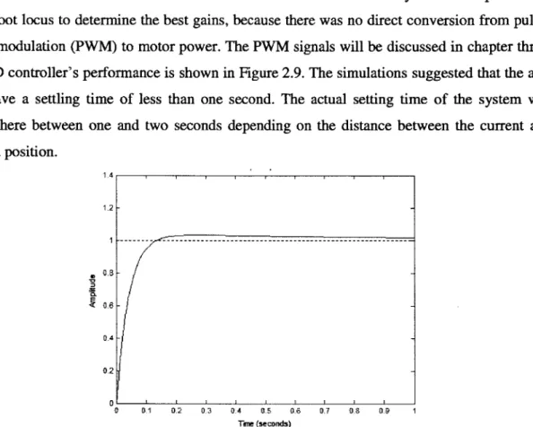
use a root locus to determine the best gains, because there was no direct conversion from

pulse-width-modulation (PWM) to motor power. The PWM signals will be discussed in chapter three.

The PD controller's performance is shown in Figure 2.9. The simulations suggested that the arm

will have a settling time of less than one second. The actual setting time of the system was

somewhere between one and two seconds depending on the distance between the current and

desired position.

Figure 2.9: The settling time of the system with a step input. The simulations suggested

that the arm will move to the desired location within one second.

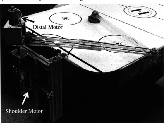
2.5 Complete Mechanical System

The mechanical system served as the structure of the robotic arm. A two-link manipulator

was designed to strike a moving puck with comparable speed and force to that of a person. The

shoulder motor was connected directly to the first link. The distal motor drove the distal arm

through a belt and pulley system. The torque created by the distal motor's mass was eliminated

choice reduced the required motor torque of the shoulder joint motor and lessen the overall cost.

The complete mechanical system is shown in Figure 2.10.

Distal Motor

Figure 2.10: The complete mechanical system; a two-link manipulator that was driven

by two rotational motors. The shoulder joint was directly connected to the first link while

the distal motor drove the distal link through a belt and pulley. This design tried to place

all the mass of the system on the axis of rotation at the shoulder joint.

A bearing support structure was also designed to protect the motors from backlash

and bending moments. Each motor shaft was connected to a drive shaft by a shaft coupler

and then supported at two points by ball bearings. The bearing structure is shown in

Figure 2.11.

Figure 2.11: The bearing support structure for the joint motors. The motors are shown in

teal, the shaft couplers are shown in green, the bearings are shown in red, and the drive

shafts are shown in blue and black. The bearing support structure prevented the motor

shaft from experiencing backlash and bending moments.

Chapter 3

Electrical System Design

The electrical system integrated the controls and sensing aspects of the arm. It took in data

via encoders and a webcam and output the motor commands to an arduino and motor controller.

The electrical system allowed the arm to gather the data from the physical world and used it to

determine the movement of the arm.

3.1 Motor Controllers

The direction of the current and the voltage determines the speed and direction of the motor.

Special circuit boards can be used to manipulate these properties to control the motors. In this

case two circuit boards were used for each motor: a microcontroller and a motor controller. The

motor controller connected a power supply to the motor and provided the circuit necessary to

manipulate the voltage and current. The microcontroller was used to transmit control signals

from a computer to the motor controller.

3.1.1 Motor Controller Selection

The motor controller is a circuit board designed to control the speed and direction of motors.

Important factors to keep in mind are: operational current, maximum current, voltage, and

control signal. It is important to select a motor controller that can operate above the motor

specifications so that the motor controller does not get damaged.

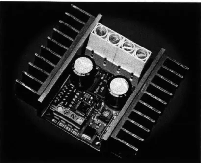
The SyRen 50A Regenerative Motor Controller, shown in Figure 3.1, was chosen to operate

the shoulder motor. This motor controller can handle a continuous 50Amp current, a peak current

of 10OAmps, a 12 Volt input, and a PWM control signal. The shoulder motor operates at 12

Volts with a stall current of 85 Amps. From Figure 2.6, it can be inferred that the maximum

operational current of the shoulder motor will not exceed 50Amps. Therefore, the SyRen 50A

motor control was a suitable motor controller for the shoulder motor.

Figure 3.1: The SyRen 50A Regenerative Motor Controller was selected to control the

shoulder joint.'

The SyRen 10A Regenerative Single Channel Motor Controller, shown in Figure 3.2, was

chosen to drive the distal joint. The distal motor operates at 12 Volts with a stall current of

5

Amps. The motor controller can handle a continuous 10 Amp current, a peak current of 15

Amps, a 12 Volt input, and a PWM control signal. The maximum current draw from the distal

motor will not exceed the peak current. From Figure 2.7, the maximum operational torque is near

the maximum motor power, therefore the motor will not experience a current draw close to the

stall current. As a result, the SyRen 1OA was a suitable choice for the distal motor.

Image courtesy of www.robotmarktplace.com

Figure 3.2: The SyRen lOA Regenerative Single Channel Motor Controller was selected

to control the distal motor.

A microcontroller was used to control the motor controller with PWM signals. The

microcontroller received its information from a computer and output that command as a PWM

signal to the motor controller.

3.1.2 Arduino Microcontroller

A microcontroller is a compact integrated computer. The microcontroller board has

everything it needs in order to run calculation and execute computer codes. It has a processor,

memory, and digital/analog inputs and outputs. The Arduino Uno microcontroller was chosen for

this project, because it was inexpensive and has PWM output pins, a strong support community,

and C language based integrated development environment (IDE).

The microcontroller acted as a relying agent for the motor controller. It received data from a

computer, process it, and sent the motor controller a PWM signal. The Arduino used the code in

Appendix C to actuate the motors.

3.2 Encoders

Quadrature encoders were used to measure the joint angles. The encoders had a spinning

disc with a sensor that recorded "ticks" or markers on the spinning disc. Quadrature encoders

output two signals that can be processed to determine the number of ticks and motor direction.

Figure 3.3 shows an example of the encoder output. The order of the output signals indicates

direction and the frequency of the signals indicates speed [4].

Figure 3.3: A sample output of a quadrature encoder. The order of the two signals

indicates direction and the frequency of the signals indicates speed [4].3

The joint angles were used to calculate the position of the end-effector and determined the

respective joint angular velocities. These measurements were important in determining the

control signals for the PD controller. There were some calibration issues with the encoder that

affect the accuracy of the end-effector. The most notable issues were the rotation of the motor

shafts when the end-effector was physically constrained from moving and the backlash of the

motor shafts. Both of these issues will be discussed later.

3.2.1 Encoder Selection

An E4P OEM Miniature Optical encoder with 100 counts per revolution was chosen for the

shoulder motor. With the gear ratio, this encoder measured 8100 counts per revolution of the

motor shaft. The distal arm had a built-in encoder with 64 counts per revolution. With the

gearhead, this encoder measured 4331 counts per revolution of the motor shaft. The counts per

28

revolution was used to calculate the angle change over time for each joint. The joint angles were

calculated using equation 3.1. This equation states that the current joint angle is equal to the

current joint angle plus the amount of ticks over a time period, ticks, multiplied by a tick to angle

conversion factor. The ticks also took the direction of rotation into consideration.

q

=

q

+ ticks

)

T,

0-0(3.1)

=

q

+ ticks

(43311

3.2.2 Phidgets Highspeed Encoder Board

The PhidgetEncoder HighSpeed 4-Input board was selected to interpret the output signals of

the encoders. The encoder board utilizes a hardware and software interface to allow a computer

to read important information from the encoders via usb. The board takes in the encoder signals

and process it into relative position change, incremental position, and time data. The encoder

information is called upon by the software system to determine the location of the end-effector

and the arm's joint angular velocities.

3.3 Visual System

For the two-link manipulator to be completely autonomous, it needed to be able to detect the

location of the puck in relation to the end-effector. This was accomplished through the use of a

webcam. The webcam was mounted above the manipulator with a field of view of the table

surface. A software system was used to process these images to determine the puck's speed and

position. The puck's speed and position allowed the arm to predict where the puck will be and

how to best reach it. A webcam was chosen because it was affordable and accessible.

3.4 Electrical System Layout

The overall goal of the electrical system was to provide input and output streams for the

software system so that it could control the mechanical arm using real physical parameters.

Figure 3.4 shows a complete diagram of the electrical system.

Webcas

LAPTOP

Ardulno Ulno Mcrocastroler

SyRem 50 A Motr Controer y

Distal Joint Motor/Encoder

Shoulder Joint Motor

Shoulder Joint Encoder

Figure 3.4: A complete electrical system diagram. The blue arrow shows the flow of

data. The computer took in input from the Phidgets encoder board and the webcam and

then output motor commands to the Arduino microcontroller.

The subsystems interacted together to allow the arm to move, track the puck, and determine the

location of the end-effector. The central part of the electrical system was the computer. The

encoders were connected to the Phidgets encoder board which was connected to the laptop. The

Plafget Encoder Beard

motors were connected to the motor controllers, then to the arduino microcontroller and then to

the laptop. The arrangement of the subsystems created a closed-loop feedback of the whole

system.

Chapter 4

Software System Design

The software system acted as the brain of the robotic arm. It gathered data from the

electrical components and decided how to best actuate the mechanical system. The software

system was composed of many separate libraries that functioned together to allow the computer

to process the input data and output the control command in real time. The integration of the

software system allowed the arm to be completely autonomous.

4.1 Boost C++ Libraries and Multi-Threading

The most important subsystem of the software system was the ability to task or

multi-thread. This allowed the computer to process many data input streams, calculations, and output

streams in real time. Without this library, the computer would only be able to execute one

process at a time which would greatly increase the computation time and result in a slower arm

reaction.

Each of the subsystem in the software system existed on a separate thread, and in some

cases, created their own sub-threads. The special thing about the boost library is that it

automatically utilizes the multiple cores in a computer's processor. Once the subsystems use all

the process capability of one core, boost automatically delegate task to the other cores to allow

for continuous data processing and to reduce the delay time between data input and output.

4.2 OpenCV and Visual System

The visual processing subsystem was built with the OpenCV libraries. OpenCV is an open

source, multi-platform software that implements many of the standard image processing

techniques. It is used widely in computer vision applications.

The main OpenCV functions used in this project were: color space transformation, color

detection, image threshold, and contour detection. The color transformation converts an image

from the standard Red-Green-Blue (RGB) color space to the Hue-Saturation-Value (HSV) color

space. The HSV color space was beneficial because it arranges the color in a way that makes it

easier to specify a range of similar colors by only varying one value. The difference between the

RGB and HSV color space is shown in Figure 4.1. The hue determines the color, for example

red, blue, green, yellow. The saturation level defines the intensity of the color. The value

represents the brightness of the color. Both the saturation and value are affected by adding black

or white to the hue.

HSV Color Space

RGB Color Space

Hug

255,5,25

Saturation

Value

Figure 4.1: The HSV color space uses Hue-Saturation-Value to determine a color, while

the RGB color space uses Red-Green-Blue. The HSV color space arrange the colors in a

way that makes it easier to select a gradient of one color.

The color detection algorithm was used to process the image to look for the red puck in the

HSV color space. The image threshold process was used in conjunction with the color detection

algorithm to create a black and white image. The white represented areas on the image where the

color of interest was found. The black represented everything else. By creating this black and

white image, the computer can easily determine where a color is on the image.

The contour detection process took the threshold image and found the boundary lines of the

white spaces. Then a contour area of each contour was calculated and compared so that only the

largest white space was taken into consideration by the software system. This proved to be robust

enough to locate the red puck on the air hockey table through all trials. A sample output of the

vision system is shown in Figure 4.2.

Figure 4.2: The image on the left was captured by a webcam. The software system used

the OpenCV algorithms to locate the red puck and to create a threshold image, shown on

right. It then drew a circle on the captured image to make it easier for the user to see

which object the software system was tracking.

4.3 Phidgets Libraries and Encoders

The Phidgets libraries were used to retrieve the encoder data. The Phidgets encoder board

requires this certain library to communicate with the computer. The Phidgets board took the

encoder signals and created increment position, relative position, and time data. The Phidgets

libraries also created multi-threads in the software system to listen for changes in the encoders

and to notify the software system. This allowed for the real time detection of the end-effector

location.

4.4 Serial Communication and Arduino

The arduino requires a serial communication to exchange data with the computer. The serial

library from www.teuniz.net was selected because it was built for C++ and the call functions

were easy to comprehend. The serial communication link was created on a separate thread that

allowed the arduino and computer to communicate without interruptions. The serial

communication line can only transmit one byte at a time. This meant that only one character

could be sent at a time. For example, if the computer wanted to send "1500" to the arduino, it

would have to break "1500" into four parts: "1", "5", "0", "0". On the arduino end, it would

receive these four bytes, but it would not know that the data should be "1500".

Because of this, a code was implemented on the arduino to sum the data together. In order to

distinguish between the two motors, a motor code was assigned: "a" for the shoulder motor and

"b" for the distal motor. Also, an end signal, "\n" indicating an empty space in characters, was

added to tell the arduino that the computer was done sending data for a specific motor. With this

system, if the computer wanted to send "1500" to the shoulder motor, it would send "a", "1",

"5", "0", "0", "\n". The arduino would read the "a" and assign the resulting value to the shoulder

motor. The complete code and byte calculation is shown in Appendix C.

4.5 Graphic User Interface and Gtkmm

A Graphic User Interface (GUI) is a visual interface that allows a user to interact with the

software system. The same user interface could have been created with only text inputs, but a

GUI was determined to be more effective and easier to use. The GUI allowed for the control of

the arm in manual and autonomous modes and for the input of physical constraints. In the

manual mode, the user could control the motors through the use of the keyboard or text inputs

into the GUI. The autonomous mode disabled the user's control and placed it in the software.

This mode allowed the arm to autonomously play air hockey.

C++ does not come with its own GUI library. GTKmm was selected as an open source GUI

library, because it is cross platform, uses the C++ language, has a GUI builder, and has many

built-in functionality that make the GUI run effectively. GTKmm was used to create the GUI,

along with the interactive buttons, text inputs, and labels. This created an informative, interactive

display for the user in the operation of the arm. The air hockey GUI is shown in Figure 4.3.

Air HOckLy

Conbtr-I.

Figure 4.3: A Graphic User Interface built from the GTKmm libraries. The GUI

consisted of buttons, text inputs, and display labels. The GUI allowed for the control of

the robotic arm.

4.6 Arm Behavior and Controls

The arm's behavior and control thread took in the camera data and the end-effector location

to determine a PD control output. The arm was programmed to strike the puck if it was moving

toward the arm and in an area specified by the software system. If there is no puck or the puck is

moving away from the arm, the arm would go to a home position and wait. The area was

designated to prevent the arm from hitting the edge or getting stuck in its own goal. When the

end-effector hit the edge or was caught in its own goal, the encoders reported change in joint

36

11'5ao

J

0 9 tm Rbo

1

A

ArrnCab~mn- T.--- TtCoto Can-iixto - --

---_______ bcn -4 o- thtwmto fow pptirmtcskvt tw

Amm~ afs -___________)

angles when, in actuality, the end-effector was not moving. The end-effector was physically

constrained by the wall or goal from moving outside the play area, but the motor shaft kept

spinning and caused the shaft couplers or timing belt to slip. This caused the software system to

lose track of the real position of the end-effector and prevented the arm from hitting the puck.

4.7 Software System Layout

The layout of the software system is shown in Figure 4.4. The main thread was the GUI

window. From the main window, other threads were created to handle the various task of the

software system.

Camera

Phidgets

Thread

Thread

Encoder

Listener

Thread

GUI

...

Serial

PD

Update

Thread

Controller

GUI

Thread

Thread

Mcro-controller

Software

Figure 4.4: The layout of the software system. The main thread was the GUI window.

Subsequent threads were created to break up the various task in the software system. The

most important threads are shown in the figure.

The camera thread initialized the webcam to capture a live stream at 30 frames per

second of the air hockey table and puck. It used the OpenCV libraries to process the

images and to determine the puck's location. The position data was passed to a global

variable that was shared among all the threads. The Phidgets thread initialized the

PhidgetEndcoder HighSpeed board and created additional sub-threads to listen for

changes in the encoders and to notify the GUI. The serial thread opened a communication

link via usb between the computer and microcontroller. It was used to pass control

signals from the GUI and PD controller thread to the motor controllers. The PD controller

thread processed the data from the input sensors and determined where the end-effector

should go to hit the puck. The Update GUI thread updated the labels on the GUI to reflect

the real time information.

Chapter

5

Experimental Evaluation

The robotic arm was tested on a Harvard Acclaim 4.6 ft. Air-Powered hockey table. The

table was on the smaller spectrum of air hockey tables, but it was within the design space. The

performance test of the arm began with the mechanical assembly. The two joint motors were

mounted along the rotational axis of the shoulder joint. Then the electrical components were

connected to the mechanical structure to provide the sensory input and output for the software

system. The webcam was mounted above the shoulder joint with an extension on the arm table

mount. An overview of the assembled robotic arm is shown in Figure 5.1.

Figure 5.1: The complete setup of the two-link manipulator system. The two-link

manipulator was mounted on the Harvard Acclaim air hockey table. The electrical

sensors and actuators allowed the arm to autonomously play air hockey. A computer

interpreted the sensory data and used it actuate the mechanical arm.

The shoulder motor was powered by a 12 Volt, 100 Amp PowerMax DC power supply. The

distal motor was powered by a 12 Volt, 3 Amp DC power supply. These power supplies were

chosen to accommodate the stall current of each motor. After many trials, it was observed that

the maximum current on both motors never exceeded 3 Amps. This confirmed that the power

supplies were adequate in providing power to each motors.

Before any testing could be done, the webcam needed to be calibrated to the same

coordinate plane as the end-effector. Four end-effector positions were used to calibrate the

webcam. The four points made a rectangle in the end-effector plane, but a converging

quadrilateral on the camera image. The configuration points are shown in Figure 5.2.

Top View of Air Hockey Table _{Webcam Image of Air Hockey Table}

(XpixeB3,.YpixeB3)

(XreaL3, YreaL3)

(XreaL4, Yreal4)

(3)

0

XpixeWs

(Xpixei1, Ypixel) (XpixeL2. Ypixet2) (Xreali, Yrea ) (Xreal2> Yrea 2)

o1

0

Camera

Figure 5.2: The end-effector plane is shown on the left. Four calibration points were used

to calibrate the camera's perspective to the end-effector coordinate system. The camera's perspective, on right, shows the perpendicular lines of the real system converging to a point near the center.

To compensate for the converging image, a set of linear equations were used to relate the pixel

position, (Xpixei, Ypixet), to real end-effector position, (Xreat,Yrea). Equation 5.1 relates the y

positions.

Yreat =my * Ypixet + by (5.1)

where

__Yreaii-Yreai2

MY

=

_by

_Yreai1

_my

_Ypixei1

The x position required a bit more work because the x-pixel length is dependent on the y values.

Equation 5.2 defines the

xrea

position transformation as a function of the current values

Yreal, Ypixel, and

and calibration points

Xreal

*

Xpixei + bx

(5.2)

where

Xreali - Xrea12

m = C1 - C2 ,

b,

=Xreal1 -mx

c

+

bc

,

Xpixei1

X pixel3

MC

bci

Ypixel.

Ypixel.

Ypixel3

and c

is defined similarly to cl using points 2 and 4.

The purpose of this project was to design and develop a robot that allowed a person to

independently play air hockey. Therefore, the most compelling validation of the robotic arm's

performance is its ability to autonomously hit the puck.

5.1 Performance Validation

The arm was given 73 attempts to autonomously hit a moving puck. To hit a moving puck,

the computer had to calculate a desired striking point. First, it used a center difference method to

find the velocity of the puck. Then, it estimated the puck's position in ten milliseconds using the

current position and velocity vector. Ten milliseconds was experimentally chosen as the time

step, because it gave the arm enough time to reach the puck from anywhere on the table. Out of

the 73 attempts, the arm was able to strike 50 pucks resulting in a 68.5 percent hit rate. This was

an excellent result for the first prototype. Due to the complexity of the system and the simplicity

of the controls, the hit rate was expected to be lower than 10 percent.

The behavior of the arm was observed to follow the programmed behavior and controls. The

arm did not attempt to strike at pucks that were moving away from it or too close to the walls. It

returned to its home position after every attempt and did not move when there was no puck

present.

Although the results were promising, there were many issues in the operation and

controls of the robotic arm. The largest issue was the misalignment of the end-effector position

and the calibrated camera position. Sometimes, the motor overshot the puck's position and hit

one of the side walls. In this case, the motors kept rotating but the end-effector did not move. As

a result, the computer lost track of the real end-effector position and could not hit the puck

accurately.

Another issue was the backlash in the joint motors. The distal arm had a five to ten

degree of rotation before the encoder registered any movement. The shoulder motor had even

greater backlash. The backlash also resulted in miscalculations of the end-effector position.

Chapter 6

Summary and Conclusion

Air hockey is a sport that is usually played between two or more individuals. There is an

inherent issue with the dependency of another person. Sometime, it is more favorable to play air

hockey by oneself. An autonomous robotic arm was designed and developed to allow a person to

independently play air hockey. The robotic arm consisted of three main systems: mechanical,

electrical, and software. The mechanical system was designed as a two-link manipulator with

Proportional-Derivate

position

control.

The electrical

system

contained

encoders,

a

microcontroller, motor controllers and a webcam. The encoders were used to determine the joint

angles. The microcontroller and motor controllers were used to actuate the joint motors. The

webcam was used to track the position of the puck. The software system used the sensory data

to control and actuate the mechanical system.

The robotic arm's performance was well above the expected value. The arm had a hit rate of

68.5

percent and behaved as expected. This indicated that the arm was not hitting the puck by

chance. The result suggests that the arm will be able to autonomously play air hockey, but it

could be improved by making a few adjusts as outlined in the future work.

6.1 Future Work

Many improvements can be made to increase the performance and robustness of the

robotic arm. The major issue that needs to be addressed is the calibration between the real and

calculated end-effector position. A more sensitive encoder, more ticks per revolution, might be

able to resolve the miscalibration issues. It is also possible that the bearing support structure and

shaft couplers are not rigid enough to transfer the rotation of the drive shaft to the motor shaft

and encoder.

Instead of a hardware fix, a software solution might prove to be the better option. The

webcam can be programmed to track the puck and end-effector in the pixel coordinate system. A

control loop can be found to move the end-effector to any desired pixel coordinate. In this

solution, the location of the puck and end-effector will always be known and in the same

coordinate system. This should prevent the miscalibration issues of a calculated end-effector

position that only depended on the encoders. The encoder will still be useful as a velocity sensor

and secondary estimate of the end-effector position.

Other secondary improvements can be made to the camera, controller design, and

behavior and strategy. Through experimental observation, the current camera at 30 frames per

second was not able to track fast moving pucks. A faster camera capable of capturing more

frames per second can give the software system a better estimate of the real position and velocity

of the puck. A more complex controller design that takes into account the dynamics and

kinematics can also improve the arm's performance. And lastly, the arm's behavior and strategy

can be improved to make the arm play at a more realistic and competitive level.

Bibliography

[1] Dazadi, "Air Hockey History," 18 Feb 2009, www.dazadi.com (24 April 2013).

[2] George Konidaris

et

al., Math, Numerics, & Programming (for Mechanical Engineers), 2011.

[3] S. Colton. Notes on DC Motors. 2011.

[4] Pololu Robotics & Electronics, "67:1 Metal Gearmotor 37Dx54L mm with 64 CPR

Encoder," 2013, www.pololu.com (26 April 2013).

%%this script is used to process velocity and acceleration of puck/striker%%

%clean workspace

close all clear all

clc

%load data (the coords are in mm) %column 1 = marker number

%column 2 = x coord %column 3 = y coord

%column 4 = z coord %column 5 = blank

load('puck3.mat');

figVar = figure; %create figure MarkerPosVar = MarkerPosVar/1000; %V = 1/(2h) *

(

)

Velocity = zeros(iCounter-1,2); %x and y velocity

1. 2. 3. 4. 5. 6. 7. 8. 9. 10. ll. 12. 13. 14. 15. 16. 17. 218. 19. 20. 21. 22. 23. 24. 25. 26. 27. 28. 29. 30. 131. i 32. 33. 34. 35. 36. 37. 38. 39. 40. 41. 1,3) end end

Velocity(i,2) = 1/(2*timeLap(i)) *

(

%y velocity

-

MarkerPosVar(i--

MarkerPosVar(i-i+1,2) -

MarkerPosVar(i-i+1,3) -

MarkerPosVar(i-VelMag sqrt(Velocity(:,1).A2 + Velocity(:,2) A2);

tempA = find( VelMag > 20); VelMag(tempA) = [] plot([1:size(VelMag,1)],VelMag); xlabel('Time (s)') ylabel('Speed (m/s)')

Appendix A

Matlab Code

1:(iCounter-1)

if

i

Velocity(1,2) =

l/timeLap(1)

MarkerPosVar(2,3)

MarkerPosVar(1,3)

elseif i == (iCounter - 1) %do backward difference

Velocity(i,1) = 1/timeLap(i) *

(

)

Velocity(i,2) = 1/timeLap(i) * ( MarkerPosVar(i,3)

1,3) ); %y velocity

else %do centered difference

Velocity(i,1) = 1/(2*timeLap(i)) *

(

);

42. %43. 44. 45. 46. 47. 48. 949. 50. S51. 52

~53.

load(

81.

title('Puck Velocity Histogram');

95. puckAccelFig = figure;

96. {puckN2,puckXOut2] = hist(allPuckAcc,20); 97. bar(puckXOut2,puckN2/size(allPuckAcc,1));

98. xlabel('Acceleration(m/s^2)');

99. ylabel('Frequency')

100. title('Puck Acceleration Histogram');

elMag]; .k3AccelMag];

48

fig2 = figure; %acceleration figure accel = zeros(iCounter-3,2);

for i = 2:(iCounter-2)

accel(i-1,1) = (1/timeLap(i)42) *

(

);

accel(i-1,2) = (1/timeLap(i)A2) * ( MarkerPosVar(i-1,3)

-2*MarkerPosVar(i,3) + MarkerPosVar(i+1,3) ); %y accel

end

Accel.Mag = sqrt( accel(:,1).^2 + accel(:,2)^2 )A tempB = find( AccelMag > 200);

AccelMag(tempB)= plot([1:size(AccelMag,i)],AccelMag); xlabel('Time (s)') ylabel('Acceleration (m/sA2)') title('Striker Accel') fig3 = figure; mass-puck = 12.4/1000;

force = massipuck * accelMag;

plot(time(2:iCounter-2),force); xlabel('Time (s)') ylabel('Force (N)') title('Striker Force') %}

'

'