Design of a 250 GHz gyrotron amplifier

Design of a 250 GHz Gyrotron Amplifier

by

Emilio A. Nanni

B.S. Electrical Engineering, University of Missouri

-

Rolla (2007)

B.S. Physics, University of Missouri

-

Rolla (2007)

Submitted to the

Department of Electrical Engineering and Computer Science

in partial fulfillment of the requirements for the degree of

Master of Science

at the

MASSACHUSETTS INSTITUTE OF TECHNOLOGY

September 2010

ARCHIVES

O

E'T

/1

OCT

a 5

2

i

@

2010 Massachusetts Institute of Technology. All rights reserved.

/

Authoi ...

.

Department of Electrical Engineering and Computer Science

August 17, 2010

Certified by ...

...

Richard J. Temkin

Senior Research Scientist, Department of Physics

Thesis Supervisor

A ccepted by ...

'Professor Terry P. Orlando

Chairman, Committee on Graduate Students

Department of Electrical Engineering and Computer Science

Design of a 250 GHz Gyrotron Amplifier

by

Emilio A. Nanni

Submitted to the Department of Electrical Engineering and Computer Science on August 17, 2010, in partial fulfillment of the

requirements for the degree of Master of Science

Abstract

A design is presented of a 250 GHz, 1 kW gyrotron traveling wave tube (gyro-TWT)

amplifier with gain exceeding 50 dB. Calculations show that the amplifier will operate at 32 kV, 1 A with a saturated gain of 60 dB, an output power of 1 kW and a gain bandwidth of 3 GHz. The amplifier uses a novel photonic band gap (PBG) interaction circuit for stable single mode operation in an overmoded circuit. The design mode is a TE0 3-like mode confined by the PBG lattice with no nearby competing modes. The

design of the input coupler, interaction circuit, output coupler and electron gun have also been completed. The amplifier design accounts for requirements imposed by the device's intended application of pulsed nuclear magnetic resonance spectroscopy with pulses as short as several hundred picoseconds. This design will be implemented at a later date for the construction of the highest frequency, kW power level amplifier based on vacuum electronics. To gain understanding of short pulse amplification in vacuum electron devices, an experimental study of sub-nanosecond pulse amplification in a gyro-TWT has been carried out on an existing experimental setup at 140 GHz. The gyro-TWT operates with 30 dB of small signal gain in the HE06 mode of a confocal

waveguide. Picosecond pulses show broadening and transit time delay due to two distinct effects: the frequency dependence of the group velocity near cutoff and gain narrowing by the finite gain bandwidth of 1.2 GHz. Experimental results taken over a wide range of parameters, with pulses as short as 400 ps, show good agreement with a theoretical model in the small signal gain regime.

Thesis Supervisor: Richard J. Temkin

Acknowledgments

I would like to thank my advisor, Dr. Richard Temkin, for his guidance and

men-torship. He never fails to provide good suggestions and is an invaluable source of knowledge. I would also like to thank Dr. Michael Shapiro for many useful conver-sations and for patiently answering all of my questions, and Dr. Jagadishwar Sirigiri for all his help in the lab and for keeping me on track. I have benefited from working with all of our group members: Dr. Alan Cook, Dr. Hae Jin Kim, Dr. Colin Joye, Elizabeth Kowalski, Dr. Roark Marsh, Ivan Mastovsky, Brian Munroe, David Tax and Antonio Torrezan de Sousa. You have made this process so enjoyable. I want to thank my instructor for all things DNP, Alexander Barnes. I could never forget my mentors Dr. Reza Zoughi and Dr. Ronald Bieniek, both from the University of Missouri-Rolla, who encouraged me to be a better student, scientist and engineer. On a personal note, I must also thank my parents Antonio and Valeria Nanni who in-spired me and provided me with every opportunity. Finally, my fiancee Sarah Wilson, your love is all the support I will ever need.

Contents

1 Introduction

1.1 M otivation . . . . 1.2 Gyrotron Oscillators and Amplifiers . . . . .

1.3 Background of Gyro-TWTs . . . .

1.4 Current Effort . . . .

2 Theory of Gyro-devices

2.1 Axial and Azimuthal Bunching of Electrons . . . . 2.2 Fundamentals of Gyrotron Oscillators . . . .

2.3 Background . . . . . . . ..

2.4 Nonlinear Theory of Gyrotron Oscillators . . . . 2.4.1 Derivation . . . . 2.4.2 Analysis... . . . . . . .. 2.5 Quantum Mechanical Approach for Gyrotron Oscillators

2.6 Theory of Gyrotron Traveling Wave Tubes . . . . 2.7 Short Pulse Propagation and Amplification . . . . 2.8 Conclusion . . . . 3 250 3.1 3.2 GHz Gyro-TWT Design Introduction . . . . . . . .. Attenuation in Waveguides . . . . 17 . . . . 17 . . . . 18 . . . . 20 . . . . 2 2 25 . . . . 25 . . . . 28 . . . . 30 . . . . 32 . . . . 32 . . . . 37 . . . . 40 . . . . 43 . . . . 45 . . . . 52 53 53 55

3.3 Photonic Band Gaps . . . . 57

3.4 PBG Interaction Circuit . . . . 62

3.5 Linear Growth Rate . . . . 68

3.6 Input Coupler . . . . 75

3.7 Output Coupler . . . . 77

3.8 Electron Gun . . . . 79

3.9 Conclusion . . . . 88

4 Short Pulse Amplification 89 4.1 Introduction . . . . 89

4.2 Experimental Setup . . . . 92

4.3 Short Pulse Amplification... . . . . . . . 93

4.3.1 Pulse Broadening Curves . . . . 99

List of Figures

2-1 The solution to 2.5 for Ge/Yowp = 10 and -yo = 1.02. . . . ... 27

2-2 Cross section of the interaction region along the axis of the DC mag-netic field with (a) a view of the electron beam passing through the physical structure, (b) the amplitude (c) and phase of the RF electric field and (d) the DC magnetic field [26]. . . . . 29 2-3 Dispersion diagram for cyclotron resonance and cylindrical waveguide

m odes. . . . . 30

2-4 Power output for vacuum electron and solid state devices [42]. . . . . 31 2-5 Cross section of the interaction region with black dots representing

electrons on their gyration orbit [27]. The waveguide radius is ro, the Larmor radius is rL, the guiding center radius is Re and EO denotes the 9 component of the electric field... . . . . . . ... 33 2-6 Contour plot for efficiency of the 1" harmonic interaction between a

cavity with normalized field strength, F, and interaction length, p. . . 38 2-7 Contour plot for efficiency of the 2"d harmonic interaction between a

cavity with normalized field strength, F, and length, p. . . . . 39

2-8 The fraction of electron energy that is extracted from the beam,

aver-aged over 32 initial phases, as it passes through the cavity. . . . . 40

2-9 Stimulated emission of an electron in a magnetic field with relativistic

3-1 Dispersion relation for a circular waveguide with a 2 mm radius. . . . 54

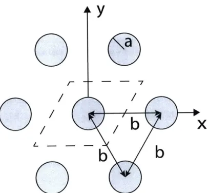
3-2 Triangular lattice of metallic rods. The fundamental unit cell is marked

with a dashed line. . . . . 58 3-3 Reciprocal triangular lattice where b' = -,. The gray area is the

73b

irreducible Brillouin zone. . . . . 58

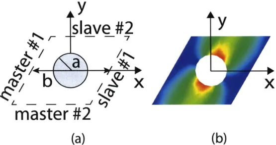
3-4 (a)Master/slave boundaries for the unit cell and (b) the equivalent

HFSS model with the complex magnitude of the electric field of the

lowest order propagating mode for a/b = 0.2,

#1

#1

3-5 Normalized eigenmode frequencies as a function of ki for a/b = 0.2. 61 3-6 Normalized eigenmode frequencies as a function of ki for a/b = 0.43. 61 3-7 The global band gap plot for a triangular lattice, where a is the spacing

and b is the diameter of the rod. . . . . . . . . . 62 3-8 The global band gap plot with the operational spacing of a/b = 0.43

is marked with a dashed red line. The TE03 mode for a finite lattice

with three rods removed is marked with a red point. . . . . 64

3-9 The complex magnitude of the electric field for the TE_{0 3} mode confined in a circular waveguide. . . . . 66 3-10 The complex magnitude of the electric field for the TE_{0 3}-like mode

confined in a PBG composed of a triangular lattice of metal rods. . . 66 3-11 Attenuation as a function of frequency for the TE0 3-like mode. . . . . 67 3-12 Normalized coupling coefficient comparison for a circular waveguide

and the PBG waveguide. The electron beam radius for the gyro-TWT w ill be 1.1 m m . . . . 67 3-13 Gain in dB/cm from linear theory. . . . . 70

3-14 Gain in the device calculated from the linear growth rate and loss per unit length of the circuit. Reflections are suppressed enough to prevent oscillations. . . . . 70 3-15 Gain in dB/cm at 250 GHz as a function of perpendicular velocity

3-16 Gain in the device calculated from the linear growth rate for a 22 cm

circuit compared to results from MAGY for a 26 cm circuit with 5%

perpendicular velocity spread. . . . . 73

3-17 Dimensions of circuit simulated in MAGY. . . . . 73

3-18 Output power as a function of frequency simulated with MAGY using a 32 kV, 1 A electron beam with 5% v1 spread. . . . . 74

3-19 Output power as a function of the input power for 250 GHz. . . . . . 74

3-20 Band gaps in at triangular lattice. . . . . 76

3-21 S-parameters for the wraparound input coupler. . . . . 76

3-22 Uptaper dimensions simulated and optimized in CASCADE. . . . . . 78

3-23 S1 of the uptaper for the TE0 3 mode. . . . . 78

3-24 S21 of the uptaper for the TE0 3 mode.. . . . . 78

3-25 Gun parameters calculated using equations derived by Baird and Law-son for a 32 kV 2 A beam and 50 degree cathode tilt. The (a) compres-sion, (b) magnetic field at the emitter, (c) emitter width, (d) maximum electric field and cathode to mod-anode potential, (e) Langmuir space charge, and (f) cathode to mod-anode spacing, d, and guiding center spread are plotted versus the mean emitter radius. Black dots mark the selected design values. . . . . 81

3-26 Schematic of the electron gun design with all units in mm unless oth-erwise m arked. . . . . 81

3-27 The magnetic field as used to model the electron gun performance. The guiding center radius is also plotted along the axis of the magnet. 83 3-28 The main magnetic field with the gun coil magnet at 0% and ±25% of the rated current. . . . . 83

3-29 Electric field distribution for the cathode at -32 kV, mod-anode at -18kV and anode at ground. . . . . 84

3-30 Electric potential lines and particle trajectories for the cathode at -32 kV, mod-anode at -18kV and anode at ground. Gun coil at 25% of rated current. . . . . 84

3-31 Cross sectional CAD drawing of 9.6 Tmagnet. . . . . 86 3-32 Operational parameters for the electron gun at 32 kV. Gun coil at 25%

of rated current. . . . . 86 3-33 Operational parameters for the electron gun at 40 kV. Gun coil at 25%

of rated current. . . . . 87

3-34 Operational parameters for the electron gun at 50 kV. Gun coil at 25% of rated current. . . . . 87

4-1 Dispersion diagram of HE0 6 gyro-TWT in a confocal waveguide (left)

and cross sectional view (right). The annular electron beam has a 4.2 mm diameter... . . . . . . . . . . . . . 90

4-2 Measured (dots) and calculated (solid line) gain-bandwidth curve for a beam voltage of 28 kV. . . . . 91

4-3 Measured (dots) and calculated (solid line) gain-bandwidth curve for a beam voltage of 35.4 kV. . . . . 91

4-4 Measured input and output power at 137.8 GHz for the 35.4 kV oper-ating point. The gain is 23.5±0.34 dB . . . . 92

4-5 Schematic diagram of the picosecond pulse amplification in a quasiop-tical gyro-TW T . . . . 93

4-6 Attenuation as a function of frequency in a 10 cm section of WR4 w aveguide. . . . . 95

4-7 Measured (dots) and calculated (solid line) transit time delay of 500 ps pulses in (a) 10 cm long WR4 waveguide with a cutoff frequency of 139.25 GHz and (b) the 28.4 cm gyro-TWT confocal waveguide structure with a cutoff frequency of 135.0 ± 0.3 GHz. . . . . 96

4-8 Output pulse width as a function of input frequency for 10 cm WR4 waveguide and a constant input pulse width of 500+25 ps. . . . . 96

4-9 Output pulse width as a function of input frequency for a beam voltage of 28kV and a fixed input pulse width of 425±25 ps . . . . 98

4-10 Pulse shapes for an input pulse of 580 ps at the 35.4 kV operating point. The output pulse at (a) 137.3 GHz has a measured width of

1045 ps and (b) at 138.13 GHz has a measured width of 660 ps. . . . 98

4-11 Measured (dots) and calculated (solid lines) output pulse width after amplification as a function of input pulse width for 28 kV and (a) 136.94 GHz, (b)137.4 GHz, (c) 137.92 GHz and (d)138.2 GHz. . . . . 100

4-12 Measured (dots) and calculated (solid lines) output pulse width af-ter amplification as a function of input pulse width for 35.4 kV and (a)137.3 GHz, (b)138.13 GHz and (c)138.8 GHz. . . . . 101

List of Tables

1.1 Recent Gyro-TWT Experiments ... ... 21

2.1 Illustrative THz Gyrotron Oscillator Experiments . . . . 31

3.1 Simulation Parameters to Investigate Brillouin Zone . . . . 60

3.2 Design Operating Parameters from Linear Theory . . . . 69

3.3 Design Operating Parameters from MAGY.. . . . . . . . . 72

Chapter

Introduction

1.1

Motivation

Novel high power sources in the millimeter and sub-millimeter wave are of great in-terest due to their potential applications in spectroscopy, communications and radar. This thesis presents the design of a 250 GHz, 1 kW gyrotron traveling wave tube am-plifier for nanosecond pulses with gain exceeding 50 dB. The amam-plifier will eventually be used in pulsed dynamic nuclear polarization (DNP) nuclear magnetic resonance (NMR) and electron paramagnetic resonance (EPR) experiments. Controlled mi-crowave irradiation of an NMR sample can be used to transfer the high electron polarization to the nucleus under study resulting in a dramatic increase in the NMR signal by factors exceeding 100 [3]. Currently, there are no commercially available devices that can generate peak powers in the kW region with high gain at 250 GHz.

A gyrotron amplifier was chosen because it offers high gain, broad bandwidth at

these frequencies and allows the use of an overmoded interaction structure resulting in easier fabrication and reduced thermal effects.

Pulsed DNP NMR requires the amplification of pulse trains with ns times scale resolution. In principle an amplifier with over 1 GHz of instantaneous bandwidth should be able to meet this requirement. However, waveguide dispersion and gain dispersion remain a concern for successful operation. In light of these concerns a study of pulse amplification in a 140 GHz gyrotron traveling wave tube (gyro-TWT) was

performed. The 140 GHz gyro-TWT used in the experiment was developed at MIT for use in pulsed DNP. This study was the first investigation of sub-ns pulse amplification in a gyro-TWT, and yielded the first dispersion free amplification of sub-ns Gaussian pulses. The effects of waveguide dispersion and gain dispersion were thoroughly investigated in the linear gain regime of the amplifier. A theory was developed to describe the effects of waveguide and gain dispersion on pulse amplification in gyro-TWTs, in excellent agreement with experimental results.

1.2

Gyrotron Oscillators and Amplifiers

The generation of millimeter and sub-millimeter wavelength radiation at high power has proved to be a significant challenge. Solid state devices have never been considered as a possibility for high power generation at such high frequencies (hundreds of GHz) due to scalability and efficiency issues. Classical microwave tubes, e.g. klystrons and traveling wave tubes, can produce high power (kW) electromagnetic radiation up to

100 GHz, but these slow wave devices require physical structures in the interaction

cavity that are smaller than the wavelength of operation. This small element size produces difficulties with thermal damage and manufacturing of the interaction cav-ity. Gyrotrons are a form of electron cyclotron maser capable of producing kilowatts to megawatts of output power in the microwave, millimeter wave and terahertz bands

[18, 12, 22, 36]. These devices operate by the resonant interaction between the

eigen-modes of an interaction cavity, typically cylindrical, and a mildly relativistic electron beam that is gyrating in a constant axial magnetic field. The most basic configuration of a gyrotron consists of a magnetron injection gun (MIG) that launches an annular electron beam into the hollow bore of a solenoidal, often superconducting, magnet. The orientation of the DC electric field that extracts the electron beam from the cath-ode produces a beam that has both a perpendicular and parallel velocity component to the axial field produced by the solenoidal magnet. As the electron beam travels into the central bore, it undergoes adiabatic compression that increases its orbital momentum. The beam enters a metallic cavity that has an eigen-mode resonance

that is close to a harmonic of the frequency at which the electron gyrates around the magnetic field line. The electron beam surrenders some of its kinetic energy to the electromagnetic mode through stimulated emission. The electrons exit the cavity and are deposited on a metallic collector. In its simplest configuration, the collector can also hold an axial dielectric window that couples the electromagnetic radiation out of the device. However, it is often convenient to convert the wave into a Gaussian beam that can be efficiently extracted in a transverse direction using mirrors.

In recent years, gyrotron traveling wave tube (TWT) amplifiers have demonstrated high output power levels with significant gain bandwidths [13, 11, 7]. A gyrotron-TWT amplifier works on the same fundamental principles as a gyrotron oscillator for the extraction of energy from an electron beam. However, the amplifier is operated under conditions that suppress self-start oscillations, including backward wave oscilla-tions (BWOs) that could disrupt the operation of the device. Amplification is achieved in a gyro-TWT by a convective instability supported by a mildly relativistic, annular, gyrating electron beam and a transverse electric mode in a waveguide immersed in a strong static axial magnetic field

(BO).

w - sG/7 - kzvz 0 (1.1)

and the waveguide mode dispersion relation is expressed as

w

_-

_k

_c

_{- k}

_c

_(1.2)

z I

where w is the frequency of the wave, Q = eBo/me is the non-relativistic cyclotron

frequency of the gyrating electrons, e and me are, respectively, the charge and the rest mass of the electron, -y is the relativistic mass factor, s=1 is the cyclotron har-monic number, k, and ki are the longitudinal and transverse propagation constants, respectively, of the waveguide mode, vz is the axial velocity of the electrons, and c is

the velocity of light. This requires the design of an interaction circuit that supports the propagation of a mode at the correct frequency while appearing lossy to frequen-cies and modes outside the region of interest. This is usually performed by inserting lossy ceramics, severs and selecting geometries with favorable dispersion relations

[29]. Further complications arise when considering the design of an amplifier at 250

GHz because the operational mode of the amplifier cannot be a fundamental mode due to compression restrictions of the electron beam. In a gyro-TWT, the signal of interest must be efficiently coupled into the cavity at the beginning of the interaction region. The wave propagates along the amplifier circuit while extracting energy from the electron beam until it is removed from the device with an output coupler in a similar fashion to the oscillator.

1.3

Background of Gyro-TWTs

Gyro-TWT amplifiers were first studied in the early 1970s, mainly at the Naval Re-search Laboratory (NRL). These devices were in the X and Ku bands and operated in the fundamental waveguide mode [4, 39]. These early studies showed how the promise of high gain and high output power in gyro-TWTs was limited by the strong forward and backward wave gyrotron oscillations near the waveguide cut-off and interaction at higher harmonics.

More recently, a scheme of distributed loading was proposed by the research group at the National Tsing Hua University (NTSU) in Taiwan to suppress the gyrotron backward wave oscillations (gyro-BWO) and forward wave gyrotron oscillations near the waveguide cut-off. A proof-of-principle device demonstrated over 70 dB of gain at

35 GHz [13]. This device operated in the fundamental TE11 waveguide mode.

Subse-quently, a TEOi high average power device based on this concept was demonstrated at NRL [35] and a TEOi device was demonstrated at 94 GHz by Communication and Power Industries (CPI) [8]. A comparison of recent gyro-TWT experiments is shown in Table 1.1.

Table 1.1: Recent Gyro-TWT Experiments

Freq (GHz) Gain (dB) Pout (kW) Voltage (kV) Current (A)

NTHU[13] 35 70 93 100 3.5

CPI[8] 95 43 1.5 30 1.8

MIT (2003)[42] 140 29 30 65 7

MIT (2008)[29] 140 34 0.8 37 2.7

However, operation at fundamental modes is not feasible at high frequencies such as 250 GHz where the radius of the interaction structure would be of the order of a fraction of a millimeter. This results in high ohmic losses and presents significant challenge in transporting an electron beam over long distances (~20 cm) without causing beam interception on the waveguide walls. In prior research at MIT, gyro-TWTs with high power (30 kW) and low power (0.8 kW) have been successfully demonstrated at 140 GHz [44, 29]. These experiments used a novel quasioptical, overmoded interaction structure which allows for single mode operation in a higher order mode. The interaction circuit consists of a confocal waveguide with severs for additional suppression of oscillations. Such a mode-selective open waveguide imparts high diffractive losses to the lower order modes which tend to interact with the beam more strongly. This selective loading of the lower order modes allows for stable operation in a higher order mode. Though mode selective, the confocal waveguide has an azimuthally asymmetric field profile which reduces its interaction efficiency with the annular beam produced by the MIG that is typically used in gyrotrons.

One important application of millimeter waves is in spectroscopy, where coherent pulses on a sub-nanosecond or picosecond time scale are needed for optical pumping of molecular states. The pulses must be shorter than the relaxation time, typically requiring sub-nanosecond (or picosecond scale) pulse lengths [6]. Sub-nanosecond microwave pulses have been demonstrated in a vacuum electron device by superradi-ance [21], but such pulses cannot be used for spectroscopy. Sub-nanosecond pulses must contain a spectral bandwidth exceeding the transform limit of 1 GHz. In the conventional microwave bands at frequencies of one to several GHz, the required gain bandwidth to amplify such picosecond pulses is generally not available, since the GHz

bandwidth is a large fraction of the carrier frequency. In recent years, high power, wideband amplifiers in the millimeter wave band have been developed that are suit-able for amplifying picosecond pulses. For example, a form of klystron called an extended interaction klystron has been developed at 95 GHz with a gain bandwidth of about 1 GHz. This amplifier has been used to successfully amplify 1 kW output pulses as short as 800 picoseconds [9]. A gyro-TWT at 95 GHz has been demon-strated with a gain bandwidth of 6.5 GHz at an output power level of 2 kW [7]. This gyro-TWT could in principle be used to amplify a 150 ps pulse. To our knowledge, amplification of picosecond pulses has not been tested with these or other powerful wideband gyro-amplifiers. Because of the possibility of distortion in amplification of picosecond pulses, detailed studies are needed of the amplification process in such devices.

1.4

Current Effort

A novel interaction structure that is highly mode selective and has strong coupling

with the electron beam resulting in higher interaction efficiency will be presented. The circuit is based on a photonic band gap (PBG) structure made of a two dimen-sional triangular lattice of metal rods. The dimensions of the lattice are tuned so that it acts as a perfect reflector in a narrow band of frequencies around the oper-ating mode. A defect is created in the lattice by removing some rods, allowing a higher order mode to be confined with high a quality factor (Q). Other modes that can exist in the defect either at higher or lower frequencies suffer significant losses because of the partially transparent lattice. This amplifier will ultimately be applied to coherent molecular spectroscopy. Therefore, the bandwidth of the amplifier has been an important consideration to insure the ability of the gyro-TWT to faithfully amplify very short pulses without distortion, since it is important to the application. The input coupler, output coupler and electron gun designs for this experiment will be presented.

kW, 140 GHz gyro-TWT with a gain bandwidth exceeding 1 GHz. The gyro-TWT operates with 30 dB of small signal gain near 140 GHz in the HE06 mode of a confocal

waveguide. Picosecond pulses show broadening and transit time delay due to two distinct effects: the frequency dependence of the group velocity near cutoff and gain narrowing by the finite gain bandwidth of 1.2 GHz. A comparison between theory and experiment in the dispersion of picosecond pulses in a vacuum electron device amplifier was performed by driving the amplifier with pulses as short as 400 ps, which contain frequencies over a 2.5 GHz bandwidth, about twice the amplifier's inherent gain bandwidth. Experimental results show good agreement with a theoretical model in the small signal gain regime. These results show that in order to limit the pulse broadening effect in gyro-amplifiers, it is crucial to both choose an operating frequency at least several percent above the cutoff of the waveguide circuit and operate at the center of the gain spectrum with sufficient gain bandwidth.

Chapter2

Theory of Gyro-devices

2.1

Axial and Azimuthal Bunching of Electrons

An electron beam propagating along a magnetic field line is subject to a variety of instabilities. Of particular importance are the axial and azimuthal bunching mech-anisms of the electromagnetic electron cyclotron instability. The electron cyclotron maser instability is driven by the azimuthal bunching mechanism and requires a rel-ativistic treatment. The Weibel-type instability is driven by axial bunching and does not require relativistic treatment. Both mechanisms exist and compete against each other when an external magnetic field is present [15].

Assume an infinite homogeneous magnetic field Bos with the electron distribution given by

fo = 6(p_ - pio)6(p2)/27rp1 (2.1)

where pi is the transverse momentum, p, is the axial momentum and pLo is a con-stant. This distribution represents streaming electrons in the moving frame. This monoenergetic beam would be the ideal case for an experiment designed to extract energy from the electrons, and it approximates the electron beam produced by high quality electron guns.

require the linearized relativistic Vlasov equation,

a

a

e

a

1

a

fi+v---f1--vxBo-

fi=e

fo

at

8x

c

89p

c

ap

and the combined Maxwell's equations,

1

82

47r

a

V

V

Ei =

E -

J

(2.3)

c2 at2 c2 2t

to fully describe the physics of the interaction. A subscript 0 or 1 represent the initial or perturbed quantity, respectively. The electron distribution is f, E is the electric field, B is the magnetic field, and the current J is defined as

J = -e Ifivd3P.

Simplifying the above equations and performing perturbative analysis for a wave that propagates as exp(-iwt + ikzz), we obtain the relativistic dispersion relation [15]:

2C2 = -rw pidpj

dpz

kzpz

afo

kz

afo

(-xKW

-)/

pi''

+

-k"1--- (yo-

kzpz/m

-

where w2 = 47rne2/m,

Qe =

/m

expression is for any generic distribution of the electrons. However, we can

sim-plify further by considering the monoenergetic case from Equation (2.1) that is most

relevant to practical devices. This reduces the dispersion relation to

2 2 _ "2 W #i2 -kc2

w2

-

k c

(2.5)

Z

yo

-

,

2(uo

where -yo = (1 + piO/m 2_c2

)1_/2 _and

_#10o

inter-pretation from Equation (2.5) one should make note that the last term on the RHS is where the axial and azimuthal bunching mechanism reside. The azimuthal and axial bunching are represented by the w2 _{and c}2_{k2 terms respectively. Furthermore, the}

denominator (w - Ge/yo) imposes a requirement that the frequency of oscillation for

the wave must meet the condition w ~ Ge/Yo in order to produce a large instability.

This can be understood as a requirement for synchronous behavior between the

elec-trons and the electromagnetic wave. Additionally, if the phase velocity of the wave is

equal to the speed of light there is no instability present, defining an inflection point

between an instability dominated by axial and azimuthal bunching. If

W2/k > C2,

(2.6)

the phase velocity of the wave is greater than the speed of light and azimuthal

bunch-ing dominates. If

w2

_{/k <c}

,

(2.7)

the phase velocity of the wave is less than the speed of light and axial bunching

and yo

=

1.02. We note that the instability is only present when the frequency of

the fast and slow wave meet the condition w/w,

=

10 as required for synchronous

behavior. The instability for the fast and slow wave are only present when Equations

(2.6) and (2.7) are satisfied.

C.

5 10 15

k c/o

z p

20 25

Figure 2-1: The solution to 2.5 for Qe/yowp = 10 and yo = 1.02.

Fast Waveo_r Fast Wave 1 On. Slow Wave o_r

- -Slow Wave 1 00io.

Gyrotrons and gyro-TWTs are both fast wave devices that rely electron cyclotron maser instability, driven by the azimuthal bunching mechanism. Due to this bunching mechanism a relativistic treatment is required to explain these devices properly.

2.2

Fundamentals of Gyrotron Oscillators

As mentioned in the previous section, electron cyclotron resonance masers (gyrotrons) are fast wave devices, i.e. the phase velocity of the wave is greater than the speed of light. They are capable of producing high average power in the microwave, millimeter wave and sub-millimeter wave range. The most basic configuration of a gyrotron can be seen in Figure 2-2. The magnetron injection gun that launches an annular electron beam would be located to the left of Figure 2-2(a). The axial magnetic field is produced by a solenoidal magnet than can either be a pulsed magnet or a DC superconducting magnet. As the electron beam travels through the central bore, it enters a metallic cavity that has an eigen-mode resonance that is close in frequency to a harmonic of the frequency at which the electron gyrates around the magnetic field line. The electron beam surrenders some of its kinetic energy to the electromagnetic mode through stimulated emission. In order for the electron to interact with the electromagnetic mode in the cavity, the relativistic electron frequency must be close to the frequency of oscillation for the mode [14]. The relativistic cyclotron frequency is

Qrei = eB0 (2.8)

'Yme

where B0 is the DC axial magnetic field, 'y is the relativistic mass factor, me is the

electron mass, e is the charge of the electron. In a cylindrical cavity the dispersion relation for TE modes is

- - z =0, (2.9)

where k = wJpoo is the wave vector in free space, kt = vmn/rw is the transverse propagation constant, vmn is the root of a Bessel function and kz is the axial propaga-tion constant. It can be shown [5] that the Doppler shifted resonance for the electron

|+- L-- +|- .

-- r -beam

(b)

(c)

(d)

Figure 2-2: Cross section of the interaction region along the axis of the DC magnetic field with (a) a view of the electron beam passing through the physical structure, (b) the amplitude (c) and phase of the RF electric field and (d) the DC magnetic field

[26].

becomes

( - kzvz - n9rel = 0, (2.10)

and when the frequency of the mode and the resonance intersect, as seen in Figure 2-3, oscillation and stimulated emission can occur. The blue and red line in Figure 2-3 are the electron beam dispersion relations for n = 1 and n = 2, respectively. The blue dot is a fundamental forward wave oscillation, the red dot is a second harmonic forward wave oscillation and the green dot is a fundamental backward wave oscillation.

600

1st Harmonic

550

-

2nd Harmonic

500

Waveguide Mode.

...

...

5 0 0

...

...

-..

450

400

350

300

250-

150--2000

0

2000

4000

6000

8000

k

Z

Figure 2-3: Dispersion diagram for cyclotron resonance and cylindrical waveguide

modes.

2.3

Background

Gyrotrons were initially proposed due to the cyclotron resonance instability that was

discovered independently in the late 1950s by R. Twiss [48], J. Schneider [40] and A.

Gapanov [19]. This led to the invention of the gyrotron in a similar configuration

to the one described in Section 2.2 by Gapanov et al. [20] with 190 W CW power

at 1.2 cm wavelength. This was followed by the design of gyrotrons in the 1970s

that could produce several kW of power at frequencies up to 300 GHz by Zaystev et

al. [51]. To minimize the thermal load, the production of pulse gyrotron oscillators

with several hundred kW of power and high frequencies was completed in the 1980s

[47]. In the past two decades the focus has shifted from simply achieving higher

frequency devices to providing useful millimeter and sub-millimeter wave sources for

Electron Cyclotron Resonance Heating (ECRH) of plasmas [46], Nuclear Magnetic

Resonance Dynamic Nuclear Polarization (NMR-DNP) and Electron Paramagnetic

Table 2.1: Illustrative THz Gyrotron Oscillator Experiments

Source

Year

Freq.

Cvcl.

Mode

V

I

P

(GHz) harm. (TEnp) (kV)

(A)

(W)

MIT[27]

2004

460

2

12.4 0.13

8

IAP[51]

1973

326

2

27.9

0.9

1500

Fukui[28]

1998

301

1

14

0.08

17

Resonance (EPR) experiments [3]. This changed the focus to providing reliability,

efficient power conversion and delivery, larger bandwidth and signal stability. A new

class of device called the gyro-TWT also emerged from the discovery of the cyclotron

resonance instability [14] that operates on similar principles, described in Section 2.6

of this paper. Table 2.1 shows some leading CW and pulse gyrotron experiments in

terms of frequency of operation, power output, and bandwidth. In Figure 2-4, the

achieved single device power output for solid state and vacuum electron devices is

plotted. The THz gap is clearly visible with conventional gyrotrons having a clear

supremacy for the 100-500 GHz range.

107 106 105 104 103 102 10 1 10-1 10-2 .1 1 10 100 1,000 10,000 Frequency (GHz) 100,000

Figure 2-4: Power output for vacuum electron and solid state devices [42].

2.4

Nonlinear Theory of Gyrotron Oscillators

2.4.1

Derivation

To understand the operation of a gyrotron oscillator, we must describe the interaction between an energetic electron and the electromagnetic mode confined in the resonator or interaction cavity. Like all vacuum electron devices, gyrotrons extract kinetic energy from the electron beam as it passes through the interaction cavity. However, a gyrotron does not extract any energy from the axial component of the velocity, only from the transverse direction.

This energy extraction is made possible because an electron traveling in a circular path around a DC magnetic field will feel an accelerating or decelerating force from the oscillating electric field that can deposit or extract energy from the electron. The initial change in energy that results from the applied force causes more energetic electrons to rotate slower and less energetic electrons to rotate faster, because of the change in y and Qrei. The different rotational frequencies can produce phase bunched electrons that act coherently to deposit energy into the electromagnetic mode of the cavity. This process can be described by the pendulum equations that relate the change in energy and momentum for the electron to the electric and magnetic fields that are present. These equations of motion are

= -ev - E) (2.11)

at

8p e

= -eE - -v x B, (2.12)

at

c'

where the electron energy is E, the momentum p, the RF electric field is E, the DC magnetic field is B and the velocity of the electron is v. We are able to ignore the effect of the oscillating magnetic field on the electron because the gyration of the electron is dominated by the axial magnetic field B = Boz. The instantaneous kinetic energy and momentum of a relativistic electron are E = ymec2 _{and |pl = -yfmec respectively,} where y = (1 -

)

#

Figure 2-5: Cross section of the interaction region with black dots representing elec-trons on their gyration orbit [27]. The waveguide radius is ro, the Larmor radius is

rL, the guiding center radius is Re and EO denotes the 0 component of the electric

field.

transverse to the beam and the || represents the axial or z component. It will be useful to convert these equations into normalized variables and to solve the standard and practical case of a cylindrical resonator. The normalized variables will relate to relevant design constraints to be discussed later. To begin this process, we convert to a relative energy for the electron w = 1 - y'yo which relates to the differential

through O = (1-y/70) =(1/ yomec2)=. It is also convenient to convert to a normalized axial position Z = wz/311oc which relates to the differential through

i

3 and

$

/

of the interaction region, and w is the angular frequency of the electromagnetic wave. Applying these conditions to Equation (2.11) yields

p-.

(2.13) Z (me c)2w TYo/3

pE

of the electron and electric field, we can write these quantities in complex notation,

P = Px+iPy = P+ =

P+Ie"

jE+je(t+).

9m = e

#|

BZ (mec)2w 'yo 11

By taking equation (2.12) and considering the complex transverse momentum |p+|ea

we find that e"aI+I ia= + |P+i . Dividing by eta and solving for the imaginary

part provides an equation that describes the change in phase with position for the momentum of the electron

- - 1 1 Im(p*E+), (2.15)

B9Z

0Ilo

W#|||P+|I

where wc = eBo/mecy is the cyclotron resonant frequency. The traditional

configu-ration for a gyrotron consists of a cylindrical interaction region with a down-taper leading towards the electron gun and an up-taper facing the electron beam collector and the output window for the microwave signal. With this resonant configuration, the dominant contribution to the Q-factor will be the diffractive

Q

diffractive

Q

which is a valid assumption for our configuration. The electric field in the transverse direction is identical to the TEmp modes for a cylindri-cal waveguide along with a variation in the amplitude in the z direction. The fields are

E = (ERR

+

E = Eo

f

frame (R, ₀ ) which is centered in the middle of the solenoid. As stated previously,

the complex expression for momentum considers the phase of the electron as it rotates about its center of gyration. Therefore, we also need our field expression to be centered around the same point. Haldar and Beck were able to convert from a reference frame in the center of the cavity to the center of the orbit for the electron using Graf's formula for Bessel functions [23]. This produces a series solution, but only one term will interact in a coherent fashion with the nth order resonance. This allows us to express the fields as

E

=

Ern = i(n/kir)Eof(z)Jm±n(kiRe)Ja(k _L r)e-imoe-in(4-*o), Eon = Eof (z) Jm±n(kiRe) J' (kir)e-imoe-in(*-*o)

In order to evaluate Equations (2.14) and (2.15) we need the complex expression

E+ = Ex + iEY = Re(Ernei(wt+))ei + Re(Eonei(wt+))iei*. Which gives

E+ = -Er sin[wt - n# +

#

where E, ErnI and EO =En If we set 6 = wt - n#, the complex expression

becomes

E+= -E, sin[O + i# - (m - n)#o]eio + EO cos[O +

4

since

#

#

orthogonal to the velocity vector for the electron. This changes the field expression to

E+ = Er sin[6 +

4

and allows us to evaluate Equations (2.14) and (2.15) quite simply

aw

e

-O- = o-

6

(2.17)

az

yomecw

p1

where 60 = 1 - wco/w, wO = eB/mecyo and p'. = (|p+|/7omec) = (0 - 2w

+

w2)1/2. The value of 60 is equivalent to the detuning of the magnetic field as it relates to the ratio of the initial cyclotron resonance frequency and the frequency of the electromagnetic wave. Conveniently, we can set V) - (m - n)O- r/2 because there is no axial bunching, and the electrons at the input have a random phase about their gyrocenter, which further reduces our equations to

-

aZ

nBo

D

aZ

Bo

p'

It is interesting to note that the radial electric field changes the energy of the electron and the azimuthal electric field affects the phase. In both cases, this affects the phase bunching of the electrons. It is convenient to rescale our normalized variables by

2w 2

-Yo1

70'

2_ Z = 7r)3 ,

and normalize our fields with

Eo ,,4n-1

F

min(klRe)-It is also possible to make the approximation

kr

7-B1L-FOL~

2w - w

- p

k'r nI nfl1 0

(1

These renormalizations and the approximation alter equations (2.18) and (2.19) to the form

= 2

2"n!

Ff(() -J' (np')sin ,

(2.20)

6

f

= A -- -n nn1 Ff (( 2 J,(pl) cos 0, (2.21)

where A = 260,310. We allow the normalization F for the field to be very complicated because under the condition that

#2

/2

<

(120

-2w)1/2=O(I

This condition permits a small argument expansion on the remaining Bessel function

J2'(X) x"-1. If we apply this expansion we can rewrite our differential equations

as - = 2Ff(()(1 - u)n/2 sin 0, (2.22)

a(

a(

Finally, we can define our cavity length L by k 2/L and rewrite the axial field

pro-file from

f(z)

f(()

the coupled differential nonlinear equations of motion for a gyrating electron inter-acting with an electromagnetic field. These equations which describe the normalized transferred energy and phase of the electron are only functions of three parameters: the normalized field strength F, cavity length p and detuning of the magnetic field

A. However, Equations (2.22) and (2.23) only track the amount of energy that a

single electron surrenders to the electromagnetic mode. Therefore, we need to verify that for various input boundary conditions the electrons will act coherently. The energy spread for the electrons at the input is very small allowing the electrons to have the same gyration frequency, but the phase around the gyrocenter is completely random (00 = 0 -- 27r). To calculate the actual efficiency of energy conversion for the device, we have to make sure that the stimulated emission is coherent for all of the electrons. This efficiency can be calculated by averaging over initial boundary

conditions r_1 =< u((Out) >00.

2.4.2

Analysis

The efficiency analysis for the conversion of energy from kinetic electron energy to electromagnetic radiation was performed by using a fourth-order Runge-Kutta

algo-009

-008 --0.07

00 5 10 1 20 25

Figure 2-6: Contour plot for efficiency of the 1s' harmonic interaction between a cavity with normalized field strength, F, and interaction length, p.

rithm and averaging the results for 32 electrons with uniform spacing in initial phase. For clarity the results are shown as contour plots with variables F and yt and op-timized for A. These plots are shown in this form because A is often the easiest parameter to vary as the magnet can be charged to the desired strength. The spatial limits for the calculation were set at ( = -V5t/2 to

V3p/2

In Figure 2-6, the contour plot for efficiency as a function of F and y is shown for the first harmonic, and Figure 2-7 shows the contour plot for the second harmonic. It is possible that there are other peaks in efficiency for larger values of F and P, but it is often desirable to operate at the smallest values of F and p. This is because the longer the cavity, the more expensive the solenoidal magnet, and the larger the

0.22 - -0.2 -0 76 0.18 -0 0.16 -L-0.14 -- 0.12-06 0.1 0..5 0.16 0.5 0.08 --0.06 0- 0.6 -5 10 15 20 26

Figure 2-7: Contour plot for efficiency of the 2,d harmonic interaction between a

cavity with normalized field strength, F, and length, p.

F, the greater current the electron gun must provide. Through power conservation,

one can show that F =

riI,

It is also possible to show how the average efficiency changes as the electrons progress through the cavity, as shown in Figure 2-8. It should be noted that the peak efficiencies for the first harmonic rL = 0.72 and the second harmonic r/2 = 0.71 are

S- 0.4 - 0.3- 0.2-0.1 --15 -10 -5 0 5 10 15 |L

Figure 2-8: The fraction of electron energy that is extracted from the beam, averaged

over 32 initial phases, as it passes through the cavity.

2.5

Quantum Mechanical Approach for Gyrotron

Oscillators

In order to verify that stimulated emission can occur for gyrating electrons, we must

consider their behavior on a quantum mechanical level. Landau showed [33, 27]

that an electron moving perpendicularly to the magnetic field is a simple harmonic

oscillator with energy levels W

=

(i + 1)hwo. With the relativistic treatment of the

relativistic Schrddinger equation [40], the result is altered to

Wi = moc2

[1

+ 2(i

+

)hwo/moc2i1/

(2.24)

2

40

Therefore, with some small approximations, the transition between two states i + 1 and i will emit a photon of frequency

3 12

wi,i+1 = (Wi+1 - Wi)/h = moc2/h[[l + (i + -)hwo/moc 2 + -(i2 + 3i + 9/4)(hwo/moc2

) 2] 2 2 1 12

+[1 +

wi,i+1 = wo(1 - ihwo/moc 2_{). (2.25)}

If our system of Ni electrons is placed in a alternating electric field it will undergo

transitions wi,i+1 and wi,i_1. This will produce a net power transfer of

Pi = Nih(wi,i+1mi,i+1 - wi,i_1wi,i_1). (2.26)

We need to compute the transition probability wi,i+1 in order to find an expression for power transfer. The transition probability is given as

wi,i+1 =

the response can be assumed as Lorentzian where g(w) =r/[1 + (wi,i+1 - w)2T2].

Solving for the transfer of power, we find

p

~(1

- ia)(i + 1)

(1 - (i - 1)a)i'

i/[Ni(e2_Trmo)(E 2_{/2) = <D= 1 (-ia)(i-I-) + (i )2) (2.27)}

1 + w~+ w)2T2 -1 + (wi,i_₁ - )2

where <D is the normalized power transfer, a = hwo/moc2_{. It is convenient to define}

a variable x =(wi,i+l - W)T and manipulate the expression (neglecting higher order

terms in a) until the normalized power transfer becomes

1 WX

1+x2 2

Qmoc2(1+x2)2(

Q

Equation (2.28) is plotted in Figure 2-9 for two cases where we have a relativistic electron and a nonrelativistic one. Several major observations can be made from this plot, most importantly that only in the relativistic case, where the energy levels of

0

-5 -4 -3 -2 -1 0 1 2 3 4 5

Figure 2-9: Stimulated emission of an electron in a magnetic field with relativistic

and nonrelativistic treatment.

the gyrating electron become a function of the energy of the electron, can stimulated

emission produce an energy gain for the electromagnetic field. Secondly, the frequency

of the electromagnetic wave that we stimulate the system with must be slightly higher

than the gyrofrequency of the electron, and as the energy of the electron decreases

its gyrofrequency will increase until it begins absorbing energy. There is one other

major finding that should be noted. Unlike a laser system where the excited state

provides only one photon when it undergoes stimulated emission, a gyrotron that

has very energetic electrons has a broader emission line width and can emit multiple

photons as they pass through the cavity. This greatly increases the output power

that can be achieved while maintaining an efficient system. Many of these findings

are similar to the results observed with the electromagnetic treatment derived in

Section 2.4. However, getting absolute efficiency values and design parameters is

much more difficult with the quantum mechanical model and forces us to rely on the

nonlinear single particle treatment in most cases.

2.6

Theory of Gyrotron Traveling Wave Tubes

Similar to the method described previously for gyrotron oscillators, tracking single particle behavior and averaging over a group of particles with a uniform phase dis-tribution leads to a set of self-consistent non-linear equations that can describe the amplification process in a gyro-TWT. Excluding space charge effects, this method developed by Yulpatov [49] and later generalized by Nusinovich et al. [38] can also be simplified to produce a linear growth rate that is relatively easy to calculate. The equations of motion for an electron and the field amplitude are given by:

Bi; (1 - w)s/2 -2 Re F'e-i (2.29) az' 1 - bw 8O 1 ____ s

F

o

b

A

e

2J 0

1-bw

where w is the normalized electron energy, 6 is the normalized electron phase,

F is the normalized field amplitude, I6 is the normalized current, z' = kz is the

normalized position, k is the wavenumber, s is the cyclotron harmonic and we define the normalized parameters

b -h#t|o 2/3zo(1 - hlQzo) S f32o 1 - h 2 2#3zo 1 - h#20 = 1 - s - h3zo) /#zo ( 7

eBo

meow

kz/k.

axial electron velocity, 3to = relativistic mass factor, e is

DC axial the magnetic field.

waveguide modes

C, vto is the initial transverse electron velocity, -y is the the electron charge, meo is the electron mass and Bo is In order to relate the normalized field amplitude to the

E

H = _{Re [AH S(rt)ew I}

(2.32)

(2.33)

we need the relationship

F = poc1 - hf3zo 1 (Kp'to K 70o/to/320 2s(s - 1)! p

A' Ls(X, Y)

(2.35)

/

eA

meoCW

where , = kt/k, kt is the transverse wavenumber p' - P= to is the initial transverse momentum. The normalized electron energy and phase are defined as

_

2(1

yo

y

,3t2

O

e

=JZ

(2.36)

where p, is the axial momentum and

#

(px = -pi sin(#) and px = pi cos(#)) at the entrance of the circuit. The current I in

Amps is given by

(2.39)

L, is the Form Factor of a waveguide mode, describing its interaction with an electron

beam, and N, is the Norm of a waveguide mode, accounting for the power in any given

,

eI| 2

1 - h

1