HAL Id: hal-00296406
https://hal.archives-ouvertes.fr/hal-00296406
Submitted on 10 Jan 2008
HAL is a multi-disciplinary open access
archive for the deposit and dissemination of
sci-entific research documents, whether they are
pub-lished or not. The documents may come from
teaching and research institutions in France or
abroad, or from public or private research centers.
L’archive ouverte pluridisciplinaire HAL, est
destinée au dépôt et à la diffusion de documents
scientifiques de niveau recherche, publiés ou non,
émanant des établissements d’enseignement et de
recherche français ou étrangers, des laboratoires
publics ou privés.
Technical Note: Recipe for monitoring of total ozone
with a precision of around 1 DU applying mid-infrared
solar absorption spectra
M. Schneider, F. Hase
To cite this version:
M. Schneider, F. Hase. Technical Note: Recipe for monitoring of total ozone with a precision of around
1 DU applying mid-infrared solar absorption spectra. Atmospheric Chemistry and Physics, European
Geosciences Union, 2008, 8 (1), pp.63-71. �hal-00296406�
under a Creative Commons License.
and Physics
Technical Note: Recipe for monitoring of total ozone with a
precision of around 1 DU applying mid-infrared solar absorption
spectra
M. Schneider and F. Hase
IMK-ASF, Forschungszentrum Karlsruhe, Karlsruhe, Germany
Received: 20 April 2007 – Published in Atmos. Chem. Phys. Discuss.: 26 June 2007 Revised: 5 December 2007 – Accepted: 7 December 2007 – Published: 10 January 2008
Abstract. Mid-infrared solar absorption spectra recorded by a state-of-the-art ground-based FTIR system have the poten-tial to provide precise total O3amounts. The currently
best-performing retrieval approaches use a combination of small and broad spectral O3windows between 780 and 1015 cm−1.
We show that for these approaches the uncertainties of the temperature profile are by far the major error sources. We demonstrate that a joint optimal estimation of temperature and O3 profiles widely eliminates this error. The
improve-ments are documented by an extensive theoretical error es-timation. Our results suggest that mid-infrared FTIR mea-surements can provide total O3amounts with a precision of
around 1 DU, placing this method among the most precise ground-based O3monitoring techniques. We recapitulate the
requirements on the instrumental hardware and on the re-trieval that are needed to achieve this high precision.
1 Introduction
The demand for very high precision measurements of atmo-spheric constituents is recently increasing. Many aspects of stratospheric ozone destruction (and recovery) or the evolu-tion of atmospheric greenhouse gases are well understood. However, a closer look reveals important uncertainties. Con-cerning ozone recovery, it is not clear how climate change will affect the future evolution of the upper tropospheric and stratospheric ozone amounts. Consequently, it cannot be foreseen how, when, and to what extent ozone recovery will take place (Weatherhead and Andersen, 2006). A continuous O3monitoring at very high precision is important for further
scientific progress. Such activities are indispensable to doc-ument potential differences between the real and a modeled atmosphere in due time.
Correspondence to: M. Schneider (matthias.schneider@imk.fzk.de)
Ground-based measurements yielding highly-resolved in-frared solar absorption spectra allow ongoing detection of the composition of the atmosphere in a cost-effective man-ner. They are essential for validating satellite measurements and, thus, they are a vital component of the global atmo-spheric monitoring system. Ongoing improvements in in-strumental hardware, spectroscopic parameterisation, and re-trieval strategies steadily increase the FTIR data quality. In this work we estimate the potential of high quality mid-dle infrared spectra for a precise monitoring of total O3
amounts. The estimations base on the spectra quality rou-tinely achieved with a Bruker IFS 125HR at the Iza˜na Ob-servatory, Canary Island of Tenerife, Spain. In the following sections we describe the current state-of-the-art O3 profile
retrieval (De Mazi`ere et al., 2004) and estimate its errors. The error estimation motivates to set up a new retrieval strat-egy, which includes the optimal estimation of temperature profiles. We predict that the new approach should allow for the retrieval of FTIR O3column amounts with a precision of
around 1 DU. In Sect. 4 we summarize in detail the require-ments on the instrumental hardware and the kind of retrieval strategy necessary in order to achieve this high precision.
2 Optimal estimation of O3profiles
2.1 Retrieval strategy
We apply an optimal estimation (OE) method (Rodgers, 2000) to invert the profiles from the measured FTIR spectra by minimising the cost function:
σ−2(y−Kx)T(y−Kx) + (x−xa)TSa−1(x−xa) (1)
The first term considers the information present in the spectra assuming a diagonal noise covariance (K, x, y, and σ repre-sent Jacobian, the atmospheric state, the spectrum, and the measurement noise, respectively). The second term accounts
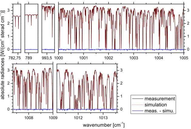
64 M. Schneider and F. Hase: Monitoring total ozone with a precision of around 1 DU 782,75 0 1 2 3 789 993,5 1000 1001 1002 1003 1004 1005 0 1 2 3 1008 1009 0 1 2 3 1012 1013 0 1 2 3 a b s o l u t e r a d i a n ce s [ W / ( c m 2 st e r a d cm -1 ) ] wavenumber [cm -1 ] measurement simulation meas. - simu.
Fig. 1. Spectral windows applied. Plotted is the situation for a real measurement taken on 22nd of January 2005 (solar elevation angle
32.2◦); black line: measured spectrum; red line: simulated spectrum; blue line: difference between simulation and measurement.
for the a-priori knowledge: Sais the a-priori covariance
ma-trix and xa represents the a-priori state. We apply the
inver-sion code PROFFIT (Hase et al., 2004) which uses the Karl-sruhe Optimised and Precise Radiative Transfer Algorithm (KOPRA, H¨opfner et al., 1998; Kuntz et al., 1998; Stiller et al., 1998) as forward model.
We use spectral microwindows with48O3and
asymmet-ric and symmetasymmet-ric50O3 and49O3 absorption signatures in
the mid-infrared (between 780–1015 cm−1; see Fig. 1). In the 782.75 and 789.0 cm−1windows only the main isotopo-logue (48O3) has absorption signatures. There are also minor
interferences from CO2, H2O, and solar lines. These two
mi-crowindows are the same that were used in Schneider et al. (2005). The strongest line in the 993.5 cm−1 window is a symmetric50O3signature (at 993.8 cm−1). Other signatures
are from48O3, asymmetric50O3, symmetric and asymmetric 49O
3, H2O, CO2, and solar lines. Broadband microwindows
are very useful to improve the sensitivity of the observing system for the lower troposphere (Barret et al., 2002). We apply three broadband microwindows between 1000.0 and 1013.6 cm−1. In these microwindows all 48O3, 50O3, and 49O
3isotopologues have absorption signatures. The main
in-terfering species are H2O and CO2.
We make an OE of48O3, asymmetric, and symmetric50O3
and of the isotopologue ratio profiles of48O3/50O3. The
lat-ter is an option recently introduced in PROFFIT (Schneider
et al., 2006), which provides for an improved constraint of the resulting profiles. As a-priori of O3(mean profile and
co-variances) we use a climatology of Iza˜na’s ECC-sondes from 1996 to 2006. However, in this and the following section we show that the choice of the a-priori is a minor error source and consequently our conclusions are not limited to Iza˜na. As a-priori for the typical ozone isotopologue ratio profiles and their covariances we use data reported by Johnson et al. (2000). The spectral signatures of the minor isotopologues of
49O
3are only considered by scaling a climatological profile.
The H2O interferences are considered by scaling an actual
H2O profile as retrieved in a previous step from specific H2O
microwindows of the same measurement. This H2O retrieval
is described in Schneider et al. (2006). The minor signatures of CO2 and C2H4are considered by scaling corresponding
climatological profiles.
The applied temperature data are a combination of the data from the local ptu-sondes (up to 30 km) and data supplied by the automailer system of the Goddard Space Flight Cen-ter. The spectroscopic line parameters of H2O and of O3
are taken from the HITRAN 2004 database (Rothman et al., 2005). For all other species we apply HITRAN 2000 pa-rameters (Rothman et al., 2003). To minimise errors due to uncertainties of the instrumental line shape we monitor and eventually correct line shape distortions regularly ev-ery two months. These measurements consist in independent
et al. (1999). The σ of Eq. (1) is taken from the residuals of the fit itself, performing an automatic adjustment of the constraints according to the noise level found in each mea-surement.
2.2 Error estimation
Our error analysis bases on the analytic method suggested by Rodgers (2000), where the difference between the retrieved and the real state (ˆx−x) — the error — is linearised about a mean profile xa, the estimated model parameterspˆ, and the
measurement noise ǫ:
ˆx−x =
( ˆA−I)(x−xa)
+ ˆG ˆKp(p− ˆp)
+ ˆGǫ (2)
Here I is the identity matrix, ˆA the averaging kernel matrix,
ˆ
G the gain matrix, and ˆKp a sensitivity matrix to model
pa-rameters. Equation (2) identifies the three classes of errors. These are: (a) errors due to the inherent finite vertical reso-lution of the observing system (smoothing error), (b) errors due to uncertainties in the input parameters applied in the in-version procedure, and (c) errors due to measurement noise (with standard deviation ǫ).
Generally one assumes linearity of the forward model within the range of the variability of the atmospheric state. Then the errors are calculated according to Eq. (2) applying single mean matrices for ˆA, ˆG, and ˆKp. However, for the
saturated (or nearly saturated) spectral O3lines as shown in
Fig. 1 the Jacobians depend on the actual atmospheric state. Therefore, we use an ensemble of 500 real states which obeys the a-priori statistics and calculate for each individual mem-bers of this ensemble the matrices ˆA, ˆG, and ˆKp: we make
for each of the 500 real states an individual error estimation according to Eq. (2).
An error estimation should distinguish systematic and ran-dom errors. Generally one defines the global mean and stan-dard deviation of a large ensemble of errors as the systematic and the random error component. However, this global trement disregards that the errors may depend on the actual at-mospheric state or the observing geometry. For example, an error may depend on the actual atmospheric O3distribution:
an optimal estimation approach constrains towards a clima-tological a-priori amount. This constraint favours positive errors in O3amounts below the a-priori amount and negative
errors in O3amounts above the a-priori amount. In this
sec-tion we examine the dependence of the errors on the total O3
amounts. In addition an error may depend on the strength of the absorption signal. This strength is determined by the O3
slant column amount, i.e. by a combination of the actual O3
distribution and the observing geometry. In Sect. 3 we show how the errors depend on the O3slant column amounts.
3
separate the random and systematic errors by means of a least squares fit. The regression curve of a least squares fit gives the systematic error, i.e. it documents how the observ-ing system as a mean reflects the real atmospheric situation. It seems sufficient to apply linear least squares fits. One sys-tematic error is the difference of the slope of the regression line from zero. It shows how the observing system systemat-ically under- or overestimates the real variabilities. We call this error “sensitivity error”. It is significant for uncertain-ties in the temperature profiles and the line parameters (for more details see Sect. 2.2.2). Another systematic error com-ponent can be seen as an offset of the regression line. This ’bias error’ is due to systematic error sources or incorrect a-priori assumptions. The values we give as bias error refer to the offset of the regression line at the a-priori value (cli-matological value). It is in particular large for errors due to intensity offsets, uncertainties in the temperature profile, and uncertainties in the line intensities. The scattering around the regression line gives the random error. The correlation coef-ficient of the linear least squares fit is linked to the scattering around the regression line (e.g. Wilks, 1995):
σǫreg= σǫ
q
1 − ρ2 (3)
Here σǫregis the scattering around the regression line, i.e. the
random error component, σǫ is the scattering of the
ensem-ble values, and ρ the correlation coefficient. For more de-tails about this method of error calculations please consult Schneider et al. (2006).
2.2.1 Smoothing error
According to Eq. (2) the smoothing error is given by
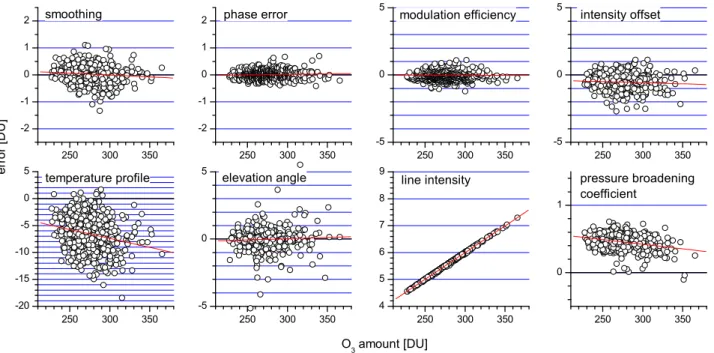
( ˆA−I)(x−xa). The upper left panel of Fig. 2 shows the cor-relation between O3amount and the smoothing error. The
smoothing error has no systematic bias error component (no offset at the priori value). This is trivial, since we use as a-priori the same statistics that was applied for the simulation of the ensemble profiles. However, it is not trivial that there is nearly no systematic sensitivity error (slope of regression line of 0.998). This nearly perfect sensitivity demonstrates that the choice of the a-priori has a negligible impact on the retrieved O3amounts. The random error component is
0.36 DU. The estimated systematic and random smoothing errors are listed together with the other errors in Table 2. 2.2.2 Input parameter errors
In this subsection errors due to uncertainties in solar an-gle, instrumental line shape (ILS: modulation efficiency and phase error Hase et al., 1999), baseline of the spectrum (in-tensity offset), temperature profile, and spectroscopic param-eters (line intensity and pressure broadening coefficient) are estimated. The assumed parameter uncertainties (p− ˆp)are
66 M. Schneider and F. Hase: Monitoring total ozone with a precision of around 1 DU 250 300 350 -2 -1 0 1 2 250 300 350 -2 -1 0 1 2 250 300 350 -5 0 5 250 300 350 -5 0 5 250 300 350 -20 -15 -10 -5 0 5 250 300 350 -5 0 5 250 300 350 4 5 6 7 8 9 250 300 350 0 1 e r r o r [ D U ]
smoothi ng phase error modul ati on effi ci ency i ntensi ty offset
temperature profi l e el evati on angl e
O 3
amount [DU]
l i ne i ntensi ty pressure broadeni ng coeffi ci ent
Fig. 2. Errors of retrieved total O3 amounts versus total O3amounts. Circles represent the 500 individual members of the applied ensemble.
The red lines are the linear regression lines. The blue griding is the same in every panel and helpful to identify the relative importance of the error.
Table 1. Assumed uncertainties.
error source random systematic phase error 0.01 rad – modulation eff. 1 % – intensity offset 0.1 % +0.1 % T profile at surface 1.7 K −3.5 K rest of troposphere 0.7 K – at 30 km 1 K up to +4 K above 50 km 6 K up to −12 K solar angle 0.1◦ – line intensity – −2 %
pres. broad. coef. – −2 %
αdetailed description see text
We estimate the ILS stability from regularly performed low pressure N2O cell measurements (Hase et al., 1999), to
0.01 rad for the phase error and 1% for the modulation effi-ciency. An intensity offset may be caused by detector non-linearities. Here we use a photo-voltaic MCT detector in-stead of the usually applied photo-conductive detectors. It has the advantage of reduced non-linearities and thus an im-proved zero baseline determination (less spectral intensity offset). We estimate the spectral intensity offset in our spec-tra by analysing very intense O3signatures between 1024.25
and 1025 cm−1. Those signatures are saturated even for O3
slant columns as low as 250 DU. We found a mean offset
of 0.1 % and a standard deviation of 0.1 % in the core of the saturated lines. Two sources are considered as random uncer-tainty in the temperature profile: first, the measurement un-certainty of the sonde, which is assumed to be 0.5 K through-out the whole troposphere and to have no interlevel correla-tions. Second, the temporal differences between the FTIR and the sonde’s temperature measurements, which are esti-mated to be 1.5 K at the surface and 0.5 K in the rest of the troposphere, with a correlation length of 5 km. Furthermore, we assume systematic errors in the temperature profile (for more details please see Sect. 3).
The parameter errors are calculated according to Eq. (2) by ˆG ˆKp(p− ˆp). Subsequently we estimate their systematic
and random components by correlation to the O3 amounts.
The correlations are shown in Fig. 2. The systematic and random errors are estimated as for the smoothing error: from the slope and bias of the regression line and the correlation coefficient (see Eq. 3). The assumed uncertainties of Table 1 lead to large random and systematic errors due to uncertain-ties in the temperature profile (random: 3.5 DU; sensitivity error: −3.3 %; bias: −7.0 DU). We also made these simu-lation assuming no systematic error in the temperature pro-file, i.e. assuming no error for the temperature dependence of the pressure broadening coefficient. In this case the random error remains unchanged at 3.5 DU, but the systematic com-ponents reduce significantly: to −1.6 % for the sensitivity error and to −0.2 DU for the bias. Although reduced, there is still a systematic sensitivity error even in the absence of a systematic temperature error source.
solar elevation angle, and modulation efficiency (0.4, 0.3 and 0.3 DU, respectively). All other random errors are negligible, i.e. are situated below 0.2 DU. Significant systematic errors are produced by errors in the line intensity parameter (error of 2 % column amount error for 2 % parameter error) and due to an intensity offset (error of −0.2 % for assumed systematic offset of 0.1 %). A systematic error in the pressure broaden-ing coefficient causes only very small systematic errors in the column amounts. All errors are collected in Table 2. 2.2.3 Measurement noise error
This error is due to statistical fluctuation in the measured sig-nal, caused by e.g. photon noise or thermal noise in the detec-tor or noise produced by the signal amplification. It causes white noise in the residuals. With the Bruker IFS 125HR and the applied photo-voltaic MCT detector we reach a signal to noise ratio of typically 1000 around 1000 cm−1. We found this value by analysing measured spectra in regions with no absorption issues. Its impact on total column amounts is neg-ligible. Our simulations lead to errors below 0.1 DU (see Table 2).
3 Simultaneous optimal estimation of O3and
tempera-ture profiles
Table 2 reveals that uncertainties in the assumed temperature profile are mainly responsible for the overall errors in the retrieved columns amounts. Both the shape and the area of an absorption line depend on the temperature. Thus, errors in the temperature profile lead to erroneous simulations of the line shapes and areas and consequently to errors in the retrieved trace gas profiles.
The applied inversion code PROFFIT allows a joint op-timal estimation of temperature profile together with VMR profiles. From the viewpoint of the forward model, the re-trieval of temperature brings in several complications: the absorption cross sections cannot be precomputed before the iterative retrieval process is performed, instead recalculation in each iteration step is required. Derivatives of tempera-ture have to be provided at each model level. The construc-tion of the temperature derivatives within the forward model KOPRA used here, is described in Stiller et al. (2000). Fi-nally, as hydrostatic equilibrium is assumed, it has to be taken into account that a change of the temperature profile impli-cates a modified pressure stratification. Therefore, in each iteration step an atmosphere in hydrostatic balance is recon-structed and the pressure at each altitude fixed model level is changed according to the current temperature profile. From the viewpoint of the retrieval, the joint fit of temperature re-quires extensions to the state vectors, the Jacobian and the a-priori covariances. An a-priori temperature profile and as-sociated a-priori covariance have to be provided by the user
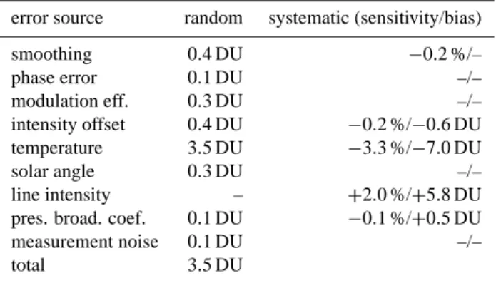
Table 2. Estimated random (in DU) and systematic errors
(sensi-tivity in % and bias in DU) of the total column amounts.
error source random systematic (sensitivity/bias) smoothing 0.4 DU −0.2 %/– phase error 0.1 DU –/– modulation eff. 0.3 DU –/– intensity offset 0.4 DU −0.2 %/−0.6 DU temperature 3.5 DU −3.3 %/−7.0 DU solar angle 0.3 DU –/– line intensity – +2.0 %/+5.8 DU
pres. broad. coef. 0.1 DU −0.1 %/+0.5 DU
measurement noise 0.1 DU –/– total 3.5 DU
as additional input. The a-priori temperature profiles used here are a combination of the daily ptu-sonde and the God-dard NCEP temperatures as described in Sect. 2. The a-priori temperature covariance is constructed in accordance with the assumed random error budget of the temperature profile (see Table 1). The reasons for the random temperature errors have been discussed in Sect. 2. We also found systematic differ-ences between our optimally estimated temperature profiles and the ptu-sonde/NCEP temperature profiles, which we in-terpret as systematic temperature errors. There are several reasons for these systematic differences: (a) the ptu-sonde is released at sea level. It already measures the temperature of the free troposphere when reaching the altitude of FTIR mountain site. In the free troposphere the temperature is gen-erally lower than at the FTIR site. (b) At higher altitudes the sonde may give to large temperatures due to radiative heating (c) The Goddard NCEP temperatures may have systematic errors. (d) The parameterisation of the temperature depen-dence of the O3 line width may be erroneous. Such a
sys-tematic error in the spectroscopic data produces syssys-tematic differences between actual and retrieved temperature profile. We analyse how a joint optimal estimation of the tempera-ture profiles reduces the impact of temperatempera-ture uncertainties on the retrieved O3 column amounts. We calculate for all
500 members of the ensemble the matrices ˆA, ˆG, and ˆKpfor
the new retrieval setup and perform the same error simula-tion as in Sect. 2. We found that an OE estimasimula-tion of the temperature applying the O3 windows of Fig. 1 already
re-duces the temperature error. However, an additional applica-tion of CO2windows should allow for further improvements.
Spectral signatures of CO2are often used in remote sensing
to determine temperature profiles. Atmospheric CO2is very
stable. It has little temporal variability and its mixing ra-tios are nearly constant over large altitude regions. Changes in the CO2absorption pattern can thus be mainly attributed
68 M. Schneider and F. Hase: Monitoring total ozone with a precision of around 1 DU 963 0 1 2 3 965 968 969 0 1 2 3 a b so l u t e r a d i a n ce s [ W / ( c m 2 st e r a d cm -1 ) ] wavenumber [cm -1 ] measurement simulation meas. - simu.
Fig. 3. Applied CO2windows. The spectra correspond to the same measurement as the spectra shown in Fig. 1. Scale and meaning of lines
and colours is the same as in Fig. 1
Table 3. Estimated random (in DU) and systematic errors (in %)
of O3total column amounts for simultaneous optimal estimation of
O3and temperature profiles.
error source random systematic (sensitivity/bias) smoothing 0.5 DU –/– phase error 0.3 DU –/– modulation eff. 0.7 DU +0.1 %/– intensity offset 0.6 DU +0.3 %/−0.9 DU temperature 0.1 DU −0.2 %/−0.4 DU solar angle 0.3 DU –/– line intensity – +2.0 %/+5.7 DU
pres. broad. coef. 0.1 DU −0.1 %/+0.3 DU
measurement noise 0.1 DU –/– total 1.2 DU
an infrared active gas and its concentrations are relatively high which assures distinct absorption signatures. We ap-ply four spectral windows between 960 and 970 cm−1 con-taining isolated CO2lines of different intensities (see Fig. 3)
together with the windows as described in Sect. 2 and shown in Fig. 1. The only significantly interfering absorptions in the CO2windows are due to O3and can be seen as the tiny
dips in the 969 cm−1window. To adjust the measured and simulated CO2signatures we only allow a scaling of a
cli-matological CO2profile. The remaining observed residuals
contain the information about the actual temperature profile. For this retrieval setup the errors due to temperature uncer-tainties are widely eliminated. The random error is reduced from 3.5 DU to 0.1 DU. The systematic sensitivity error is re-duced from −3.3 % to −0.2 % and the systematic bias from
−7.0 DU to −0.4 DU. The smoothing error, the intensity
off-set, and errors due to uncertainties in the ILS and the solar elevation angle remain as leading error sources. Following the assumptions listed in Table 1 we estimate a total random error of around 1.2 DU. This is a significant improvement
over the current state-of-the-art retrieval method for which we estimate a total random error of 3.5 DU. All errors are listed in Table 3.
In Sect. 2 is has been shown how the errors typically de-pend on the total O3amounts. In this section we examine the
dependence on the O3absorption signature. The O3
absorp-tion signature is determined by the O3slant column amount.
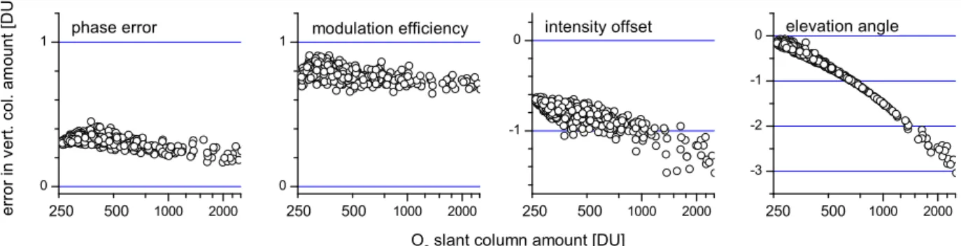
Figure 4 shows the dependence of the errors for a simulta-neous OE of O3 and temperature. It is in particular strong
for the solar elevation error. For high slant column amounts, i.e. low elevation angle, a small uncertainty of 0.1◦produces errors of larger than 2 DU, whereas for low slant column amounts (or large elevation angles) these errors are below 0.2 DU. Vice versa errors due to an incorrect pressure broad-ening coefficient or due to uncertainties in the phase error are larger at low slant column amounts than at large slant column amounts.
Current FTIR systems are very stable experiments. Small, undetected ILS distortions or solar tracker misalignments may maintain constant over several months and are conse-quently systematic error sources. In Fig. 5 we characterise the errors produced by systematic uncertainties in the phase error, the modulation efficiency, the intensity offset, and the solar angle. For the modulation efficiency and the phase error we assume a systematic uncertainty of −1 % and +0.01 rad, respectively. For the intensity offset and the temperature pro-file we use the systematic uncertainties as listed in Table 1. This analysis completes our error characterisation. It shows that the errors produced by uncertainties in the phase error are slightly larger for low slant column amounts than for large slant column amounts: at 400 DU the errors are 0.4 DU and above 1000 DU the errors are close to 0.2 DU. A similar dependence can be observed for errors due to uncertainties in the modulation efficiency. By contrast the errors due to an intensity offset or a misalignment of the solar tracker are larger at large slant column amounts than at low slant column amounts.
1000 2000 -2 -1 0 1 2 1000 2000 -2 -1 0 1 2 1000 2000 -5 0 5 1000 2000 -5 0 5 1000 2000 -1 0 1 1000 2000 -5 0 5 1000 2000 4 5 6 7 8 9 1000 2000 0 1 e r r o r i n v e r t i c a l c o l u m n a m o u n t [ D U ]
smoothi ng phase error modul ati on effi ci ency i ntensi ty offset
temperature profi l e 250 500 250 500 250 500 250 500 250 500 250 500 250 500 el evati on angl e O 3
sl ant col umn amount [DU] 250 500
l i ne i ntensi ty pressure broadeni ng coeffi ci ent 1000 2000 0 1 1000 2000 0 1 1000 2000 -1 0 1000 2000 -3 -2 -1 0 e r r o r i n v e r t . c o l . a m o u n t [ D U ]
phase error modul ati on effi ci ency i ntensi ty offset
250 500 250 500 250 500 250 500 el evati on angl e O 3
sl ant col umn amount [DU]
Fig. 4. Same as Fig. 2 but for new retrieval approach (i.e. simultaneous optimal estimation of O3and temperature profiles) and versus O3
slant column amounts (error assumptions according to Table 1).
1000 2000 -2 -1 0 1 2 1000 2000 -2 -1 0 1 2 1000 2000 -5 0 5 1000 2000 -5 0 5 1000 2000 -1 0 1 1000 2000 -5 0 5 1000 2000 4 5 6 7 8 9 1000 2000 0 1 e r r o r i n v e r t i c a l c o l u m n a m o u n t [ D U ]
smoothi ng phase error modul ati on effi ci ency i ntensi ty offset
temperature profi l e 250 500 250 500 250 500 250 500 250 500 250 500 250 500 el evati on angl e O 3
sl ant col umn amount [DU] 250 500
l i ne i ntensi ty pressure broadeni ng coeffi ci ent 1000 2000 0 1 1000 2000 0 1 1000 2000 -1 0 1000 2000 -3 -2 -1 0 e r r o r i n v e r t . c o l . a m o u n t [ D U ]
phase error modul ati on effi ci ency i ntensi ty offset
250 500 250 500 250 500 250 500 el evati on angl e O 3
sl ant col umn amount [DU]
Fig. 5. Same as Fig. 4, but for only systematic error sources. 4 Summary and conclusions
Applying a state-of-the-art instrumentation and retrieval strategy provides for an estimated precision of total O3 of
around 1DU, which converts the FTIR technique to one of the most precise techniques for a continuous monitoring of total O3. From Table 3 we conclude that important
remain-ing error sources are intensity offsets, small uncertainties of the ILS or of the solar elevation angle, and the smoothing er-ror. It is, furthermore, important to state that we estimate a near ideal column sensitivity. Therefore, the applied a-priori has negligible influence on the retrieved O3 amounts. All
information about the actual O3 content is taken from the
measurement and in consequence our error estimation is of general validity and not limited to the Iza˜na site. The recipe is summarized as follows and contains retrieval and instru-mental aspects:
(1) To eliminate the temperature error and to keep the smoothing error small it is required to apply the retrieval strategy described in the previous sections, i.e. it is manda-tory to apply broad spectral windows, to perform a joint OE of48O3,48O3/50O3, and of the temperature profiles. to
opti-mise the temperature retrieval one should introduce the spec-tral CO2 windows as shown in Fig. 3. The joint OE of the
temperature profile provides for the decisive improvement of the precision. Currently PROFFIT (Hase et al., 2004) is the only retrieval code for the analysis of ground-based spectra that allows to perform an OE of temperature and isotopo-logue profiles.
(2) One should apply a voltaic instead of a photo-conductive detector. Photo-voltaic detectors have a quite lin-ear characteristics whereas photo-conductive detectors show a certain level of non-linearity, which may offset the zero baseline of the measured spectra.
70 M. Schneider and F. Hase: Monitoring total ozone with a precision of around 1 DU (3) One should use an instrument with a stable ILS like the
Bruker IFS 120/125HR. Currently the Bruker IFS 120/125 HR spectrometers are among the best-performing FTIR spec-trometers commercially available. It is difficult to achieve the required stability with portable instruments like a Bruker IFS 120M.
(4) The pointing of the solar tracker and the effective mea-surement time should be known with high accuracy. For a so-lar elevation angle of 45◦an uncertainty of 0.1◦in the point-ing or of 30 s in the effective measurement time causes an error of 0.3 DU. For an elevation angle of 20◦ or 10◦ this error increases to 1.3 DU and 2.2 DU, respectively. At Iza˜na we apply a high quality home-built solar tracker. Its mirror positions are determined from astronomical calculations and additionally controlled by the signals of a quadrant detector (Huster, 1998).
(5) The intensity fluctuations during scanning should be documented. For example, clouds passing through the line of sight during scanning may cause intensity offsets in the spectra. A correction of these baseline artefacts is only pos-sible if in addition to the AC interferogram signal the DC interferogram signal is recorded. At Iza˜na such a correction was not necessary due to the nearly continuous perfect clear sky conditions, however at sites with less favorable sky con-ditions it is indispensable.
Finally, it should be commented that a further reduction of the noise level would yield no further improvement: as shown in Table 3 the measurement noise is a negligible error source.
Acknowledgements. We would like to thank the European
Commission for funding via the project GEOMON (contract GEOMON-036677). Furthermore, we are grateful to the Goddard Space Flight Center for providing the temperature and pressure profiles of the National Centers for Environmental Prediction via the automailer system.
Edited by: A. Hofzumahaus
References
Barret, B., De Mazi`ere, M., and Demoulin, P.: Retrieval and char-acterization of ozone profiles from solar infrared spectra at the Jungfraujoch, J. Geophys. Res, 107, 4788–4803, 2002.
De Mazi`ere, M., Barret, B., Vigouroux., C., Blumenstock, T., Hase, F., Kramer, I., Camy-Peyret, C., Chelin, P., Gardiner, T., Coleman, M., Woods, P., Ellingsen, K., Gauss, M., Isaksen, I., Mahieu, E., Demoulin, P., Duchatelet, P., Mellqvist, J., Strand-berg, A., Velazco, V., Schulz, A., Notholt, J., Sussmann, R., Stremme, W., and Rockmann, A.: Ground-based FTIR measure-ments of O3and climate related gases in the free troposphere
and lower stratosphere, presented at the Quadrenial Ozone Sym-posium, 529, Kos, Greece, 2004.
Hase, F., Blumenstock, T., and Paton-Walsh, C.: Analysis of the instrumental line shape of high-resolution Fourier transform IR
spectrometers with gas cell measurements and new retrieval soft-ware, Appl. Opt., 38, 3417–3422, 1999.
Hase, F., Hannigan, J. W., Coffey, M. T., Goldman, A., H¨opfner, M., Jones, N. B., Rinsland, C. P., and Wood, S. W.: Intercompar-ison of retrieval codes used for the analysis of high-resolution, ground-based FTIR measurements, J. Quant. Spectrosc. Ra., 87, 25–52, 2004.
H¨opfner, M., Stiller, G. P., Kuntz, M., Clarmann, T. v., Echle, G., Funke, B., Glatthor, N., Hase, F., Kemnitzer, H., and Zorn, S.: The Karlsruhe optimized and precise radiative transfer algo-rithm, Part II: Interface to retrieval applications, SPIE Proceed-ings 1998, 3501, 186–195, 1998.
Huster, S. M.: Bau eines automatischen Sonnenverfolgers f¨ur bo-dengebundene IR-Absorptionmessungen, Diplomarbeit im Fach Physik, Institut f¨ur Meteorologie und Klimaforschung, Univer-sit¨at Karlsruhe und Forschungszentrum Karlsruhe, 1998. Johnson, D. G., Jucks, K. W., Traub, W. A., and Chance, K. V.:
Isotopic composition of stratospheric ozone, J. Geophys. Res., 105, 9025–9031, 2000.
Kuntz, M., H¨opfner, M., Stiller, G. P., Clarmann, T. v., Echle, G., Funke, B., Glatthor, N., Hase, F., Kemnitzer, H., and Zorn, S.: The Karlsruhe optimized and precise radiative transfer algorithm, Part III: ADDLIN and TRANSF algorithms for modeling spec-tral transmittance and radiance, SPIE Proceedings 1998, 3501, 247–256, 1998.
Rodgers, C. D.: Inverse Methods for Atmospheric Sounding: The-ory and Praxis, World Scientific Publishing Co., Singapore, ISBN 981-02-2740-X, 2000.
Rothman, L. S., Barbe, A., Benner, D. C., Brown, L. R., Camy-Peyret, C., Carleer, M. R., Chance, K. V., Clerbaux, C., Dana, V., Devi, V. M., Fayt, A., Fischer, J., Flaud, J.-M., Gamache, R. R., Goldman, A., Jacquemart, D., Jucks, K. W., Lafferty, W. J., Mandin, J.-Y., Massie, S. T., Newnham, D. A., Perrin, A., Rins-land, C. P., Schroeder, J., Smith, K. M., Smith, M. A. H., Tang, K., Toth, R. A., Vander Auwera, J., Varanasi, P., and Yoshino, K.: The HITRAN Molecular Spectroscopic Database: Edition of 2000 Including Updates through 2001, J. Quant. Spectrosc. Ra., 82, 5–44, 2003.
Rothman, L. S., Jacquemart, D., Barbe, A., Benner, D. C., Birk, M., Brown, L. R., Carleer, M. R., Chackerian Jr., C., Chance, K. V., Coudert, L. H., Dana, V., Devi, J., Flaud, J.-M., Gamache, R. R., Goldman, A., Hartmann, J.-M., Jucks, K. W., Maki, A. G., Mandin, J.-Y., Massie, S. T., Orphal, J., Perrin, A., Rinsland, C. P., Smith, M. A. H., Tennyson, J., Tolchenov, R. N., Toth, R. A., Vander Auwera, J., Varanasi, P., and Wagner, G.: The HI-TRAN 2004 molecular spectroscopic database, J. Quant. Spec-trosc. Ra., 96, 139–204, 2005.
Schneider M., Blumenstock, T., Hase, F., H¨opfner, M., Cuevas, E., Redondas, A., and Sancho, J. M.: Ozone profiles and total col-umn amounts derived at Iza˜na, Tenerife Island, from FTIR solar absorption spectra, and its validation by an intercomparison to ECC-sonde and Brewer spectrometer measurements, J. Quant. Spectrosc. Ra., 91, 245–274, 2005.
Schneider, M., Hase, F., and Blumenstock, T.: Ground-based re-mote sensing of HDO/H2O ratio profiles: introduction and vali-dation of an innovative retrieval approach, Atmos. Chem. Phys., 6, 4705–4722, 2006,
http://www.atmos-chem-phys.net/6/4705/2006/.
Stiller, G. P., H¨opfner, M., Kuntz, M., Clarmann, T. v., Echle, G.,
Zorn, S.: The Karlsruhe optimized and precise radiative trans-fer algorithm, Part I: Requirements, justification and model error estimation, SPIE Proceedings 1998, 3501, 257–268, 1998. Stiller, G. P., Clarmann, T. v., A. Dudhia, G. Echle, B. Funke,
N. Glatthor, F. Hase, M. Hpfner, S. Kellmann, H. Kem-nitzer, M. Kuntz, A. Linden, M. Linder, G. P. Stiller, and S. Zorn: The Karlsruhe Optimized and Precise Radiative trans-fer Algorithm (KOPRA), Forschungszentrum Karlsruhe, Wis-senschaftliche Berichte, Bericht Nr. 6487, 2000.
recovery of the ozone layer, Nature, 441, 39–45, 2006.
Wilks, D. S.: Statistical methods in the atmospheric science, Aca-demic Press, ISBN 0-12-751965-3, 1995.