HAL Id: hal-01398972
https://hal.archives-ouvertes.fr/hal-01398972
Submitted on 18 Nov 2016
HAL is a multi-disciplinary open access archive for the deposit and dissemination of sci-entific research documents, whether they are pub-lished or not. The documents may come from teaching and research institutions in France or
L’archive ouverte pluridisciplinaire HAL, est destinée au dépôt et à la diffusion de documents scientifiques de niveau recherche, publiés ou non, émanant des établissements d’enseignement et de recherche français ou étrangers, des laboratoires
From tree-decompositions to clique-width terms
Bruno Courcelle
To cite this version:
Bruno Courcelle. From tree-decompositions to clique-width terms. Discrete Applied Mathematics, Elsevier, 2018. �hal-01398972�
From tree-decompositions to clique-width terms
Bruno Courcelle
Labri, CNRS and Bordeaux University
∗33405 Talence, France
email: [email protected]
June 9, 2016
Abstract
Tree-width and clique-width are two important graph complexity mea-sures that serve as parameters in many fixed-parameter tractable algo-rithms. We give two algorithms that transform tree-decompositions rep-resented by normal trees into clique-width terms. As a consequence, we obtain that for sparse graphs, clique-width is polynomially bounded in terms of tree-width. It is even linearly bounded for planar graphs and incidence graphs. These results have applications to model-checking algo-rithms for problems described by monadic second-order formulas, includ-ing those allowinclud-ing edge set quantifications.
Introduction
Tree-width and clique-width are important graph complexity measures that oc-cur as parameters in many fixed-parameter tractable (FPT) algorithms [12, 14, 16, 17, 21]. They are also important for the study of graph structure and, in particular, for the description of certain graph classes by forbidden subgraphs, minors or vertex-minors. Both notions are based on certain hierarchical graph decompositions, and the associated FPT algorithms use dynamic programming on these decompositions. Many of these algorithms need input graphs of moder-ate tree-width or clique-width that are given with the relevant decompositions. Constructing optimal decompositions is difficult [1, 20], however, there exist polynomial time approximation algorithms [2, 27].
A related problem consists in comparing width measures in the following way. Given two width measures wd and wd′ and a graph class C, we wish to prove
∗This work has been supported by the French National Research Agency (ANR) within
the IdEx Bordeaux program "Investments for the future", CPU, ANR-10-IDEX-03-02, and also within the project GraphEn started in October 2015. Parts of it have been presented to a worshop on graph decompositions at CIRM (Marseille, France) in January 2015.
that wd′(G) ≤ f(wd(G)) for every graph G in C, where f is a fixed function.
We say that wd′is linearly bounded (resp. polynomially bounded) in terms of wd
on C, if f is linear (resp. polynomial). In view of algorithmic applications, it is also useful to have efficient algorithms to convert a decomposition witnessing wd(G) ≤ k into one witnessing wd′(G) ≤ f (k).
For the class of all graphs, clique-width1 is not polynomially bounded in
terms of tree-width [5], and tree-width is not bounded in terms of clique-width by any function. For several classes of sparse graphs (these graphs have O(n) edges for n vertices, see Section 1), clique-width is polynomially bounded in terms of tree-width, and even linearly bounded for planar graphs, graphs of bounded degree and incidence graphs. In this article, we improve some known bounds, we obtain bounds for directed graphs and we give an algorithm that transforms tree-decompositions into clique-width terms. Together with combinatorial lemmas relative to each considered class, this algorithm yields the claimed linear or polynomial bounds. In the same framework, we present the algorithm from [5] that gives a better exponential bounding for graphs of large clique-width.
Our algorithms take as input a tree-decomposition represented in a compact way by a normal tree, i.e., a rooted tree such that the nodes of the tree are the vertices of the graph and adjacent vertices are comparable with respect to the ancestor relation of the tree. This representation is easier to implement (and perhaps also to visualize, but this is a subjective matter) than the pair (T, f) of the classical definition. It works well for our algorithms and offers also an easy logical representation (as observed in [12], Example 5.2(4)). Normal trees fit well with edge contractions and vertex and edge deletions, the transformations from which the quasi-order of minor inclusion is defined.
The actual input of our algorithms is a normal tree : the associated tree-decomposition is not necessary. It can be obtained from the algorithm as a by-product.
We also give a definition of clique-width that relaxes constraints on the use of vertex labels and facilitates the construction of clique-width terms. These constructions have been implemented (see Section 6).
Many model-checking algorithms for tree-structured graphs (graphs of boun-ded tree-width, path-with, clique-width, etc.) use dynamic programming on terms or labelled trees that encode the relevant decompositions. In several articles [9, 11], we construct FPT algorithms parameterized by clique-width for problems expressed in monadic second-order logic (MSO logic in short); these algorithms are based on fly-automata2taking clique-width terms as inputs.
MSO formulas using edge set quantifications (called simply MSO2 formulas)
are more expressive than MSO formulas. However, the MSO2 properties of a
1Clique-width is defined algebraically from terms that define graphs. Such terms are called
width terms, see Definition 3. An alternative definition is in [13]. We denote the clique-width of a graph G by cwd(G) and its tree-clique-width by twd(G).
2The finite automata arising from MSO formulas are much too large to be implemented in
the usual way by lists of transitions. In fly-automata, states and transitions are not tabulated but described by means of an appropriate syntax. Each time a transition is necessary, it is (re)computed. Only the transitions necessary for a given term are computed.
graph G are nothing but MSO properties of its incidence graph Inc(G). As the clique-width of Inc(G) is linearly bounded in terms of the tree-width of G, the algorithms for the MSO model-checking of graphs of bounded clique-width can be used (in practice) for the MSO2 model-checking of graphs of bounded
tree-width. This extension is developped in [7, 8].
Summary and main results.
Section 1 reviews notation about trees and graphs. Section 2 defines our novel presentations of tree-decompositions and clique-width terms. Section 3 presents in a unified way three algorithms that convert tree-decompositions into clique-width terms. In Section 4, we obtain that cwd(G) = O(twd(G)) for planar graphs (we improve the linear bound given in [22]) and that cwd(G) = O(twd(G)q) for uniformly q-sparse graphs (the graphs whose subgraphs have at
most qn edges for n vertices). In Section 5, we consider q-hypergraphs (their hyperedges have at most q vertices). A q-hypergraph H can be viewed as a bipartite graph Bip(H) and we prove that cwd(Bip(H)) = O(twd(H)q−1). For
incidence graphs, we deduce that cwd(Inc(G)) = O(twd(G)). In Section 6, we review the algorithmic applications to model-checking. In the appendix we consider the effect of minor-reducing operations on tree-decompositions defined by normal trees.
Acknowledgement: I thank I. Durand, S. Oum and M. Kanté for their useful comments.
1
Definitions and basic facts
Most definitions are well-known, we mainly review notation. We state a few facts that are either well-known or easy to prove.
The union of two disjoint sets is denoted by ⊎. The cardinality of a set X is denoted by |X| and its powerset by P(X).
If 0 ≤ m ≤ k, we define γ(k, m) as the number of subsets of [k] := {1, ..., k} of cardinality at most m. This number is 1 + k + ... + mk = O(km) for fixed
m. If 1 < m < k/2, then γ(k, m) < m mk < km/(m − 1)!. We will actually use
γ(k, m) for "small" fixed m and "large" variable k.
In this article, all trees, graphs and hypergraphs are nonempty and finite.
Trees
Trees are always rooted; NT denotes the set of nodes of a tree T and ≤T
its ancestor relation, a partial order on NT; the root, denoted by rootT, is the
unique maximal element and the leaves are the minimal ones; pT(u) is the father
(the closest ancestor) of a node u.
We denote by T≤(u) the set {w ∈ NT | w ≤T u}, by T<(u) the set {w ∈
If e is an edge of T between a node u and its father w, then the tree T′
resulting from the contraction of e is constructed as follows: we remove u and e and we make each son of u into a son of w. The root of T′ is that of T .
Graphs
Unless otherwise specified (as in Section 5.2), we consider simple graphs, i.e., they are loop-free and without parallel edges; they are directed or not. Undefined notions are as in [15]. A graph G has vertex set VGand edge set EG.
If G is directed, EG can be identified with the binary, irreflexive edge relation
edgG ⊆ VG× VG; while being simple, G can have pairs of opposite edges. If G is
undirected, then edgG is symmetric and |edgG| = 2 |EG| . The undirected graph
underlying G is Und(G) with VUnd(G):= VG and edgUnd(G):= edgG∪ edgG−1.
We denote by G[X] the induced subgraph of G with vertex set X ∩ VG. Note
that X need not be a subset of VG in order to deal easily with cases where X is
a set of vertices of a graph H of which G is a subgraph.
If G is directed and x ∈ VG, then NG+(x) is the set of vertices y such that
x →Gy (i.e., there is an edge from x to y), NG−(x) is the set of those such that
y →G x and NG(x) := NG+(x) ∪ NG−(x) is the set of neighbours of x. If G is
undirected, then NG(x) is the set of neighbours of x. We extend these definitions
to the case where x /∈ VG : then NG(x) = ∅. For a set3 X, NG+(X) is the union
of the sets NG+(x), x ∈ X, and similarly for NG and NG−.
If G is an undirected graph, and X, Y are disjoint sets, we define Ω(X, Y ) := {NG(x)∩Y | x ∈ X∩VG}; if G is directed, Ω(X, Y ) := {(NG+(x)∩Y, NG−(x)∩Y ) |
x ∈ X ∩ VG}. If G is undirected and Y is a set of vertices of G of cardinality k,
then |Ω(X, Y )| ≤ 2k. If furthermore 1 ≤ m ≤ k and |N
G(x)| ≤ m for all x ∈ X,
then |Ω(X, Y )| ≤ γ(k, m) = O(km) for fixed m. If G is directed, then each edge
of Und(G) between x and y can come from three possible configurations of edges between these vertices. Hence, if |Y | = k, we have |Ω(X, Y )| ≤ (1 + 3)k = 22k,
and if NUnd(G)(x) ≤ m ≤ k for all x ∈ X, we have |Ω(X, Y )| < 3mγ(k, m).
Sparse graphs
A graph G is uniformly q-sparse if |EH| ≤ q |VH| for every (undirected)
subgraph H of Und(G). An undirected graph G is uniformly q-sparse if and only if it has an orientation of indegree at most q ([23] or Proposition 9.40 of [12]). Every planar graph G is uniformly 3-sparse (because |EG| ≤ 3 |VG| − 6).
An undirected graph is uniformly ⌈d/2⌉-sparse if its maximum degree is d. We denote by Srthe class of graphs G such that Und(G) does not contain
a subgraph isomorphic to the complete bipartite graph Kr,r. These graphs are
Kr,r-free with respect to subgraph inclusion and removal of orientation. Every
uniformly q-sparse graph belongs to S2q+1, but for every r and q, there are
graphs in Srthat are not uniformly q-sparse (because there is a constant c such
that, if r ≥ 3, there is a graph having n vertices and at least c.n2−2/(r+1)edges,
see [15], Section 7.1).
3As for G[X], the set X need not be a subset of V
G. The same holds for X, Y in Ω(X, Y )
2
Tree-width and clique-width
2.1
Tree-decompositions of various kinds
Tree-decompositions are well-known, but we present new definitions concerning them.
Definitions 1: Normal trees and tree-decompositions.
(a) A tree T is quasi-normal for a graph G if VG⊆ NT and the two ends of
each edge of G are comparable under <T. It is normal if in addition, we have
VG = NT. A depth-first spanning tree of a graph is thus normal.
(b) In a tree-decomposition (T, f) of a graph G, the tree T is always rooted, f maps NT to P(VG) and satisfies the well-known conditions4. In cases where
VG ⊆ NT, we will denote by f∗(u) the set f (u) − {u}.
(c) A tree-decomposition (T, f ) of a graph G is normal (resp. quasi-normal ) if T is normal (resp. quasi-normal) for G and :
f (u) ⊆ T≥(u) for every u ∈ NT, and u ∈ f (u) for every node u of T
that is a vertex of G.
(d) Let a tree T be normal for a graph G. For each u ∈ VG, we define :
upG,T(u) := NG(u) ∩ T>(u),
up+G,T(u) := NG+(u) ∩ T>(u) and up−G,T(u) := NG−(u) ∩ T>(u) if G is
directed.
fT∗(u) := NG(T≤(u)) ∩ T>(u) = {upG,T(w) ∩ T>(u) | w ≤T u},
and finally,
fT(u) := {u} ∪ fT∗(u).
Hence, fT(u) consists of u and its ancestors that are adjacent to some vertex
w ≤T u.
If T is quasi-normal, we use the same notions and for u ∈ NT − VG, we
define :
fT(u) := fT∗(u).
We define the width of (G, T ) as the maximal cardinality of a set f∗ T(u).
Claim 1 : If T is quasi-normal (resp. normal) for a graph G, then (T, fT) is
a quasi-normal (resp. normal) tree-decomposition of this graph. The width of the tree-decomposition (T, fT) is that of (G, T ).
4that every vertex is in some bag f (u), every edge has its two ends in some bag, and the
connectivity condition holds : for every vertex, the nodes u such that f (u) contains it induce a connected subgraph of T .
Figure 1: A graph G and a normal tree T
Proof : We only check the connectivity condition, expressed here as follows : if y ∈ fT(u) ∩ fT(v), then u, v ≤T y and y belongs to each set fT(w) such that
u ≤T w ≤T y or v ≤T w ≤T y, hence, it belongs to each set fT(w) for w on the
undirected path between u and v. The other conditions obviously hold.
Claim 2 : If (T, f) is a quasi-normal tree decomposition, then fT(u) ⊆ f (u)
for all u.
Proof : Consider y ∈ fT(u). If y = u, then y ∈ f(u). Otherwise, x ≤T
u <T y for some x adjacent to y. Then, x, y ∈ f (w) for some node w. We have
w ≤T x <T y, hence, y ∈ f(u) by the connectivity condition since w ≤T u <T y
and y ∈ f (y) ∩ f (w).
Informally, if T is quasi-normal, then fT is the "minimal" mapping f such
that (T, f ) is a quasi-normal tree decomposition.
Example 2: Figure 1 shows a graph G and the tree T of a normal tree-decomposition (T, f ). The function f is defined in the following table. The function fT is equal to f except that fT(g) = {c, e, g} ⊂ f(g) and fT(h) =
{e, h} ⊂ f (h). The set f∗
T(c) contains vertex a because of the edge a − e.
Clearly, (T, f ) is not optimal, as (T, fT) has smaller width (cf. Definition 1(d)).
u f (u) u f(u) a a e e, c, a b b, a g g, e, c, a c c, a h h, e, c d d, a i i, c
In further examples, we will use a linear notation for trees. The tree T of this example can be denoted by a(b, c(e(g, h), i), d) and, equivalently, by a(b, d, c(i, e(h, g)) as, in our trees, the sons of a node are not ordered.
Lemma 3 : Every tree-decomposition (T, f) of a graph G can be trans-formed into a normal tree-decomposition (T′, f′) of G of no larger width.
Proof sketch (cf. [12], Proposition 2.67) : If (T, f ) is not normal, we first contract all edges u − pT(u) of T such that f (u) ⊆ f(pT(u)) (cf. Section 1.1).
Then, if f (rootT) = ∅, we contract the edge between rootT and one of its sons,
say w (we must have f(w) = ∅). We obtain a tree T1(its root is that of T ) and
we define f1 as the restriction of f to NT1, except for the root if f (rootT) = ∅:
in this case f1(rootT) := f(w) (where w is as above).
For each node u such that |f1(u) − f1(pT1(u))| = m > 1, we insert m −
1 nodes forming a path with m edges between u and pT1(u); similarly, if
|f1(rootT)| = m > 1, we insert m − 1 nodes below the root. We obtain a
normal tree T′ and tree-decomposition (T′, f′) of G of same width as (T, f ).
(The function f′ is easy to define and we identify a node u with the vertex x
such that f′(u) − f′(p
T′(u)) = {x} or f′(u) = {x} if u is the root.)
Hence, for studying optimal tree-decompositions, there is no loss of generality in considering only normal ones with "minimal" bags, hence of the form (T, fT)
where T is normal for G. Such a tree-decomposition can be encoded in a very compact way: the tree T is represented by the partial function pT : VG → VG
(defined by pointers) or by any other appropriate data structure, the edges of G by the function upG,T (or by up+G,T and up−G,T) and the sets fT(u) for
u ∈ NT = VGcan be computed from edgG, from upG,T or from up+G,T and up−G,T,
in time O(m) where m is the size of (T, fT) defined as Σ{|fT(u)| | u ∈ NT}.
Clearly, m ≤ (k + 1) |VG| where k is the width of (T, fT).
Definition 4: Clean tree-decompositions.
A normal tree-decomposition (T, f) of a graph G is clean if f = fT and
pT(u) ∈ f (u) for every node u of T that is not the root.
This is the case if T is a depth-first spanning tree. In Example 2, the decomposition (T, fT) is clean and T is not spanning (the edge a − c is not in G
but a ∈ fT(c)). For another example, consider K1,3 with vertex 1 adjacent to
2,3,4 and normal tree U = 1 → 2 → 3 → 4 with root 1. The tree-decomposition (U, fU) is normal but not clean because the father of 4 is 3 and fU(4) = {1, 4}.
Claim: A graph having a clean tree-decomposition is connected.
Proof sketch: By using bottom-up induction of u in NT, one can prove that
each graph G[T≤(u)] is connected. This fact holds because pT(w) ∈ fT∗(w) for
each w ∈ NT = VG, hence u is linked to G[T≤(w)] if u = pT(w).
Lemma 5 : From every normal tree-decomposition (T, f) of a connected graph G, one can construct in time O(|EG| . |NT|) a clean tree-decomposition
of G of no larger width.
Proof: Let (T, f ) be a normal tree-decomposition of a connected graph G. We first compute fT in time O(|EG| . |NT|). Since G is connected, no set fT∗(u)
is empty, except if u is the root (because then fT(u) = {u}). For each u ∈ NT
such that pT(u) /∈ fT(u), we let u be the least element of fT∗(u) with respect to
≤T. We modify T by making u the father of u, and we let T′ be the new tree.
Then (T′, f
T) is a clean tree-decomposition of G of same width as (T, fT), that
is no larger than that of (T, f). If the sets f∗
T(u) are listed by increasing order with respect to ≤T, then u is
accessed in constant time, and so, we can construct T′ in time O(|N T|).
Every connected graph has an optimal tree-decomposition that is clean. Clean tree-decompositions (used in [5]) arise in a natural way from the notion of partial k-tree that we now recall. An undirected graph G is chordal if it is con-nected, its vertices can be denoted by 1, ..., n in such a way that G[NG(i)∩[i−1]]
is a clique for each i = 2, ..., n (this is one definition among others, cf. [12], Proposition 2.72). A normal tree-decomposition (T, fT) is obtained as follows:
T has nodes 1, ..., n, rootT := 1 and pT(i) := min(NG(i) ∩ [i − 1]). We have
f∗
T(i) = NG(i) ∩ [i − 1]. This tree-decomposition is optimal and clean.
A partial k-tree is a graph obtained by edge deletions from a chordal graph G of maximal clique size k + 1. A graph H has tree-width at most k if and only if Und(H) is a partial k-tree. The tree-decomposition (T, fT) of G is a normal
tree-decomposition of H. If H is connected, this decomposition can be cleaned by the previous lemma.
Definition 6 : Special tree-decompositions.
A tree-decomposition (T, f ) is special if any two nodes u, u′ of T such that
f(u) ∩ f(u′) = ∅ are comparable with respect to ≤
T, equivalently, if f (u) ∩ f (u′)
= ∅ for any two distinct nodes u, u′ with same father. We get the notion of
special tree-width, denoted by sptwd. This notion has been introduced in [6]. It is clear that twd(G) ≤ sptwd(G) but graphs of tree-width 2 have unbounded special tree-width. Graphs of special tree-width 2 have been studied in [3, 4].
Every special tree-decomposition can be made normal and special without increasing its width by the algorithm of Lemma 3. However, it cannot always be made clean and special : the star K1,3has a special tree-decomposition (actually
a path-decomposition) of width 1 (sse Definition 4) but no clean and special tree-decomposition of this width. We will give a simple proof that cwd(G) ≤ sptwd(G) + 2 for every graph G, a result from [6].
In the appendix, we will examine how quasi-normal tree-decompositions be-have with respect to the minor quasi-order. We will not need the corresponding observations for our main results, but they prove that the notions of normal and quasi-normal tree-decomposition fit well to the theory of tree-width.
2.2
Clique-width
Clique-width is a graph complexity measure defined from operations that con-struct graphs equipped with vertex labels. We review definition and notation,
and we establish a technical result.
Definition 7 : Clique-width
(a) Let C be a finite or infinite set of labels. A C-graph is a triple G = (VG, edgG, πG) where πG is a mapping: VG → C. Its type is π(G) := πG(VG),
i.e., the finite set of labels from C that label some vertex of G.
We denote by ≃ the isomorphism of C-graphs up to vertex labels, i.e., the isomorphism of the underlying unlabelled graphs.
A mapping h : C → C is finite if h(a) = a for finitely many labels a. It can be specified in a finitary way by listing the pairs (a, h(a)) such that h(a) = a. We denote by ∆(h) the set of these pairs.
We define FC as the following set of operations on C-graphs:
the union of two disjoint C-graphs, denoted by the binary function symbol ⊕,
the unary operation relabh that changes every vertex label a into
h(a) where h is a finite mapping from C to C,
the unary operation−−→adda,b, for a, b ∈ C, a = b that adds an edge
from each a-labelled vertex x to each b-labelled vertex y (unless there is already an edge x → y)
and, for each a ∈ C, the nullary symbol a(x) that denotes the iso-lated vertex x labelled by a.
For building undirected graphs, we use similarly adda,b to add undirected
edges. In a well-formed term t, no two occurrences of nullary symbols denote the same vertex5.
Every term t in T (FC) is called a clique-width term. It denotes a C-graph
G(t). We will denote π(G(t)) by π(t) and call it the type of t. The equivalence on terms t ≃ t′ is defined as G(t) ≃ G(t′) and t ≡ t′ as G(t) = G(t′) (vertices
are specified in the terms t, t′).
The clique-width of a graph G, denoted by cwd(G), is the least cardinality of a set C such that G ≃ G(t) for some t ∈ T (FC). It is frequently convenient
to take C = [k].
As ⊕ is associative, we will use it as an operation of variable arity. For readability, we will write t = t1⊕t2⊕...⊕tninstead of ⊕(t1, t2, ..., tn), defined as a
shorthand for t1⊕(t2⊕(...⊕tn)...). We define the size |t| of t as |t1|+...+|tn|+n−1.
If h only changes a into b, we denote relabh by relaba→band call this operation
an elementary relabelling. By using only elementary relabellings, we obtain the same notion of clique-width ([12], Proposition 2.118). A relabelling relabh is
bijective on a term t if h is injective on π(t), hence is a bijection : π(t) → h(π(t)). (See Section 6 about the use of these notions).
5One can also use nullary symbols a that do not designate any particular vertex. In that
(b) Our proofs will use a characterization6 of clique-width allowing easy
constructions of clique-width terms. If u ∈ P os(t), i.e., is a position in a term t ∈ T (FC), then the subterm of t issued from u, denoted by t/u, denotes a
C-graph G(t/u) that is, up to vertex labels, a subgraph of G(t) (because we use nullary symbols a(x) to designate vertices). Hence, G(t) = G(t/rootT). We
define the width of t as wd(t) := max{|π(t/u)| | u ∈ P os(t)} ≤ |C| .
If k labels occur in a term t, then G(t) has clique-width at most k. However, k can be an overestimation of cwd(G(t)). The value of cwd(G(t)) that arises from t is actually wd(t) defined as the maximum number of labels that occur in a graph G(t/u) for any position u in t. This is proved in the next proposition.
Proposition 8 : The clique-width of a graph is the minimal width of a term that defines it, up to vertex labels and isomorphism. Every clique-width term t can be transformed into an ≃-equivalent term t′ in T (F
[wd(t)]).
Proof: Let t ∈ T (FC), G = G(t) and k = wd(t).
First step. By replacing in t each subterm ⊕(t1, t2, ..., tn) by t1⊕ (t2⊕ (... ⊕
tn)..)), we get a ≡-equivalent term of same size as t where all occurrences of ⊕
are binary.
Second step. We fix t obtained by the first step and we denote π(t/u) by π(u).
We will compute in a bottom-up the following items, for each u ∈ P os(t) : the set π(u),
the number ku:= max{|π(w)| | w ≤ u} ≤ k,
a injective mapping hu: π(u) → [ku] such that tu≡ relabhu(t/u).
The desired term t′ will be t
r where r is the first position of t (the root of
its syntactic tree). The bottom-up computation uses the following clauses: (1) If u is an occurrence of a(x), then π(u) = {a}, ku = 1 and hu
maps a to 1.
(2) If t/u = −−→adda,b(t/w), then π(u) = π(w), ku = kw and we
de-fine hu := hw. If a or b is not in π(w), then the operation
−−→ adda,b
has no effect and we define tu := tw. Otherwise, we define tu :=
−−→
addhw(a),hw(b)(tw).
(3) If t/u = relabh(t/w), then π(u) = h(π(w)), ku ≤ kw; we take
for hu any7 injective mapping : π(u) → [ku] and we define tu :=
relabh′(tw) where h′ := hu◦ h ◦ h−1w .
(4) If t/u = t/w ⊕ t/w′, then π(u) = π(w) ∪ π(w′), k
u = |π(u)| ≥
kw, kw′ and we take for hu any injective mapping : π(u) → [ku] 6It is used implicitely in [5], however, we think useful to detail it. See also Section 6 for its
use in fly-automata.
7The mapping h
whose restriction to π(w) is hwand we define tu:= tw⊕ relabh(tw′)
where h := hu◦ h−1w′.
The verification that tu ≡ relabhu(t/u) is straightforward by the same
in-duction.
This proposition simplifies the constrution of clique-width terms because, in a first step, we can use infinite sets C of labels, and then, in a second step, we can use it to transform an obtained term in T (FC), say t, into an ≃-equivalent term
in T (F[wd(t)]). However, we will see in Section 6 that fly-automata, as defined in
[9] can use terms of "small" width belonging to T (FC) where C is "large".
One can also construct the terms tu in such a way that π(tu) = [|π(tu)|].
To do that we choose bijections hu : π(u) → [|π(tu)|] in Clauses (3) and (4)
(we recall that [|π(tu)|] ⊆ [ku]). This strengthening is not crucial for using
fly-automata.
2.3
Some comparisons between tree-width and clique-width.
For every directed graph G, we have twd(Und(G)) = twd(G) and cwd(Und(G)) ≤ cwd(G) ([12], Proposition 2.105(3)).
Theorem 9: For all graphs G, the following hold: (1) twd(G) is unbounded in terms of cwd(G), (2) cwd(G) ≤ 3 · 2twd(G)−1 if G is undirected,
(3) cwd(G) ≤ 22twd(G)+2+ 1 if G is directed.
(4) There is no constant a such that cwd(G) = O(twd(G)a) for all graphs
G.
Proof: Cliques have clique-width 2 and unbounded tree-width, which proves (1). Assertions (2) and (3) are proved respectively in [5] and in Proposition 2.114 of [12]. For each k, there exists an undirected graph of tree-width 2k and clique-width larger than 2k−1(a result from [5]). This proves Assertion (4).
We will give a construction that proves easily (2) and improves the bound of (3). We recall that Sr is the class of graphs G such that Und(G) does not
contain a subgraph isomorphic to Kr,r; it contains the graphs of maximal degree
at most r − 1.
Theorem 10 : (1) If G has maximal degree at most d (with d ≥ 1), we have:
(1.1) twd(G) ≤ 3d · cwd(G) − 1, (1.2) cwd(G) ≤ 20d(twd(G) + 1) + 2.
(2) If r ≥ 2 and G ∈ Sr, we have twd(G) ≤ 3(r − 1)cwd(G) − 1.
Proof: Assertion (2) is from [24] (also [12], Proposition 2.115) and it yields (1.1). Assertion (1.2) is proved in [6] by means of a strong result of [28].
Unlike the bounds of Theorem 9(2,3), that of Theorem 10(1.2) is the same for directed and undirected graphs. Theorem 10(2) shows that, for each q, twd(G) = O(cwd(G)) if G is uniformly q-sparse. An opposite (polynomial) bounding will be established in Theorem 19.
3
From tree-decompositions to clique-width terms
Most FPT algorithms parameterized by tree-width or clique-width take as input a tree-decomposition of the considered graph or a clique-width term defining it. Unfortunately, tree-width and clique-width (and the corresponding optimal decompositions and terms) are difficult to compute8 [1, 20], but there exist
polynomial time approximation algorithms.
There is a rich litterature on efficient algorithms that construct tree-decompo-sitions [2], but not so for clique-width. For many graphs, e.g. rectangular grids, clique-width and tree-width are equal, up to a small fixed constant. It is thus useful to transform tree-decompositions (or even quasi-normal trees) into clique-width terms. Theorem 9 is discouraging on first sight because of the exponen-tial boundings, but for a number of useful graph classes (not only for graphs of bounded degree, cf. Theorem 10), we have cwd(G) = O(twd(G)q), with even
q = 1 for planar graphs and incidence graphs. We will give two algorithms that work for all types of graphs, and we will obtain such bounds from the first of them. The second one is more interesting for certain graphs of large clique-width.
Theorem 11: Let (T, f) be a quasi-normal tree-decomposition of a graph G. If |Ω(T<(u), f (u))| ≤ m for every node u of T , then cwd(G) ≤ m + 1. A
clique-width term witnessing this bound can be constructed from (T, f ) in linear time.
Proof: The tree T is quasi-normal for G and VG ⊆ NT. We first consider
G undirected. We will construct a term t ∈ T (FC) that defines G, by using the
set of labels C := {∗} ⊎ P(VG).
For each u ∈ NT, we define H(u) as the graph G[T≤(u)] where each vertex
w has label NG(w) ∩ T>(u) (in particular, u has label upG,T(u)). We have
NG(w) ∩ T>(u) ⊆ fT∗(u) ⊆ f∗(u) and π(H(u)) = Ω(T≤(u), f∗(u)). So, H(rootT)
is G with all vertices labelled by ∅.
8It is possible to decide in linear time if a graph G of tree-width k has clique-width at most
m, for fixed k and m [19], but the complicated algorithm does not highlight the structural properties of G ensuring that cwd(G) ≤ m.
The following inductive characterization of H(u) yields immediately a term tu in T (FC) that denotes it.
If u is a leaf, then H(u) = c(u), where c := upG,T(u) = NG(u).
Otherwise, u has sons u1, ..., up. Then, if u /∈ VG we have :
H(u) = H(u1) ⊕ ... ⊕ H(up). (The label of a vertex w in H(ui) is
NG(w) ∩ T>(ui) = NG(w) ∩ T>(u), hence is the same in H(u).)
If u ∈ VGwe have :
H(u) = relab∗→c(relabh(A(∗(u) ⊕ H(u1) ⊕ ... ⊕ H(up)))) where
c := upG,T(u),
A is the composition of the operations add∗,d such that
d ∈ π(H(u1) ⊕ ... ⊕ H(up)) and u ∈ d,
h(d) := d − {u} for all sets d as above (h(d) := d for all other d ∈ C).
The correctness is clear from the definition. We now bound the width of the terms tu. For doing that, we need to bound the cardinalities of the types of
their subterms.
If u is a leaf, then |π(H(u))| = |π(tu)| = 1 because tu= c(u).
Otherwise, by the definitions, π(H(u)) = π(tu) is the set of sets NG(w) ∩
T>(u) for w ≤T u. As already noted, π(H(u)) = Ω(T≤(u), f∗(u)).
We first consider the case where u ∈ VG. We have:
π(H(ui)) = Ω(T≤(ui), f∗(ui)) = Ω(T≤(ui), f(u)) ⊆ Ω(T<(u), f (u)). (1)
Hence:
π(A(∗(u) ⊕ H(u1) ⊕ ... ⊕ H(up))) = π(∗(u) ⊕ H(u1) ⊕ ... ⊕ H(up))
⊆ {∗} ∪ Ω(T<(u), f(u)), (2)
π(relabh(A(∗(u) ⊕ H(u1) ⊕ ... ⊕ H(up))))
⊆ {∗} ∪ Ω(T<(u), f∗(u)). (3)
We have also9 :
π(H(u)) = {c} ∪ Ω(T<(u), f∗(u)) = Ω(T≤(u), f∗(u)). (4)
If u /∈ VG, the situation is simpler because π(H(u)) = π(H(u1)⊕ ... ⊕H(up))
and
π(H(u)) = Ω(T<(u), f(u)) = Ω(T≤(u), f (u)). (5)
9The set c is empty if all edges of G incident to u are in H(u). Actually, we know Equality
We now bound the cardinalities of these sets of labels. We have: |Ω(T<(u), f∗(u))| ≤ |Ω(T<(u), f(u))| ≤ m, hence
|π(H(u))| ≤ m + 1 for each u, by (4) and (5). We also have :
|{∗} ∪ Ω(T<(u), f∗(u))| ≤ 1 + |Ω(T<(u), f(u))| ≤ m + 1. (6)
Since, by induction, wd(tui) ≤ m + 1 for each i, we have wd(tu) ≤ m + 1.
We now consider the case where G is directed. The proof is similar with C := {∗} ⊎ (P(VG) × P(VG)). For each u ∈ NT, we define H(u) as the graph
G[T≤(u)] where each vertex w has label (NG+(w) ∩ T>(u), NG−(w) ∩ T>(u)). Note
that (NG+(w)∪NG−(w))∩T>(u) ⊆ f∗(u). The inductive characterization of H(u)
is as follows:
If u is a leaf, then H(u) = c(u), where c := (up+G,T(u), up−G,T(u)). Otherwise, u has sons u1, ..., up. Then, if u /∈ VG we have :
H(u) = H(u1) ⊕ ... ⊕ H(up) and, if u ∈ VG :
H(u) = relab∗→c(relabh(A(∗(u) ⊕ H(u1) ⊕ ... ⊕ H(up)))) where
c := (up+G,T(u), up−G,T(u)),
A is the composition of the operations−−→add(d,d′),∗such that
(d, d′) ∈ π(H(u1) ⊕ ... ⊕ H(up)) and u ∈ d, and of
the operations−−→add∗,(d,d′)such that
(d, d′) ∈ π(H(u
1) ⊕ ... ⊕ H(up)) and u ∈ d′,
h(d, d′) := (d − {u}, d′− {u}) for all pairs (d, d′) as above.
The correctness is clear from the definition. We now bound the width of the terms tu. By the definitions, π(H(u)) = π(tu) is the set of pairs (NG+(w) ∩
T>(u), NG−(w)∩T>(u)) for w ≤T u and we also have (NG+(w)∪NG−(w))∩T>(u) ⊆
f(u) − {u} for each such w. Hence π(H(u)) = Ω(T≤(u), f∗(u)).
If u is a leaf, then |π(H(u))| = |π(tu)| = 1 as tu= c(u).
Otherwise u has sons u1, ..., up and we have, similarly as (1):
π(H(ui)) = Ω(T≤(ui), f∗(ui)) = Ω(T≤(ui), f(u)) ⊆ Ω(T<(u), f (u)).
Inqualities and equalities (2)-(6) hold in the same way, and we have wd(tu) ≤
m + 1.
Remarks : (1) Note that Ω(T≤(u), fT∗(u)) = Ω(T≤(u), f∗(u)) for all u. It
still have |Ω(T<(u), fT(u))| ≤ m for every node u. By Lemma 3, we can also
transform (T, f) into a normal tree-decomposition.
(2) Let us examine the description of H(u) for u ∈ VG. If c := upG,T(u) /∈
π(H(u1) ⊕ ... ⊕ H(up)), we have the simpler expression :
H(u) = relabh(A(c(u) ⊕ H(u1) ⊕ ... ⊕ H(up)))) where
A is the composition of the operations addc,d such that
d ∈ π(H(u1) ⊕ ... ⊕ H(up)) and u ∈ d,
h(d) := d − {u} for all sets d as above.
(3) This construction does not use the full power of adda,band
−−→
adda,bbecause
these operations are applied (in the terms tu) to graphs having only one vertex
labelled by a or only one vertex labelled by b. Hence, we do not obtain optimal clique-width terms. For the graphs Kn,nof clique-width 2, given by clean optimal
tree-decompositions, we obtain clique-width terms of width 3. (Remark (2) does not apply.)
As an immediate consequence, we get that if G is undirected of tree-width k, then cwd(G) ≤ 2k+1+ 1 because then |f (u)| ≤ k + 1, so that |Ω(T
<(u), f (u))| ≤
2k+1 for each u; if G is directed, then cwd(G) ≤ 22k+2+ 1. (If G is
undi-rected, we have actually cwd(G) ≤ 2k+1 because, if |f (u)| = k + 1, then f(u) /∈ Ω(T<(u), f(u)). The second example below shows that the upper-bound
2k+1 on the width of the constructed term can be reached.) However, we will
obtain better bounds by means of Algorithm 12 below.
Examples : (1) If we apply this construction to the clique Kn of tree-width
n − 1, by applying remark (2) above, we get an optimal clique-width term of width 2.
(2) Let G be the undirected graph with vertex set [k + 1] ⊎ P where P := P([k + 1]) − [k + 1]. Its edges are i − j for 1 ≤ i < j ≤ k + 1, d − i for all d ∈ P, i ∈ d, and ∅ − {1}. Let T be the normal tree 1(2(...(k + 1(d1(∅), d2, ..., dp)...))
where {d1, d2, ..., dp} = P − {∅} and d1 = {1}. Then (T, fT) is a normal
tree-decomposition of width k (It is optimal because the set of vertices [k +1] induces a clique). For u := k + 1, we have Ω(T<(u), fT(u)) = P and the other sets
Ω(T<(u), fT(u)) are smaller. Hence, the constructed term has width |P | + 1 =
2k+1. However, it is not hard to construct a clique-width term for G of width
k + 3. Hence, an optimal tree-decomposition does not produce necessarily an optimal clique-width term.
(3) The following example shows that different optimal tree-decompositions can yield clique-width terms of different width.
We let H be the undirected graph with vertex set [k] ⊎ Q where Q := {a1, ..., ak}. Its edges are i − j for 1 ≤ i < j ≤ k, ai− j for all 1 ≤ j < i. Let
T be the normal tree 1(2(...(k(a1, a2, ..., ak)...)). Then (T, fT) is a normal
by 1, ..., k, ak) but not clean. For u := k, we have Ω(T<(u), fT(u)) = {[1], ..., [k]}
([1], ..., [k] are sets of vertices) and the other sets Ω(T<(u), fT(u)) are smaller.
Hence, the constructed term has width k + 1.
The corresponding clean decomposition has tree T′= 1(a
1, 2(a2, ...(k(ak)...)).
We have Ω(T<′(i), fT′(i)) = {[i]} for each i, hence, we obtain a clique-width term
of width 2, which is optimal.
That the tree-decomposition is clean is not enough to ensure that the con-structed term has small width. Consider the tree T′′= k(...(2(1(a
1, a2, ..., ak)...)).
The corresponding optimal tree-decomposition is clean but Ω(T<′′(k), fT′′(k)) =
{[1], ..., [k]} and Ω(T<′′(i), fT′′(i)) = {∅, [1], ..., [i]} for each i = 1, ..., k − 1. We
obtain a term of width k + 1.
Algorithm 12: Another construction of clique-width terms from tree-decom-positions.
The input is a normal tree-decomposition (T, f) of a graph G such that |Ω(T<(u), f(u))| ≤ m and |Ω(T<(u), f∗(u))| ≤ m′ for each u ∈ NT. The output
is a clique-width term denoting G of width at most m + m′+ 1.
Method.
We first consider G undirected. As in Theorem 11, we construct a term t ∈ T (FC) that denotes G where C := {∗} ⊎ P(VG). We use the same graphs
H(u) but we construct them inductively in a different way.
If u is a leaf, then H(u) = c(u), where c := upG,T(u) = NG(u).
Otherwise, u (it is in VG) has sons u1, ..., up. Then, we define:
L1:= relabh1(A1(H(u1) ⊕ ∗(u))),
Li:= relabhi(Ai(H(ui) ⊕ Li−1))), for i = 2, ..., p,
H(u) = relab∗→c(Lp),
where:
Ai is the composition of the operations add∗,d such that
d ∈ π(H(ui)) and u ∈ d,
hi(d) := d − {u} for all d as in the definition of Ai.
Correctness is clear. This characterization yields a term tu that denotes
H(u). We now bound the width of these terms tu, and for that, we examine the
types of their subterms.
We have π(H(u)) = Ω(T≤(u), f∗(u)) for each u. In the above
characteriza-tion:
π(Li) = Bi∪ {∗} for all i = 1, ..., p, where
Bi:= Ω(T≤(u1), f∗(u1) − {u}) ∪ ... ∪ Ω(T≤(ui), f∗(ui) − {u}),
Figure 2: A graph of clique-width 2 and tree-width 3.
The largest of these sets are those of the form π(H(ui) ⊕ Li−1). We have
Ω(T≤(ui), f∗(ui)) ⊆ Ω(T<(u), f(u)) and Bi−1⊆ Ω(T<(u), f∗(u)), which gives
|π(H(ui) ⊕ Li−1))| ≤ m + m′+ 1.
Hence, the terms tu have width at most m + m′+ 1.
For directed graphs, the proof is the same by modifying the operations Ai,
similarly as we did in the second part of the proof of Theorem 11 .
Example : Let G be the graph of tree-width 3 of Figure 2 and let T = a(b(c(d, e, g, h, i))) (cf. Example 2 for the linear notation of trees). Then (T, fT)
is a clean and optimal tree-decomposition of G. The construction of Theorem 11
yields a clique-width term of width 5 because Ω(T<(c), fT(c) = {{c}, {a, c}, {b, c}, {a, b, c}}
and the other similar sets are strictly smaller.
Let us now use Algorithm 12. For u := c, we let (u1, ..., u5) := (d, e, g, h, i).
Then π(H(u5) ⊕ L4) = {{c}} ∪ {∅, {a}, {b}, {a, b}} ∪ {∗} of cardinality 6. The
other similar sets are strictly smaller and the constructed term has width 6.
The construction of Algorithm 12 looks less interesting than that of Theorem 11, but it gives better bounds on the clique-width in certain cases.
Proposition 13: From a clean tree-decomposition of width k, Algorithm 12 produces a clique-width term of width at most 3.2k−1if the graph is undirected
and at most 7.22(k−1)if it is directed.
Proof: We examine carefully the types of the subterms of tu as in the
proof of Theorem 11. The only case to consider is that of u ∈ VG with sons
u1, ..., up. Since the given tree-decomposition (T, f) is clean, u ∈ f(ui) for each
vertex not in f (ui) (because otherwise, f (ui) = f (u)∪ {ui} and |f (ui)| = k + 2).
We denote by ui such a vertex.
Consider now : π(H(ui) ⊕ Li−1) = Ω(T≤(ui), f∗(ui)) ∪ Bi−1∪ {∗}.
We assume first that |f (u)| = k + 1.We have :
Bi−1=
1≤j≤i−1
Ω(T≤(uj), f∗(uj) − {u}) ⊆ Ω(T<(u), f∗(u))
but f∗(u) /∈ Ω(T
<(u), f∗(u)) because of the vertices u1, ..., up. Hence :
π(H(ui) ⊕ Li−1) ⊆
Ω(T≤(ui), f∗(ui)) ∪ {∗} ∪ P(f∗(u)) − {f∗(u)}.
The sets in Ω(T≤(ui), f∗(ui)) cannot contain ui, hence f∗(u) /∈ Ω(T≤(ui), f∗(ui)).
The sets in Ω(T≤(ui), f∗(ui)) that are not in P(f∗(u)) − {f∗(u)} must contain
u, hence, are of the form {u} ∪ d for d ∈ P(f∗(u) − {u
i}) and so, there are at
most 2k−1such sets. As |P(f∗(u)) − {f∗(u)}| = 2k− 1, we have :
|π(H(ui) ⊕ Li−1)| ≤ 2k−1+ 2k− 1 + 1.
If |f (u)| ≤ k, then Bi−1 ⊆ P(f∗(u)) and so, |Bi−1| ≤ 2k−1. The sets in
Ω(T≤(ui), f∗(ui)) that are not in P(f∗(u)) must contain u, hence, there are at
most 2k−1such sets. We obtain |π(H(u
i) ⊕ Li−1)| ≤ 2k−1+2k−1+1 < 2k−1+2k.
Hence, all terms tuhave width bounded by 2k−1+ 2k= 3.2k−1. (This bound is
due to [5] where a similar construction is sketched).
We now consider the case where G is directed. We have similar inclusions. If |f (u)| = k + 1, we have :
Bi−1⊆ Ω(T<(u), f∗(u)) ⊆ P where P is
P(f∗(u))2− {(f∗(u), d), (d, f∗(u)) | d ⊆ f∗(u)}.
Hence, |Bi−1| ≤ (2k− 1)2.The pairs (d, d′) in Ω(T≤(ui), f∗(ui)) − P must
contain u in d ∪ d′. The number of such pairs is bounded by 3.22(k−1) (because
there are 2k−1 sets included in f∗(u) − {u
i}). We obtain thus the bound
3.22(k−1)+ (22k− 2.2k+ 1) + 1 = 7.22(k−1)− 2k+1+ 2 < 7.22(k−1).
If |f (u)| = k, we have |Bi−1| ≤ (2k−1)2and the number of pairs in
Ω(T≤(ui), f∗(ui)) − (P(f∗(u)) × P(f∗(u)))
is bounded again by 3.22(k−1). We obtain thus the bound
which completes the proof.
For sake of completeness, we give a third construction from [6] that applies only to special tree-decompositions (cf. Definition 6). Its description is easier than that of that article.
Proposition 14: If a graph G has special tree-width k, then cwd(G) ≤ k+2. A clique-width term witnessing this bound can be constructed in linear time from a special tree-decomposition of width k.
Proof: Let (T, f) be a special tree-decomposition of a graph G. We can assume it is normal and VG = NT. The proof is the same for directed and
undirected graphs. We will use the set of labels C := {⊥} ⊎ VG. For each
u ∈ NT, we define K(u) := G[T≤(u) ∪ f(u)] and we label its vertices as follows :
π(w) := if NG(w) ⊆ T≤(u) then ⊥ else w.
If π(w) = ⊥ then w ∈ f(u). These graphs satisfy the follows inductive characterization :
If u is a leaf, then K(u) = G[f (u)] with the labelling π. It can be defined by a term tuof width |f (u)| ≤ k + 1.
Otherwise, u has sons u1, ..., up, and the sets T≤(ui)∪f (ui) are pairwise
disjoint because (T, f) is special. We let {v1, ..., vq} := f(u)−(f(u1)∪...∪f(up)),
q ≥ 0; these vertices are not in K(u1) ⊕ ... ⊕ K(up). We have :
K(u) = relabh(A(K(u1) ⊕ ... ⊕ K(up) ⊕ v1(v1) ⊕ ... ⊕ vq(vq))),
where :
A is a composition of the edge additions that create the edges of K(u) not in K(u1) ⊕ ... ⊕ K(up), and h maps v to ⊥ for all v = ⊥
such that π(v) = ⊥ (in K(u)).
We now bound the width of tuin these last two cases.
π(K(u)) ⊆ f (u) ∪ {⊥},
π(K(u1) ⊕ ... ⊕ K(up) ⊕ v1(v1) ⊕ ... ⊕ vq(vq)) ⊆ f (u) ∪ {⊥}.
Hence, cwd(G) ≤ k + 1 + 1 = k + 2.
Remark 15 : (1) As in Theorem 11 and Algorithm 12, we do not use the full power of the edge addition operations. The operations in A create edges with both ends in the set f(u) that has cardinality at most k + 1.
(2) If the given decomposition (T, f ) is not special, we can denote G by a term built with the operation of parallel composition: for edge disjoint graphs H and K (i.e., EH∪ EK = ∅), H//K := (VH∪ VK, EH⊎ EK).
The graphs G[f(u)] (without vertex labels) are defined inductively similarly as above. If u has sons u1, ..., up, then:
G[f(u)] = G[f (u1)]//...//G[f (up)]//Au
where Auconsists of the edges and vertices of G[f (u)] not in G[f(u1)]//...//
G[f (up)]. In a subsequent step, similar to the algorithm of Proposition 8, we
can allocate "source" labels in [k + 1] to convert the term that defines G[f (u)] into a term of the "HR graph algebra" of [12], Chapter 2.
4
Sparse graphs
We apply Theorem 11 to several classes of sparse graphs. We first consider the class P of (simple) planar graphs. They are uniformly 3-sparse.
4.1
Planar graphs
Smoothing a vertex of degree 2 that has neighbours y and z in an undirected graph means replacing it and its two incident edges by a single edge between y and z, and then, fusing the parallel edges that may result. This transformation preserves planarity.
Lemma 16 : Let k ≥ 3, G ∈ P, X, Y ⊆ VG be such that X ⊆ Yc and
|Y | ≤ k.
1) If G is undirected, then |Ω(X, Y )| ≤ 6k − 9. 2) If G is directed, then |Ω(X, Y )| ≤ 32k − 57. If k ≤ 2, the upper bounds are respectively 4 and 13.
Proof: 1) This assertion is Proposition 11 of [22]. We prove it for complete-ness and in order to prove the corresponding assertion about directed graphs. We consider disjoint sets X and Y, with Y of cardinality k, and we bound the number |Ω(X, Y )|, i.e. the number of sets of the form NG(x) ∩ Y for some
x ∈ X.
We will bound |Ω(X, Y )| for graphs having edges between X and Y only. This suffices because removing the other edges and the vertices in Xc− Y preserves
planarity and does not modify Ω(X, Y ).
We denote by X1, X2and X3the sets of vertices of X having degree,
respec-tively, at most 1, exactly 2 and at least 3. We have |Ω(X1, Y )| ≤ k + 1.
Next we consider the vertices in X2. We remove from G the vertices in
X − X2. We obtain a planar graph G′. By smoothing its vertices from X2,
we get a graph H ∈ P with vertex set Y of cardinality k. Each edge of H corresponds to a set in Ω(X2, Y ). Hence, |Ω(X2, Y )| = |EH| ≤ 3k − 6.
We now consider the vertices in X3. We remove from G the vertices in
X − X3. We get a bipartite graph K ∈ P with edges between VK = X3 and
K is planar and bipartite, |EK| ≤ 2 |VK| − 4. Hence, 3 |X3| ≤ |EK| ≤ 2(|X3| +
k) − 4 which gives |X3| ≤ 2k − 4, and so, |Ω(X3, Y )| ≤ |X3| ≤ 2k − 4. Hence,
|Ω(X, Y )| = |Ω(X1, Y )|+|Ω(X2, Y )|+|Ω(X3, Y )| ≤ k+1+3k−6+2k−4 = 6k−9.
2) Assume now that G is directed. The undirected graph Und(G) is obtained from G by forgeting edge directions and fusing any two parallel edges. We define X1, X2and X3 as above with degrees evaluated in Und(G). Each edge between
u and v in Und(G) can come from three types of edges in G: u → v, v → u and two opposite edges between u and v. Hence, |Ω(X1, Y )| ≤ 3k + 1. By this
observation, |Ω(X2, Y )| is at most 9 times the corresponding value in Und(G),
hence |Ω(X2, Y )| ≤ 9(3k − 6). The above proof for an undirected graph shows
that 2k − 4 bounds |X3| hence Ω(X3, Y ). Hence, we get |Ω(X, Y )| ≤ 3k + 1 +
9(3k − 6) + 2k − 4 = 32k − 57.
The bounds 3k − 6 (resp. 2k − 4) on numbers of edges of simple planar graphs (resp. simple planar bipartite graphs) are valid if k ≥ 3. Otherwise, inspecting the proofs yields the bounds 1 + 2 + 1 = 4 for undirected graphs and 1 + 3 + 9 = 13 for directed graphs.
Theorem 17: The clique-width of a simple planar graph of tree-width k ≥ 2 is at most 32k − 24 if it is directed, and at most 6k − 2 if it is undirected.
Proof: We apply Lemma 16 and Theorem 11, by noting that each set f (u) has at most k + 1 elements. We get the bounds 32(k + 1) − 57 + 1 = 32k − 24 on the clique-width of a directed graph and 6(k + 1) − 9 + 1 = 6k − 2 for an undirected one.
It follows from this result and Theorem 10(2) (a result from [24]) that clique-width and tree-clique-width are linearly related.
Related work. By using the fact that the rank-width of an undirected graph is at most its tree-width plus 1 (proved in [26]), the article [22] establishes that the clique-width of a planar undirected graph is bounded by 12twd(G) + 11.
It proves also that, if G, undirected, is embeddable in a surface of Euler genus r (i.e., a sphere with h handles and r − 2h crosscaps) the bounds 3k − 6 and 2k − 4 in the proof of Lemma 16(1) are replaced by 3k − 6 + 3r and 2k − 4 + 2r respectively. The corresponding modifications of Lemma 16(2) and Theorem 17 give the bounds cwd(G) ≤ 32twd(G) + O(r) for G directed and cwd(G) ≤ 6twd(G) + O(r) for G undirected, where in both cases, G is embedded on some surface of genus r.
4.2
Uniformly q-sparse graphs
We recall from Section 1 that γ(k, q) denotes the number of subsets of [k] of cardinality at most q. It is O(kq) for fixed q and bounded by kq/(q − 1)! if
Lemma 18 : Let k ≥ q > 1 and G be uniformly q-sparse. Let X, Y ⊆ VG
be such that X ⊆ Yc and |Y | ≤ k.
1) If G is undirected, then |Ω(X, Y )| ≤ qk + γ(k, q). 2) If G is directed, then |Ω(X, Y )| ≤ qk + 3qγ(k, q).
Proof: Let k ≥ q > 1 and G be uniformly q-sparse. We let X and Y be as in the proof of Lemma 16 and we bound |Ω(X, Y )| .
1) Let G be undirected and H be an orientation of G of indegree at most q (cf. Section 1). As in the proof of Lemma 16, we can assume that G and H are bipartite with edges between X and Y .
Let X1 be the set of vertices x ∈ X such that NH+(x) is not empty. Since
the orientation has indegree at most m and NH+(x) ⊆ Y, |X1| ≤ qk and hence,
|Ω(X1, Y )| ≤ |X1| ≤ qk. (Ω is relative to G). For each vertex x of X2:= X −X1,
we have NH+(x) = ∅ and NH−(x) is a subset of Y of cardinality at most q. There are at most γ(k, q) such sets, hence, |Ω(X2, Y )| ≤ γ(k, q). We get the claimed
upper-bound since |Ω(X, Y )| ≤ |Ω(X1, Y )| + |Ω(X2, Y )| .
2) We apply this argument to Und(G) that is uniformly q-sparse. We still have |Ω(X1, Y )| ≤ qk but |Ω(X2, Y )| ≤ 3qγ(k, q) as each edge of H can arise
from three configurations of edges in G.
Theorem 19 : For each q ≥ 1, if G is uniformly q-sparse, then cwd(G) = O(twd(G)q).
Proof: Immediate consequence of Lemma 18 and Theorem 11.
We get cwd(G) = O(twd(G)⌈d/2⌉) for graphs of degree at most d (where the
constant depends on d), but Theorem 10(1.2) gives a better, linear upper-bound. Since planar graphs are uniformly 3-sparse, we get cwd(G) = O(twd(G)3) for
them, but Theorem 17 also gives linear upper-bounds.
Related work. Theorem 21 of [22] proves that for every (fixed) r, we have cwd(G) = O(γ(twd(G), r)) = O(twd(G)r) for every undirected graph G in S
r
(the class of graphs G with no subgraph of U nd(G) isomorphic to Kr,r). As
every uniformly m-sparse undirected graph G belongs to S2m+1, we deduce that
cwd(G) = O(twd(G)2m+1) (for fixed m) but the bound of Theorem 19 is better.
5
Bipartite graphs and hypergraphs
Bipartite gaphs are interesting for many reasons. In particular, they can encode incidence graphs and hypergraphs as we will see, and also satisfiability problems for propositional formulas [21].
A bipartite graph G is d-bounded if all vertices of one of the two parts of VG
have degree at most d. For such a graph, Und(G) has an orientation of indegree at most d, hence Theorem 19 gives cwd(G) = O(twd(G)d). We will improve
5.1
Hypergraphs as bipartite graphs
Definition 20: Hypergraphs and their tree-decompositions.
(a) A hypergraph is a triple H = (VH, EH, incH) such that VH and EH are
disjoint nonempty sets and incH ⊆ VH× EH; VH is the set of vertices, EH is
the set of hyperedges and (v, e) ∈ incH means that v is a vertex of e (we also
say that e is incident to v). In order to avoid uninteresting technical details, we assume that each hyperedge has at least one vertex and that each vertex belongs to some hyperedge. A hypergraph is a q-hypergraph if its hyperedges have at most q vertices. The directed bipartite graph associated with H is Bip(H) := (VH∪ EH, incH) and H can be reconstructed from Bip(H). If H is
a q-hypergraph, then Bip(H) is q-bounded. We also define the undirected graph K(H) with set of vertices VH and edges between any two vertices belonging to
some hyperedge.
(b) A tree-decomposition of a hypergraph H is a pair (T, f) as for graphs with the condition that each hyperedge must have all its vertices in some set f(u). Equivalently, (T, f) is a decomposition of K(H) because, for any tree-decomposition (T′, g) of a graph, each clique of this graph is contained in some
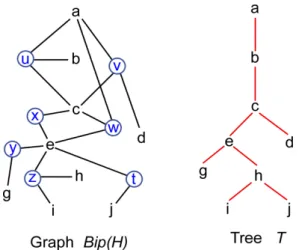
set g(u). The width of (T, f) and the tree-width twd(H) of H together with the notions of normal, clean and quasi-normal tree-decompositions are as for K(H). Figure 3 shows the graph G = Bip(H) associated with a 3-hypergraph H with hyperedges t, u, v, w, x, y, z and the tree T of a tree-decomposition (T, f ) of H of width 2; the function f is defined in the following table (s ∈ NT). In
the figure, hyperedges are circled, and the edges of Bip(H) are undirected. s f(s) s f (s) a a g g, e b b, a h h, e c c, b, a i i, h, e d d, c, a j j, e e e, c, a
Lemma 21: (1) For every hypergraph H, twd(Bip(H)) ≤ twd(H) + 1 and twd(H) is unbounded in terms of twd(Bip(H)).
(2) If H is a q-hypergraph, then twd(H) ≤ q(twd(Bip(H)) + 1) − 1.
Proof sketch : (1) Let (T, f ) be a tree-decomposition of H. For each hyperedge e, there is a node u of T such that all vertices of e are in f (u) and we add to T a new son u′ of u with associated set {e} ∪ f(u). We get a
tree-decomposition of Bip(H) of width twd(Bip(H)) + 1.
(2) Let (T, f ) be a tree-decomposition of Bip(H) of width k such that H is a q-hypergraph. We define f′(u) :=
f (u) ∪ {x ∈ VH| incH(x, e) for some e ∈ f(u) ∩ EH} − (f (u) ∩ EH).
Then (T, f′) is a tree-decomposition of H and |f′(u)| ≤ q |f(u)| ≤ q(k + 1)
Figure 3: Bip(H) and the tree T of a tree-decomposition of H.
Remarks : (1) We do not have twd(Bip(H)) ≤ twd(H) in general: let H be the hypergraph with 3 vertices and 3 hyperedges containing all these vertices. Then, twd(H) = 2 but twd(Bip(H)) = 3 (because Bip(H) contains K4 as a
minor).
(2) One cannot bound twd(H) in terms of twd(Bip(H)) alone : if H has one hyperedge with n + 1 vertices, we have twd(Bip(H)) = 1 and twd(H) = n.
This lemma shows that for fixed q, the tree-width of a q-hypergraph and that of its associated bipartite graph are linearly related. Theorem 19 shows that cwd(Bip(H)) = O(twd(Bip(H))q) for a q-hypergraph. We have cwd(Bip(H)) =
O(twd(H)q) by this fact and Lemma 21 but we can do better.
Theorem 22: Let q ≥ 2. For every q-hypergraph H, we have: cwd(Bip(H)) ≤ γ(twd(H) + 1, q − 1) + 1 = O(twd(H)q−1).
Proof: Let (T, fT) be a normal tree-decomposition10 of H, i.e. of K(H),
of width k = twd(H). The vertices of a hyperedge e are in fT(u) for some node
u of T , hence are linearly ordered by ≤T because (T, fT) is normal; we let e be
the smallest one.
We extend T into a tree U with set of nodes NT ∪ EH as follows. For each
u ∈ VH, we let e1, ..., em be the hyperedges e such that e = u; we replace the
edge u − pT(u) of T by the path u − e1− ... − em− pT(u); if m = 0 we do
nothing; if u is the root, we put the path e1− ... − emabove u with emas new
root (these hyperedges have u as unique vertex). The vertices of a hyperedge e are e that is below it (in U ), and, at most q − 1 vertices that are above.
1 0The mapping f
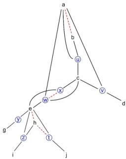
Figure 4: Tree U for Bip(H) of Figure 2.
Figure 4 shows Bip(H) and the tree U for H and T of Figure 3. The edges of U not in Bip(H) are shown with dotted lines. The nodes for hyperedges w and x are inserted between e and c. We could have inserted x below w.
It is clear that U is a normal tree for Bip(H). We obtain a normal tree-decomposition (U, fU) of Bip(H). (It is not the tree-decomposition constructed
in the proof of Lemma 21(1); its width is not bounded in terms of k: just consider several parallel edges between two vertices.) In order to use Theorem 11, we bound the cardinalities of the sets Ω(U<(w), fU(w)).
If w ∈ VH, then Ω(U<(w), fU(w)) consists of the following sets:
first, the sets NBip(H)(u) ∩ fU(w) for u ∈ VH, u <U w; these sets are
empty, because the neighbours in Bip(H) of such u are hyperedges e such that e <T u or e = u but, in both cases, e <T w, hence
e /∈ fU(w);
second, the sets NBip(H)(e) ∩ fU(w) for e ∈ EH, e <U w; these sets
are subsets of fT(w) of cardinality at most q−1, because they are the
sets of ends v ≥T w of the edges of K(H) whose other end is e <U e;
(in the example of Figure 4, for w := c, the sets in Ω(U<(w), fU(w))
are ∅, {c} and {a, c}).
Hence, |Ω(U<(w), fU(w))| ≤ γ(k + 1, q − 1).
first, the sets NBip(H)(u) ∩ fU(e) for u ∈ VH, u <U e: if u = e,
then NBip(H)(u) ∩ fU(e) = N (e) := {e1 ∈ EH | e ≤U e1, e1 = e},
otherwise, u <T e, and the neighbours of u are hyperedges e1 <U
e <U e, hence, NBip(H)(u) ∩ fU(e) = ∅; (in the example of Figure 4,
we have N(wO) = {wO, xO} where wO denotes the "circled w" and
similarly for xO; we have N (xO) = {xO});
second, the sets NBip(H)(e1) ∩ fU(e) for e1 ∈ EH, e1 <U e: these
sets are subsets of f∗
T(e) of cardinality at most q − 1, because they
are the sets of ends v ≥ e > e of the edges of K(H) whose other end is below e, hence below e or equal to it; (in the example of Figure 4, we have NBip(H)(wO) ∩ fU(xO) = {a, c}).
Hence, |Ω(U<(w), fU(w))| ≤ 1 + γ(k, q − 1) ≤ γ(k + 1, q − 1). The claimed
result11 follows then from Theorem 11.
5.2
Incidence graphs
Let G be undirected, possibly with loops and parallel edges. Its incidence graph Inc(G) is the bipartite graph (VG ∪ EG, incG) such that incG := {(v, e) ∈
VG×EG| v is a vertex of e}. A loop has degree one in Inc(G). If G is considered
as a 2-hypergraph, then Inc(G) = Bip(G). If G is directed, then Inc(G) is defined as (VG∪ EG, incG) with incG := {(v, e) ∈ VG× EG | e : v →G w for
some vertex w} ∪ {(e, v) ∈ EG× VG | e : w →Gv for some vertex w}.
Tree-width and clique-width for G and Inc(G) are related as follows: twd(G) ≤ twd(Inc(G)) ≤ twd(G) + 1 and12
twd(Inc(G)) ≤ 6cwd(Inc(G)) − 1 by Theorem 10(2).
The following corollary of Theorem 22 is proved in [4] in a different way.
Corollary 23: We have cwd(Inc(G)) ≤ twd(G) + 3 if G is undirected and cwd(Inc(G)) ≤ 2twd(G) + 4 if it is directed.
Proof: If G is undirected, Theorem 22 yields that the clique-width of Inc(G) = Bip(G) is bounded by γ(twd(G) + 1, 1) + 1 = twd(G) + 3.
If G is directed, we construct U as in the proof of Theorem 22. In that case, every edge e of G that is not a loop links a vertex e below it in U and one above it. If it is a loop, then e → e and e → e. We use the notation of the proof of Theorem 11 for directed graphs. The sets Ω(U<(w), fU(w)) consist of the pairs
(NInc(G)+ (u) ∩ fU(w), NInc(G)− (u) ∩ fU(w)) for u <U w.
1 1A similar result in [4] states that cwd(S(H)) = O(twd(H)q−1) if H is a q-hypergraph and
S(H) is Bip(H) augmented with undirected edges between any two vertices of H.
1 2If G is simple and undirected, then twd(G) = twd(Inc(G)). If G consists of two opposite
If w ∈ VG, Ω(U<(w), fU(w)) consists of (∅, ∅) and pairs (v, ∅) or (∅, v) for
some v ∈ fU(w). Hence, |Ω(U<(w), fU(w))| ≤ 1 + 2(k + 1).
If w = e ∈ EG, then Ω(U<(w), fU(w)) consists of (∅, ∅), the pair (NInc(G)+ (e)∩
fU(e), NInc(G)− (e) ∩ fU(e)) and pairs (v, ∅) or (∅, v) for some v ∈ fT(e) − {e}.
Hence, |Ω(U<(w), fU(w))| ≤ 1 + 1 + 2k < 2k + 3. We obtain the bound 2k + 4
by Theorem 11.
Remark 24 : The empty set (or the pair (∅, ∅)) is used in the construction of a term that denotes Inc(G) as a label for its vertices in VGas well as in EG. In
view of application to the model-checking of MSO2properties (see Section 6 and
[7, 8]), it is useful to distinguish labels for vertices in VG from those for vertices
in EG. In that case, we duplicate these "empty" labels (and no others). So, we
can construct Inc(G) with two labels for the vertices of G and twd(G)+ 2 labels for its edges, i.e., the vertices in EG⊆ VInc(G). If G is directed these figures are
respectively 2 and 2twd(G) + 3.
6
Algorithmic applications
We discuss some applications of our constructions to the verification of monadic second-order expressible graph properties (MSO properties in short) by means of automata that process clique-width terms denoting the input graphs. This method is implemented in the running system AUTOGRAPH13. This section being informal, we will use examples and we refer the reader to [12, 9] for definitions.
6.1
Model-checking with fly-automata
We give the example of a monadic second-order (MSO) sentence14 expressing
that a graph G, defined as the relational structure VG, edgG , is 3-colorable.
This sentence is ∃X, Y.Col(X, Y ) where Col(X, Y ) is the formula X ∩ Y = ∅ ∧ ∀u, v.{edg(u, v) =⇒
[¬(u ∈ X ∧ v ∈ X) ∧ ¬(u ∈ Y ∧ v ∈ Y )∧ ¬(u /∈ X ∪ Y ∧ v /∈ X ∪ Y )]},
expressing that X, Y and VG−(X ∪Y ) are the three color classes of a proper
3-coloring of the considered graph G.
An MSO sentence intended to express a graph property can only use quan-tifications over vertices and sets of vertices. More powerful are the MSO2
sen-tences, that can also use quantifications over edges and sets of edges. We recall the following "algorithmic meta-theorem" [12, 14, 16, 17].
1 3AUTOGRAPH can even compute values associated with graphs [11], for an example, the
number of 3-colorings. It is written in Common Lisp by I. Durand. See http://dept-info.labri.u-bordeaux.fr/~idurand/autograph.
Theorem 25 : (a) For every integer k and every MSO sentence ϕ, there exists a linear-time algorithm that checks the validity of ϕ in any graph given by a term in T (F[k]), whence of clique-width at most k. The computation time
is linear in the size of the term.
(b) For every integer k and every MSO2 sentence ϕ, there exists a
linear-time algorithm that checks the validity of ϕ in any graph given by a tree-decomposition of width k, whence of tree-width at most k. The computation time is linear in the size of the tree-decomposition.
Assertion (b)15 is actually a consequence of (a) because :
(1) an MSO2property of a graph G is nothing but an MSO property
of its incidence graph Inc(G),
(2) if G has tree-width k, then Inc(G) has clique-width at most f (k) for some fixed linear function f (cf. Corollary 23), and
(3) a tree-decomposition of G of width k can be converted in linear time (for fixed k) into a clique-width term of width at most f (k) that defines Inc(G).
Point (1) is just a matter of definitions. Point (2) and the linear-time trans-formation of (3) make practically usable this reduction of (b) to (a). This fact is developped in [7, 8]. MSO2 sentences are more expressive than MSO ones,
but bounded tree-width is necessary for having FPT algorithms to check the corresponding properties in this way, via incidence graphs.
Some linear-time algorithms intending to implement (a) use finite automata that take as input terms t in T (F[k]) and answer whether the graph G(t) satisfies
the considered property. However, these automata are much too large to imple-mentable in the classical way by means of transition tables. To the opposite, fly-automata (FA in short) compute the transitions that are needed during the run on a given term and thus overcome the size obstacle.
We review FA informally. Let C be a countably infinite set of labels. A deter-ministic fly-automata A over FChas a possibly infinite set of states QA⊆ (C ⊎
B)∗where B is a finite set of auxiliary symbols, typically T rue, 0, 1, (, ), {, },”, ” etc. Its transitions are of the forms a →A p, f [q] →A p and ⊕[q, q′] →A p,
where a ∈ C, f ∈ FC is unary, q, q′, p ∈ QA and p is defined in a unique way
by an algorithm (that is part of the definition of A) from a, or from f and q, or from q and q′. The (possibly infinite) set Acc
A ⊆ QA of accepting states
is decided by an algorithm. It follows that, on each term t, the automaton A has a unique (bottom-up) run. This run is computable and so is qA(t), the
1 5By a result of Bodlaender (see [3, 16, 17]), a tree-decomposition of G of width k can be
computed in linear time if there exists one. Hence the variant of (b) where a tree-decomposition is not given but must be computed also holds, but this variant is not a consequence of (a). Furthermore, the linear time decomposition algorithm is not practically implementable.
(unique) state reached at position ε (the root of the syntactic tree of t). Hence, the membership of t in L(A), the langage accepted by A, is decidable.
The time computation of a deterministic FA A on a term t is Σ{τA(u) |
u ∈ P os(t)} where τA(u) is the time taken to compute the state p reached at
position u by the run of A, plus the time taken to check whether qA(t) ∈ AccA.
For model-checking, we are interested in cases where t ∈ L(A) if and only if G(t) satisfies the property to check. Note that the same automaton, hence, the same algorithm, works for graphs of any clique-width as C is infinite.
Example 26 : A deterministic fly-automaton A that checks 3-colorability. Let Γ := {1, 2, 3} be the set of colors. Let G be a C-labelled graph. For each mapping γ : VG → Γ, we define γ := {(a, i) ∈ C × Γ | γ(x) = i for some
a-labelled vertex x}.
We define ξ(G) as the finite set of finite sets γ such that γ is a proper 3-coloring of G (no two adjacent vertices have the same color). For t ∈ T (FC), we
define ξ(t) := ξ(G(t)). Clearly, ξ(t) can be written as a word over C ⊎ Γ ⊎ A where A is the alphabet consisting of (,),{,} and ",". The function ξ satisfies the following inductive property :
ξ(a) = {{(a, 1)}, {(a, 2)}, {(a, 3)}} for a ∈ C, ξ(adda,b(t)) = {α ∈ ξ(t) | there is no i = 1, 2, 3
such that (a, i) and (b, i) belong to α}, ξ(relabh(t)) = h(ξ(t)) where h replaces in the word ξ(t)
each label a ∈ C by h(a), ξ(t1⊕ t2) = {α ∪ β | α ∈ ξ(t1), β ∈ ξ(t2)}.
These properties give the transitions of the desired FA A whose set of states is P(P(C × Γ)), identified to a language over C ⊎ Γ ⊎ A, and such that qA= ξ.
The transitions are:
a→A{{(a, 1)}, {(a, 2)}, {(a, 3)}},
adda,b[q] →A{α ∈ q | there is no i = 1, 2, 3
such that (a, i) and (b, i) belong to α}, relabh[q] →Ah(q),
⊕[q, q′] →
A{α ∪ β | α ∈ q, β ∈ q′}.
All states are accepting except the empty set. The set of all states that can occur in a run over a term in T (F[k]) (assuming [k] ⊆ C) is finite but of
cardinality 223k
. Hence, it cannot be listed in a table for useful values of k.
We go back to the general case. We fix C. If ϕ is an MSO sentence, we denote by L(ϕ) the set of terms t ∈ T (FC) such that G(t) |= ϕ. The proof of