HAL Id: hal-01350517
https://hal.archives-ouvertes.fr/hal-01350517
Submitted on 7 Sep 2016
HAL is a multi-disciplinary open access
archive for the deposit and dissemination of
sci-entific research documents, whether they are
pub-lished or not. The documents may come from
L’archive ouverte pluridisciplinaire HAL, est
destinée au dépôt et à la diffusion de documents
scientifiques de niveau recherche, publiés ou non,
émanant des établissements d’enseignement et de
Structural simplification of chemical reaction networks
in partial steady states
Guillaume Madelaine, Cédric Lhoussaine, Joachim Niehren, Elisa Tonello
To cite this version:
Guillaume Madelaine, Cédric Lhoussaine, Joachim Niehren, Elisa Tonello. Structural simplification
of chemical reaction networks in partial steady states. BioSystems, Elsevier, 2016, Special Issue of
CMSB’2015, 149, pp.34–49. �10.1016/j.biosystems.2016.08.003�. �hal-01350517�
Structural simplification of chemical reaction networks in partial steady states
IGuillaume Madelainea,b,⇤, Cédric Lhoussainea,b, Joachim Niehrena,c, Elisa Tonellod
aCRIStAL, UMR 9189, 59650 Villeneuve d’Ascq, France bUniversity of Lille, France
cINRIA Lille, France
dUniversity of Nottingham, United Kingdom
Abstract
We study the structural simplification of chemical reaction networks with partial steady state semantics assuming that the concentrations of some but not all species are constant. We present a simplification rule that can eliminate interme-diate species that are in partial steady state, while preserving the dynamics of all other species. Our simplification rule can be applied to general reaction networks with some but few restrictions on the possible kinetic laws. We can also simplify reaction networks subject to conservation laws. We prove that our simplification rule is correct when applied to a module of a reaction network, as long as the partial steady state is assumed with respect to the complete network. Michaelis-Menten’s simplification rule for enzymatic reactions falls out as a special case. We have implemented an algorithm that applies our simplification rule repeatedly and applied it to reaction networks from systems biology. Keywords: bioinformatics; systems biology; reaction network; contextual equivalence.
1. Introduction
Reaction networks [1] are systems of chemical
reac-tions, which are widely used in systems biology [2] in
order to model and analyze the dynamics of molecular
biological systems [3,4,5]. Reaction networks have a
formal semantics that describes the evolution of chemical solutions over time (without fixing the initial solution). This semantics lays the foundation for formal analysis of biological systems. In the present paper, we focus on the deterministic semantics which, in the thermodynamic
limit [6], describes the average concentrations of species
in chemical solutions, rather than considering the stochas-tic semanstochas-tics which models their probability distributions. Formal analysis methods for biological systems are based on their reaction networks. If all kinetic
parame-IThis work has been funded by the French National Research
Agency research grant Iceberg ANR-IABI-3096.
⇤Corresponding author:guillaume.madelaine@ed.univ-lille1.fr
ters are known, reaction networks can be used to
simu-late biological systems [7]. Otherwise, the missing
pa-rameters can be estimated so that they fit with
experi-mental data [8]. Reaction networks can also be used to
verify properties of biological systems [9], to control
bi-ological systems in real time [10], or to predict network
changes such as gene knockouts leading to desired
behav-ior [11,12,13]. The analysis techniques to solve these
tasks may be either numeric or symbolic. Numeric tech-niques are usually based on the ordinary di↵erential equa-tions (Odes) for the deterministic semantics only, while assuming the knowledge of all parameters. Symbolic analysis methods, in contrast, may be based on the struc-ture of a reaction network and not only the Odes. Struc-tural methods are sometimes advantageous as argued in
[14] for instance.
Given that biological systems are highly complex, their models by reaction networks may become huge (see
e.g. [15]). Furthermore, a large number of kinetic
formal analysis techniques. Possible workarounds are to analyze only smaller modules of reaction networks, or to simplify bigger reaction networks in order to reduce their size and the number of their unknown parameters. There-fore, various simplification methods for reaction networks
were developed (see [16] for an overview), often
moti-vated by Michaelis-Menten’s seminal reduction of
enzy-matic reactions [17].
Structural simplification methods that rewrite reaction networks rather than Odes are particularly relevant for bi-ological modeling. Indeed, biologists are spending much e↵ort in designing reaction networks in practice, as for instance on the development of the metabolic and
regula-tion networks for B. Subtilis in the Subtil Wiki [15]. Even
though many of the reactions used there are motivated by structural simplification of larger reaction networks with more details, no such formal justification is given.
A purely structural simplification method for reaction
networks without kinetic rates was developed in [18]. It
consists of a set of rewrite rules that remove intermediate species in reaction networks. For instance, we can sim-plify the network with the following two reactions on the left into the single reaction on the right, when considering B as an intermediate species:
A1+ . . . +AnA B
B A C1+ . . . +Cm
)
V A1+. . .+AnA C1+. . .+Cm (1)
These two networks perform the same transformations on chemical solutions that do not contain intermediate B molecules, if one ignores intermediate results. Indeed, this simplification rule is correct with respect to the
at-tractor equivalence (also proposed in [18]). There, a
reac-tion network is considered as non-deterministic program (operating on multisets), so that notions of observational
program semantics from compiler construction [19] can
be applied. A main weakness of this approach is that it can neither deal with kinetic rates nor with deterministic Ode semantics. Furthermore, some other rules for inter-mediate elimination, that one might want to have, turn out to be incorrect, as for instance:
A A B
A0+B A C
)
V A + A0A C (2)
To see the di↵erent input-output behavior, consider the
multiset nA + 0A0+0B. With the reaction network on
the left, this chemical solution can be transformed to
0A + 0A0+nB, while with the reaction on the right no
transformation is possible.
An approach for the structural simplification of reaction networks with kinetic rates subject to Ode semantics was
presented by Radulescu [20,16]. The basic idea is also
to remove intermediate species in reaction networks, but now assuming that the intermediate species are in quasi steady state. In a first phase, the graph structure of the reaction network is simplified. But rather than eliminat-ing the intermediate species step by step, elementary flux
modes [21] are computed in order to remove all
interme-diates simultaneously. The kinetic rates are then assigned to the simplified network, under the condition that the in-termediates were in quasi steady state. Interestingly, the
simplification rule in (2), which is wrong with respect to
the nondeterministic attractor equivalence, becomes cor-rect for the deterministic Ode semantics, when assum-ing that the concentrations of the intermediate species are steady. The point is that the concentration of B is not
steady in the chemical solution nA + 0A0+0B on which
the reaction network on the left could act but not the one on the right. Indeed a key idea of Radulescu’s approach is to resolve the steady state equations for an intermediate
species B after its concentration variable xB. Since this is
not always possible in an exact manner, an approximate method is proposed. The main weakness of the approach is that its correctness is not formally stated. The two main obstacles on the way to a correctness statement are the use of approximations, and the fact that kinetic rates are assigned only at the end to the reduced network.
The objective of the present article is to overcome the shortcomings of the two previous approaches. We search for a rewrite rule that can eliminate intermediate species in reaction networks with kinetic rates while exactly pre-serving the Ode semantics. Furthermore, our rewrite rule should remain correct when applied to a module of a re-action network, and should remain applicable when the parameters of the kinetics laws are unknown. For this, we are ready to assume that the concentration of inter-mediate species are steady, i.e. that the concentration of
the intermediate B satisfies xB=c for some positive
con-stant function c. Such partial steady state assumptions are more flexible than general steady state assumptions in that the concentrations of some species may still change over time. In contrast to quasi steady state assumptions no
ap-proximation is made.
The present article extends a conference paper at
CMSB’2015 [22]. The contributions are as follows. We
first present a rewrite rule for the structural simplification of reaction with kinetic rates, which removes one interme-diate species at a time. In order to avoid approximations, we assume that all kinetic rates of the network are either linear in the concentration of the intermediate species, or else constructed in a uniform manner by applying some invertible function. More precisely, for any intermediate species B, there must be an invertible function f , common to all reactions consuming B, and such that their kinetic
laws are some product of the form f (xB)e, where e is an
expression not containing xB and possibly varying with
the reactions. We second prove that our rewrite rule does preserve the Ode semantics of the reaction network, even if the network is plugged into any possible context. Com-pared to the conference version we permit networks with conservation laws. For instance, such an expression may
impose that xA+xB=c for some positive constant
func-tion c, i.e., that the sum of the concentrafunc-tions of A and B is steady. Beside of being more general, the addition of conservation laws also simplifies the presentation of the rewrite rule and of the correctness proof.
An interesting question is whether repeated elimination of intermediates with our rewrite rule does always pro-duce the same set of results as Radulescu’s simplification method. As we worked out in detail in a follow up paper
[23], this is not the case. The point is that by the
compu-tation of elementary modes one does also eliminate "de-pendent reactions" – that is linear combinations of others – that are generated by the elimination of intermediates.
rrrr Similar results as here were developed in parallel
and independently by Saez et al. [24]. They also propose
an exact method for the elimination of linear intermediate species in partial steady state, and prove that it preserves the deterministic Ode semantics. Their procedure elimi-nates several intermediate species in one big step. Clearly, the objective of simultaneous elimination subsumes that of single intermediate elimination, as in the present paper. Compared to Radulescu’s method, which also supports si-multaneous elimination, it is based on the computation of the spanning trees of the graph of intermediates, instead of using elementary modes. The kinetic functions are sup-posed to be linear in the intermediates, which is one of the two possible restrictions considered in the present paper.
This restriction combined with the spanning tree method enables them to prove a formal correctness result for their simultaneous intermediate elimination. A major di↵er-ence of Saez reduction method to the present article and Radulescu’s approach is that it always produces a unique reduced network as a result. We believe that the same net-work can always be obtained by repeated elimination of intermediate species and dependent reactions, but many di↵erent results are possible thereby too. We refer to the
confluence study in [23] for further discussions of this
topic.
Outline. In Section 2, we illustrate our simplification
method with two examples. First we revisit Michaelis-Menten’s reduction rule, and then we illustrate how one can simplify a small gene expression network with inhibi-tion. We recall the formal definitions of reaction networks
in Section3, and of conservation laws in Section4. In
Section5, we contribute a contextual equivalence relation
for reaction networks, and in Section6a set of
simplifica-tion rules, that we prove correct with respect to this
equiv-alence relation. In Section7, we illustrate, with biological
examples, how much reaction networks can be simplified in practice. We then discuss further related work in
Sec-tion8, and the relevance of our results in Section9. We
conclude and discuss future work in Section10.
2. Motivating Examples
We first revisit Michaelis-Menten simplification rule for an enzymatic reaction network, and illustrate how the notions of modules and contexts of reaction networks in-tervene there. We then illustrate how the same ideas can be lifted to more general reaction networks by looking at the example of an inhibited gene expression.
Let R+ be the set of nonnegative real numbers t 0.
Kinetic expressions will denote positive real functions
that map time points in R+ to concentrations in R+. We
denote by C the set of all positive constant functions
C = { f : R+ ! R+| f (0) = f (t) 0 for all t 2 R+}.
2.1. Michaelis-Menten revisited
The Michaelis-Menten simplification rule applies to the following enzymatic reaction network with three
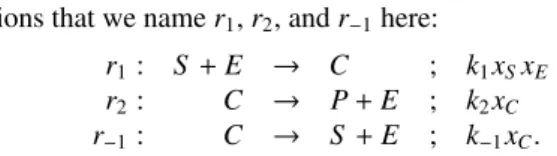
reac-tions that we name r1, r2, and r 1here:
r1: S + E ! C ; k1xSxE
r2: C ! P + E ; k2xC
r 1: C ! S + E ; k 1xC.
Substrate S and enzyme E must first build a complex C
via r1, before C can produce product P and free enzyme E
by r2. Alternatively, complex C can also be redecomposed
into S and E by r 1. All three reactions must satisfy the
mass action law with di↵erent rate constants k1, k2, and
k 1respectively as as specified by the kinetic expressions.
The variables xS, xE, and xCin the kinetic expressions
de-note some positive real functions, which specify the evo-lution of the concentrations of the respective species over time.
See Figure1for an illustration of this reaction network
as a Petri-net. The dotted arrows on S and P mean that these species can be produced or consumed by admissible contexts, while the other species C and E cannot. The Odes system of this network can be derived as usual and
are presented in Fig.2.
The idea of Michaelis-Menten simplification rule is to eliminate the intermediate C from the system, under the assumption that the concentration of C is steady, or in other words, when considering only those solutions of the
Odes of the reaction network in which xC =cCfor some
positive constant function cC 2 C. Clearly, the value of
the constant function cCmust then be equal to xC(0), i.e.,
to the initial concentration of C at time t = 0. For other initial concentrations, where this assumption is not satis-fied, there is still hope for approximate correctness with some kind of quasi steady state assumptions, but this kind of arguments is out of the scope of the present paper. Lemma 1. When considering this reaction network in isolation and not as a module of a larger network, any solution of its Odes where C is in partial steady state must satisfy:
• dxdtC =0, and
• xS, xE, and xPare constant, and
• if xE, 0 then xS =0.
Proof. This can be seen as follows. If C is in partial
steady state then xC =cCfor some positive constant
func-tion cC 2 C. HencedxdtC =0. By observing that the two
dxS dt = k 1xC k1xSxE dxE dt = (k2+k 1)xC k1xSxE dxC dt = (k2+k 1)xC+k1xSxE dxP dt = k2xC
Figure 2: Odes system for Michaelis-Menten module with 3 enzymatic reactions without any context.
Odes for derivations of E and C are equal up to the sign,
it follows that dxdtE = dxC
dt =0 and so that xE =cEfor
some positive constant function cE 2 C. From the Ode for
the derivation of C we obtain the linear equation:
(k2+k 1)cC=k1xScE (3)
If cE =0 then the proposition follows straightforwardly.
Otherwise, cE , 0 so that xS = (k2+kk1cE1)cC is constant. The
di↵erential equation for S can now be reduced to follow-ing linear equation:
k-1cC=k1xScE (4)
In combination, equations (3) and (4) yield cC =0. From
this, equation (4) again implies xS = 0 since cE , 0.
Furthermore, cC = 0 implies dxdtP = 0 so that xP is
con-stant.
The situation becomes more interesting when the net-work is considered as a module of a larger netnet-work. For instance, we can consider the admissible context that adds one reaction for an inflow of substrate S with constant
speed kiand another reaction that models an outflow of
product P with linear speed koxP:
substrate inflow: ; ! S ; ki
product outflow: P ! ; ; koxP.
Any partial steady state for C of the extended network, unifying the module with the three enzymatic reactions and the context with the two reactions modeling inflows
S E C P r1 k1xSxE r 1 k 1xC r2 k2xC .9cC2 C. xC=cC S r P k2cC .9cC2 C. cC = kk1xSxE 2+k 1
Figure 1: Basic step of Michaelis-Mentens simplification rule under the assumption that C is in partial steady state.
and outflows, must verify xC =cCfor some positive
con-stant function cC2 C satisfying:
cC= kk1xSxE
2+k 1. (5)
Therefore, the Ode of the extended network can be sim-plified to:
dxP
dt =k2cC koxP
while keeping (5) as a conservation law. In analogy, but
independently of any context, we can simplify the mod-ule with the three enzymatic reactions into the following reaction r:
r : S ! P ; k2cC
As we will see, this simplification of the module is correct for all its admissible contexts, when assuming that C is in partial steady state.
So far, the kinetics of the reduced network still look quite di↵erent from usual Michaelis-Menten kinetics. But
if we assume in addition the conservation law xE+xC =
ctotal
E for some constant function ctotalE 2 C designing the
total enzyme concentration, then it follows by elementary calculations, that: cC=ctotalE xS xS +k1+k2 k1 .
Hence, we do indeed obtain the classical Michaelis-Menten law by our simplification procedure.
It should be noticed that our assumption that cCis
con-stant is equivalent to that xS
xS+k 1+k2k1 is constant, and thus
to the assumption that xS is constant. The latter might
look problematic with respect to the usual of
Michaelis-Menten law. Since if xS is not constant for some initial
conditions, then this initial concentration of S may be at best close to a value for which C will be in partial steady state. Therefore, the dynamics of the simplified network may be at best an approximation of the original dynam-ics. Further arguments would be in order to establish such an approximation, but these are out of the scope of the present article.
2.2. Inhibited Gene Expression
In order to illustrate the main ideas of our proposal, we next consider the reaction network Gene of inhibited gene
expression in Fig.3.
This reaction network has four species: gene G, in-hibitor Inh, messenger RNA mRNA, and protein P. It also
has four reactions: reaction r1 describes a transcription,
the production of mRNA in presence of gene G. This re-action has also an inhibitor, Inh, that slows down the
reac-tion. G and Inh are modifiers in r1, indicated by a dashed
arrow in the figure, meaning that they influence the speed rate of a reaction, but that the reaction does not modify
their amounts. Reaction r2is the translation of mRNA into
protein P, while reaction r3(resp. r4) describes the
degra-dation of mRNA (resp. P). Except for reaction r1with the
inhibitor, all other reactions have mass-action kinetics. Before attempting to simplify the network, we need to specify how the context may interact with it: this is
in-dicated by pending dotted arrows in Fig.3. We consider
here that G and mRNA are internal species, that is, which can not be modified by the context. Then, the context can
G Inh mRNA P r1 k1xG k0+xInh r2 k2xmRNA r3 k 1xmRNA r4 k 2xP .9cmRNA,cG2 C. xmRNA=cmRNA^ xG=cG Inh mRNA P r1 k1cG k0+xInh r2 k2xmRNA r3 k 1xmRNA r4 k 2xP .9cmRNA,cG2 C. xmRNA=cmRNA Inh P r123 k2cmRNA r4 k 2xP .9cmRNA,cG 2 C. cmRNA= k k1cG 1(k0+xInh)
Figure 3: Graph of the reaction network Gene on the left, and its two simplifications. Molecular species are represented by circles, and reactions by squares. In the kinetic expressions near the reactions, the kiare parameters while xAis a variable representing the concentration of a species A.
The variable cGdenotes the initial concentration of G which is assumed to remain constant, by imposing the conservation law xG=cGfor some
positive constant function cG2 C. A dashed arrow means that the molecule acts as a modifier in the reaction, while a dot arrow means that the
molecule can be modified by the context.
be any set of reactions that does not involve G and mRNA. It can for instance transform P into another protein, or produce something else in presence of Inh, etc.
In this network, we are especially interested in the dy-namics of protein P. Therefore, we will say that P is an observable species, that we should not remove. On the other hand, we will assume that the intermediate mRNA is
at steady state, i.e. that xmRNA =cmRNAfor some constant
function cmRNA 2 C. Hence, we want to eliminate mRNA
in particular.
In order to simplify the network, we first notice that gene G is not modified by any reaction, and that it can not be modified by any context, since it is assumed internal. Therefore its concentration is constant over time, as
de-scribed in the conservation law xG = cG. Hence, we can
remove G from the network by replacing xG by cG, and
removing the conservation law. This results in the
simpli-fied network in the middle of Fig.3.
Now, consider the intermediate mRNA. It is an internal species, satisfying the following Ode independently of the context:
dxmRNA
dt =
k1cG
k0+xInh k 1xmRNA.
Since we assumed that mRNA is at steady state with
xmRNA = cmRNA, we have dxmRNAdt = 0, so that we can
deduce the conservation law:
cmRNA= k k1cG
1(k0+xInh).
Therefore we can remove mRNA from the network, and
replace the variable xmRNA by a constant cmRNA in the
ki-netics of reaction r2, while adding the above conservation
law. We obtain the simplified network on the right of Fig.
3. The three reactions r1, r2 and r3that produce or
con-sume the intermediate mRNA or use it as a modifier are
merged into the new reaction r123.
Note that sometimes, the steady state assumptions en-tail some other implicit conditions. For the Michaelis-Menten simplification rule, the simplification implied that
xS was constant, as discussed above. In this example, the
fact that mRNA is at steady state entails that the concentra-tion of the inhibitor Inh needs to be constant too. This im-plicit condition is still present in the simplified network,
with the conservation law cmRNA= k k1cG
1(k0+xInh).
to be constant to perform the simplification. However, we do not impose a total steady state. For instance, the con-centration of the protein of interest P could still change over time. Its dynamics will be the same in both the ini-tial and simplified network.
As we will see in this paper, the simplification rules used above preserve the deterministic semantics of reac-tion networks, in every context. Hence the simplified net-work is contextually equivalent to the first one. Note that we can not simplify the network anymore, since P is an observable species, and that both Inh and P can be modi-fied by the context.
3. Syntax and semantics of reaction networks
Let Spec be a finite set of molecular species ranged over by A. For instance, we used Spec = {Inh, mRNA, G, P} for the gene expression network.
We define a (chemical) solution s 2 Sol : Spec ! N0
as a multiset of molecular species, i.e. a function from molecular species to natural numbers, with a finite
sup-port. Given natural numbers n1, . . . ,nk, we denote by
n1A1+ . . . +nkAkthe solution that contains nimolecules
of species Aifor all 1 i k and 0 molecules of all other
species. ni is called the stoichiometric coefficient of Ai
in the solution. We define the intersection and di↵erence
of two solutions by (s1\ s2)(A) = min(s1(A), s2(A)) and
(s1 s2)(A) = s1(A) s2(A).
A reaction r = (s1A s2; e) 2 Reactions is a pair
com-posed of two solutions s1and s2, and a kinetic expression
e. The reaction transforms the solution s1, of so called
reactants, into the solution s2, of so called products. We
denote by scr(A) = s2(A) s1(A) 2 Z the stoichiometric
coefficient of A in the reaction r, and by kin(r) = e the kinetic expression of r. We consider a countable set of variables Vars that contains, for any A 2 Spec, a variable
xAfor a concentration, and a variable cA, that we will use
later to define the steady state assumption. We also have a
set of kinetic parameters Param = {k0,k1, . . .}. Kinetic
ex-pressions are terms describing kinetic functions, that have the following abstract syntax:
e, f ::= x | k | | e + f | e f | e ⇤ f | e/ f | e
where x 2 Vars, k 2 Param and 2 R. As usual, we
also simply denote e f for e ⇤ f , and use parenthesis (e)
whenever the priority of the operators might not be clear. We denote by Vars(e) the set of variables of e.
A normalized reaction is a reaction in which the reactants and the products do not have shared molecules,
i.e. s1\ s2 = ;. Given a reaction r = (s1A s2; e) and
s = s1 \ s2, we denote the corresponding normalized
reaction by er = (s1 s A s2 s; e). Trivially, for any
species A, we have scr(A) = sc˜r(A). In the following, all
reactions are assumed to be normalized.
Given a set of reactions R, we also want to merge the reactions with the same reactants and the same products.
We denote by eR the set of reactions obtained by
normal-izing and then merging the reactions in R, that is: e R = {(s1A s2; X r 2 R, er = (s1A s2; e) e) | where s1,s22 Sol}.
For now, a (normalized) reaction network R is a normal-ized set of reactions. We will later extend this definition with conservation laws.
Now, we define, as usual, the dynamics of reaction net-works in terms of ordinary di↵erential equations. Their solutions are the concentrations (depending on time) of the molecular species.
Let : Param ! R+ be the interpretation of the
pa-rameters. We assume here that is fixed to simplify the notations, but notice that our simplification is correct for any interpretation .
The (chemical) concentration of a chemical species is
a function from time to non negative numbers R+ ! R+.
Kinetic expressions are interpreted as actual kinetic
func-tions. For any V ✓ Vars, a V-assignment ↵ : V ! (R+!
R+) maps concentration variables to concentrations.
Given this assignment, the interpretation JeK↵ : R+ !
R+ of a kinetic expression e is defined by induction on
the structure of e as follows, where t 2 R+ and op 2
{+, , ⇤, /}:
JxK↵(t) = ↵(x)(t) JkK↵(t) = (k)
J K↵(t) = J eK↵= JeK↵
Je op f K↵(t) = JeK↵(t) op J f K↵(t)
Given a multiset of reactions, we only consider assign-ments ↵ such that for any kinetic expression e occurring in
this network, its interpretation JeK↵ : R+ ! R+is a
con-tinuously di↵erentiable function from time to non nega-tive real numbers, standing for the actual reaction rate.
Reactions (s1A s2; e) also have to respect the
follow-ing coherence property: if the concentration of some reac-tants is zero at some time point then the kinetic rate must
be zero too, i.e., for any species A occuring in s1, any time
point t 0, and variable assignment ↵, if JxAK↵(t) = 0,
then JeK↵(t) = 0. Note that a kinetic expression may
con-tain variables xAthat are not reactants (neither in the
prod-uct) of the reaction; such species, called modifiers, change the rate of the reaction, but the reaction does not modify their amounts.
An ordinary di↵erential equation is an equation of the form dx/dt = e, with x 2 Vars a variable and e a kinetic expression. A system of ordinary di↵erential equations is a conjunction of ordinary di↵erential equations.
For any reaction network R, we can assign it the sys-tem of ordinary di↵erential equations, denoted Ode(R), defined as follows: Ode(R) = ^ A2Spec dxA dt = X r2R scr(A)kin(r).
As expected, a reaction network and its normalized form have the same deterministic interpretation.
Lemma 2. For any R, Ode(R) = Ode(eR).
Proof. Ode(eR) = ^ A2Spec dxA dt = X (s1A s2; e)2eR scr(A)e = ^ A2Spec dxA dt = X (s1A s2; e)2eR scr(A) X r02 R, e r0=(s1A s2; e0) e0 = ^ A2Spec dxA dt = X r02R scr0(A)kin(r0) = Ode(R)
A solution of an equation dx/dt = e is a V-assignment
↵such that Jdx/dtK↵ = JeK↵, where V is the set of
vari-ables of the equation, and Jdx/dtK↵is the first derivative
of JxK↵with respect to the time t. More generally, for any
formula ', we denote by sol(') the set of V-assignments that satisfy ', with V the set of free variables of ' (in the following, some variable for non observable species will be existentially quantified).
4. Conservation law
A partial steady state assumption for a species A is a
formula of the form 9cA2 C. xA=cA, meaning that xAis
constant, and thus equivalent to the membership formula
xA 2 C. We consider consider more general formulas to
express conservation laws.
Definition. A conservation law, denoted by L, is a for-mula of the form:
9 ¯x 2 C. e1=e01^ . . . ^ em=e0m,
where ¯x = {x1, . . . ,xn} and the notation 9 ¯x 2 C. ' is a
shortcut for 9x12 C. . . . 9xn2 C. '.
For instance, the formula 9ctotal
E 2 C. xE+xC = ctotalE
in the initial Michaelis-Menten network in Figure1states
that the total concentration of the enzyme, free or bound, is constant over time.
As we saw in the preliminary examples, conservation laws need to be rewritten during the simplification. There-fore we add them to our notion of reaction networks. Definition (Reaction network with conservation law). A reaction network with conservation law N = R.L is a pair of a multiset R of chemical reactions and a conservation law L.
5. Contextual equivalence
We now introduce two other fundamental notions for our equivalence, the notion of observable species, and the notion of contexts and internal species. We then define the contextual equivalence relation of reaction networks with conservation law.
An observable species is a particularly interesting molecule, that should not be removed by the simplifica-tion, in contrast to some other molecular species that may only be relevant for some models with “low-level” details. The equivalence will then only preserve the dynamics of
these observable species. For instance, in the Gene
reac-tion network depicted in Figure3, we are especially
inter-ested in the dynamics of the protein P, that will therefore be the only observable species. We denote by O ✓ Vars the set of observable species.
We can then define a first non-contextual equivalence. Two reaction networks with conservation law are equiva-lent if they have the same deterministic deterministic dy-namics for the observable species.
Definition (Non-Contextual Equivalence). Let O be a set
of observable species, and { ˜x} = {xA | A < O} the set of
variables of unobserved species. Then the reaction
net-works N = R . L and N0 = R0.L0are non-contextually
equivalent if they have the same solutions restricted to the observable species, that is:
N ⇠O N0i↵ sol(9 ˜x. Ode(R) ^ L) = sol(9 ˜x. Ode(R0) ^ L0).
In the gene expression network, the equivalence only needs to preserve the dynamics of P, and can neglect the others.
We now extend the definition to a contextual equiva-lence. The notion of context allows us to establish equiv-alences from the equivalence of smaller and isolated sub-networks. This makes proofs of equivalences
consider-ably easier. Indeed, take two networks N1 and N2 that
di↵er only by sub-networks, that is N1 = N10[ M and
N1 = N20[ M for some N10,N20and M. With an
equiva-lence that is preserved by contexts, to prove that N1and
N2are equivalent it is sufficient to prove the equivalence
of N0
1and N20. To obtain such a desired property, one
usu-ally extends an equivalence as a congruence by closing it over all contexts. However, here, this approach would result in a too strong equivalence. In order to make signifi-cant simplifications, we will instead close our equivalence
⇠O over some contexts said to be compatible. Those are
defined from a set I ✓ Vars of molecular species called in-ternal species. A context, actually a reaction network N, is compatible with I, if 8A 2 I, A has no occurrence in N. In other words, a context compatible with I is a reaction network that does not depend and does not act on species in I. We denote by Context(I) the set of compatible con-texts with I. In the gene expression network, the internal species are I = {G, mRNA}. Then the context can interact only with the inhibitor Inh and the protein P.
Definition (Equivalence). Let O be a set of observable species and I a set of internal species, the reaction
net-works with conservation law N1 and N2 are
(contextu-ally) equivalent for O and I, denoted N1 'O,I N2, i↵
8M 2 Context(I). N1[ M ⇠O N2[ M.
Note that the sets of observable species, internal species and species at steady state are generally not the same and are independent. In the gene network, O = {P}, while I = {mRNA, G}. The species mRNA and G are also the species at steady state. In the following, we will see that we want to remove intermediate species, that are species that are non observable, internal and at steady state, like mRNA in the gene network.
6. Simplification
In this section, we present the simplification method. It is composed of a set of simplification axioms that trans-forms a reaction network into another one, smaller and equivalent.
We first present how the simplification rules work, and how to compare the size of two networks. Then we intro-duce some simple simplification rules and their proper-ties, followed by a more complex axiom, that removes an intermediate species. Finally, we show how, under some specific conditions, we can use this axiom and the conser-vation laws to remove a set of linear intermediate species. 6.1. Simplification
A simplification rule transforms a network into another one, under some conditions. The general schema for a
rule is depicted in Fig.4(left), where a network N is
sim-plified into the network M, under some particular condi-tions, and when O (resp. I) is the set of observable (resp. internal) species. Note that, after applying a simplification rule, we always directly normalize the simplified network. If we can simplify a network into another one, then we can do it in any compatible context, as depicted in the
axiom(Context)in Fig.4(right).
For any reaction network N, we denote Spec(N) the set
of species A such that either A or xAoccurs in N (i.e. in a
reaction, a kinetics or the conservation law).
We say that a network N = R . L is smaller than a
network M = R0.L0if fewer molecules occur in N than
Conditions (Name)
N '4O,I M
N02 Context(I) N'4O,I M
(Context)
N0[ N '4O,I N0[ M
Figure 4: On the left, simplification rule sketch. The network N, under the Conditions, and with the observable species O and the internal species I, can be simplified into M. On the right, the context simplification rule. If a network N can be simplified into a network M, then it is also possible in any context N0compatible with the internal species I.
• either |Spec(N)| < |Spec(M)|
• or |Spec(N)| = |Spec(M)| and |R| < |R0|.
As we will see later, the simplification rules reduce the size of networks.
We define the simplification relation'4O,Ifor the
inter-nal species I and the observable species O as the small-est equivalence relation between networks that contains
the simplifications described in Fig.4(right), Fig.5and
Fig.6. We will show that'4O,I✓'O,I, i.e. a simplified
net-work is contextually equivalent to the initial netnet-work. 6.2. Simple simplification rules
The first three simplification rules are given in Fig.5.
The first one,(Useless), deletes a reaction (; A ;; e) that
does not impact the network dynamics. The rule
(Modi-fier)removes an internal species A only used as a modifier
in the reactions (i.e. it appears in the kinetics, but not in any reactants or products). It uses a (simple) conservation law on A to compute and remove its concentration from the kinetic expression. In the simplified network, the
no-tation e[xA/eA] stands for the substitution of xA by eAin
the expression e, i.e. any occurrence of xAis replaced by
eA. This axiom is for instance used on the gene G in the
gene expression network of Section2.2.
These rules are sound for the equivalence, and reduce the size of the network.
Proposition 1. The rules (Useless) and (Modifier)
re-duce the size of the network.
Proof. Trivially, (Useless) reduces the number of
reac-tions while (Modifier) reduces the number of involved
species.
Theorem 1. The rules (Useless) and (Modifier) are
sound for the contextual equivalence, i.e. if we can sim-plify a network N into M by applying one of these rules,
then N 'O,IM.
Proof. The axiom(Useless)removes a reaction that can
not modify the concentrations of the molecules. So the Odes systems of both networks are the same, their solu-tions are equal, and the networks are equivalent.
For (Modifier), A is an internal species, and is never used as reactant or product of any reaction. Therefore its concentration is constant, and can be computed by
the conservation law xA = eA in the initial network.
Consequently, if we have a solution ↵ of the initial
net-work (in some context N0), that satisfies the
conserva-tion laws, then the Odes systems for both networks (in
the context N0) are the same, and ↵ is also a solution for
the simplified network (the additional conservation law
9cA 2 C. cA = eA is directly satisfied, since in the initial
network we have eA =xA). Reciprocally, if ↵ is solution
for the simplified network, we build the solution ↵0that
is equal to ↵, except for the species A, where ↵0
c(A) = eA.
Since eA is constant (by the conservation law) and xA is
too (since it is internal and not involved in any reaction),
↵0will still be a solution of the simplified network that
satisfies the conservation laws. Then once again the Odes
are the same, and ↵0is a solution for the initial network
too. And since ↵ and ↵0are equal modulo the intermediate
species, then the networks are contextually equivalent.
6.3. Intermediate
We now present the(Intermediate)axiom, depicted in
Fig.6, that aims at eliminating an internal, non-observable
species at steady state, by merging two-by-two the reac-tions that produce and consume it.
Let A be the intermediate (i.e. internal, non-observable and at steady state) species that we want to remove. In or-der to be able to compute systematically the kinetic rates of the simplified networks, all reactions that consume A
need to have the same kind of dependency on xA. So there
(Useless)
{(; A ;; e)} . L '4O,I ; . L
8r 2 R, scr(A) = 0 A 2 I xA< Vars(eA) (Modifier)
R . (9 ¯x 2 C. ' ^ xA=eA) '4O,I R[xA/eA] . (9 ¯x, cA2 C. '[xA/eA] ^ cA=eA)
Figure 5: Simple simplification axioms.(Useless)removes a useless reaction, while(Modifier)removes an internal species, only used as modifier and present in a simple conservation law.
N = RN.9 ¯x 2 C. ' ^ xA=cA
A 2 I A < O cA2 ¯x
split(RN, ',A, f ) = (R, R0,Rmod1,Rmod2, '1, '2)
f is a term with xA2 Vars( f )
f 1is an inverse term of f for x
Aor (Rmod2=; and '2=>) T = X (s1A s2+nA; e)2R ne T0= X (s0 1+n0A A s2; f e0)2R0 n0e0 F = T/T0 (Intermediate) N '4O,I {(n0s1+ns0 1A n0s2+ns0 2; ee0 T0) | (s1A s2+nA; e) 2 R, (s0 1+n0A A s02; f e0) 2 R0}[
{(s1A s2; e[x/F]) | (s1A s2; e[x/ f ]) 2 Rmod1}[
{(s1A s2; e[xA/f 1[xA/F]]) | (s1A s2; e) 2 Rmod2}
.9 ¯x 2 C. '1[ f /F] ^ '2[xA/f 1[xA/F]] ^ f [xA/cA] = F
Figure 6: General intermediate rule that removes the intermediate species A from reaction network N.
that the kinetic expression of any reaction with A in the
reactants is of the form f e0, with xA< Vars(e0).
Given an expression f with x 2 Vars( f ), we say that f is invertible in x if there exists an expression, called the
inverse of f for x and denoted f 1, such that:
8↵. J f [x/ f 1]K
↵=JxK↵.
Then, we will partition the reactions involving A into the ones that produce it, the ones that consume it and the ones that use A as modifier, that are themselves di-vided into the ones with a kinetic expression that depends on f , and the others. The same kind of partition is also made for the conservation laws. Formally, given a
net-work of the form N = RN .9 ¯x 2 C. ' ^ xA = cA,
with cA 2 ¯x, an intermediate species A and an
expres-sion f such that xA 2 Vars( f ), we define the partition
split(RN, ',A, f ) = (R, R0,Rmod1,Rmod2, '1, '2) such that
RN=R [ R0[ Rmod1[ Rmod2, ' = '1^ '2, and the
follow-ing conditions are satisfied:
• The (non-empty) set R contains the reactions that
produce A. The kinetics of these reactions should not depend on the concentration of A. Formally, a production reaction is a reaction of the form r =
(s1A s2+nA; e), with A < s1,s2, any stoichiometric
coefficient n > 0, and xA< Vars(e).
• R0is the (non-empty) set of reactions that consume
A. The kinetics of these reactions depend on the concentration of A, but always according to the ex-pression f . They do not have to be necessarily
lin-ear in xA. Therefore these reactions are of the form
r0=(s0
1+n0A A s02; f e0), with A < s01,s02, some
co-efficient n0>0, and such that xA< Vars(e0).
• We divide the reactions with A as modifier into two
(potentially empty) sets. The first set, Rmod1,
re-groups the reactions with kinetic expressions
de-pendent on f . I.e. any reaction r 2 Rmod1 has
some expression e with a variable x such that r =
(s1A s2; e[x/ f ]). We have xA < Vars(e), and A <
s1,s2since it is a modifier.
without any condition. However, in order to do the simplification, we need an additional condition:
ei-ther f is invertible in xA, or the set Rmod2is empty.
• Similarly to the reactions with A as modifier, we
par-tition the conservation laws into '1, the ones that
depend on f , and '2, the others. Formally, '1 =
V
i(ei[x/ f ] = e0i[x/ f ]) with xA < Vars(ei), Vars(e0i).
As before, if f is not invertible in xA, then there is no
'2.
Now that we have defined the partitions, we can de-scribe the simplification of the network. This consists in combining two-by-two the production reactions from R
with the consumption reactions from R0. First, we define
two expressions, representing the sums of the weighted kinetics of the production (resp. consumption) reactions by: T = X (s1A s2+nA; e)2R ne, T0= X (s0 1+n0A A s2; f e0)2R0 n0e0 F = T T0.
The conditions on the kinetic expressions of the con-sumption reactions, and the fact that A is an intermediate species, and at steady state, imply that we can easily
com-pute the value: J f K↵=JFK↵.
Then, the combination of a production and a consump-tion reacconsump-tion will be the normalizaconsump-tion of the (general) re-action: (n0s 1+ns01A n0s2+ns0 2; ee0 T0).
For the reactions with A as modifier, and for the con-servation laws, we just replace f by F, and, when f is
invertible, xAby f 1[xA/F], where f 1is the inverse of f
for xA.
We also replace the conservation law 9cA2 C. xA=cA
by 9cA 2 C. f [xA/cA] = F. This is necessary to keep
track of the fact that xAis constant, and its consequences.
Consequently, we obtain a new simplified network, not involving the species A, and composed of the combining reactions, the modified reactions with A as modifier, the modified conservation laws, and the new additional con-servation law.
This axiom can simplified an intermediate species with a non-linear kinetic rate, and stoichiometric coefficients grater than one. Note that if the kinetic rates are linear in the concentration of the intermediates, then the function f is the identity, and so if trivially invertible. The two following examples present networks with non-linearity, where we can still do the simplification.
Example 1 (Quadratic kinetic rate). Consider the follow-ing reaction network, with two reactions:
r1=(A A X; k1xA) r2=(2X A B; k2x2X).
We want to simplify the intermediate species X. The
re-action r2has a non-linear kinetic rates k2x2X. It is not
in-vertible, but since X is not used as modifier, we can still do the simplification, and obtain the following reaction:
r0
1=(2A A B;
k1xA
2 ).
Example 2 (Michaelis-Menten kinetic rate). Consider now the following reaction network, with three reactions:
r1=(A A X; k1xA) r2=(B A C; k2xBxX)
r3=(X A D; VK + xxX
X).
The only reaction using the intermediate X as reactant is
r3, and has a non-linear kinetic expression f = VK + xxX
X.
We assume here that K > 0 and V > 0. The function
f is invertible, with f 1 = KxX
V xX, so we can apply the
simplification and obtain the reduced network: r0
1=(A A D; k1xA) r02=(B A C; k1k2KV kxAxB
1xA).
Note that in the simplified network, we always have V
k1xA , 0. Otherwise, we would have V = k1xA. But the
steady state assumption on X implies k1xA VK + xxX
X =0,
and therefore V = VK + xxX
X. Since V , 0, this would
mean that K + xX = xX, i.e. K = 0, that contradicts our
hypothesis.
Proposition 2. The axiom (Intermediate) reduces the
size of the network.
Theorem 2. The axiom(Intermediate)is sound for the contextual partially steady state equivalence, i.e. if we can simplify a network N into M by applying the axiom, then
N 'O,I M.
Proof. Let N1be the initial network, and N2be the
sim-plified network obtained by applying the axiom
(Interme-diate)on the intermediate species A. We have to prove
that N1'O,IN2.
Let M be a context compatible with I, i.e. for any species B 2 I, B has no occurrence in M. As in the axiom,
we partition N1into (R, R0,Rmod1,Rmod2, '1, '2). We will
only consider here the case where the function f is
invert-ible in xA, with f 1 as inverse. The other case, without
Rmod2and '2, is similar.
The proof follows the following steps. First, we will
show that, if we assume that xA = f 1[xA/F], then both
networks N1[ M and N2[ M generate the same Odes
system. Then we will prove that any solution for the
net-work N1[ M also satisfies the above hypothesis, as well
as the conservation law of N2[ M. Reciprocally, for any
solution ↵ of N2[ M, we will find an equivalent solution
(modulo O) that satisfies both the above hypothesis and
that is solution of N1[ M.
We start by assuming the following hypothesis, with
f 1, T, T0and F as defined in the axiom:
xA= f 1[xA/F]. (6)
Consider the Odes system of N1[ M. Since A is at
steady state, any solution will verify dxdtA = 0. For any
other species X , A, we denote by FX(M) the part of the
di↵erential equation on X corresponding to the reactions of the context M. Therefore, the di↵erential equations are:
dxX dt = X (s1A s2+nA; e)2R (s2(X) s1(X))e +X (s0 1+n0A A s02; f e0)2R0 (s0 2(X) s01(X)) f e0 + X (s1A s2; e[x/ f ])2Rmod1 (s2(X) s1(X))e[x/ f ] + X (s1A s2; e)2Rmod2 (s2(X) s1(X))e +FX(M).
We can replace f and xAby their values, according to the
hypothesis (6), and obtain the equation:
dxX dt = X (s1A s2+nA; e)2R (s2(X) s1(X))e + X (s0 1+n0A A s02; f e0)2R0 (s0 2(X) s01(X))Fe0 + X (s1A s2; e[x/ f ])2Rmod1 (s2(X) s1(X))e[x/F] + X (s1A s2; e)2Rmod2 (s2(X) s1(X))e[xA/f 1[xA/F]] +FX(M). (7)
Let us consider now the Odes system for N2[ M. Since
we totally remove the species A, we have dxdtA =0. The
context M is the same in both networks, so we have the
same function FX(M). Then, according to the description
of the axiom, the di↵erential equation for X , A is the following: dxX dt = X (s1A s2+nA; e) 2 R, (s0 1+n0A A s02; f e0) 2 R0 (n0s2(X) + ns0 2(X) n0s1(X) ns01(X)) ee0 T0 + X (s1A s2; e[x/ f ])2Rmod1 (s2(X) s1(X))e[x/F] (8) + X (s1A s2; e)2Rmod2 (s2(X) s1(X))e[xA/f 1[xA/F]] +FX(M).
We notice that the three last lines of equations (7) and
(8) into two parts, and obtain the remaining sums in (7): X (s1A s2+nA; e) 2 R, (s0 1+n0A A s02; f e0) 2 R0 (n0s 2(X) + ns02(X) n0s1(X) ns01(X)) ee0 T0 =X (s1A s2+nA; e)2R X (s0 1+n0A A s02; f e0)2R0 (n0s2(X) n0s1(X))ee0 T0 + X (s0 1+n0A A s02; f e0)2R0 X (s1A s2+nA; e)2R (ns0 2(X) ns01(X)) ee0 T0 =X (s1A s2+nA; e)2R (s2(X) s1(X))eT 0 T0 + X (s0 1+n0A A s02; f e0)2R0 (s0 2(X) s01(X)) Te0 T0 =X (s1A s2+nA; e)2R (s2(X) s1(X))e + X (s0 1+n0A A s02; f e0)2R0 (s0 2(X) s01(X))Fe0.
Therefore, if the hypothesis is satisfied, the two net-works have the same Odes systems, and the same solu-tions.
Let ↵ be a solution of for the network N1[ M, that
satisfies its conservation laws. Since A 2 I, we know that it does not appear in M. Then we can fully express the
di↵erential equation for its concentration in N1[ M by:
dxA dt = X (s1A s2+nA; e)2R ne X (s0 1+n0A A s02; f e0)2R0 n0f e0.
The conservation law 9cA2 C. xA =cAimpliesdxdtA =0.
We can therefore rewrite the equation above, using the
value T and T0defined in the axiom, as:
f = X (s1A s2+nA; e)2R ne X (s0 1+n0A A s02; f e0)2R0 n0e0 = T T0 =F.
Since f is invertible, we can compute the value of the con-centration of A, that is:
xA= f 1[xA/F]
Consequently, if ↵ is a solution for N1[ M, then the
hy-pothesis is satisfied, and the Odes systems are the same. We need to verify that ↵ also satisfies the conservation
laws of the network N2[ M. This can be found simply by
substituting xAwith f 1[xA/F] in the initial conservation
laws. So ↵ is also a solution of N1[ M that satisfies its
conservation laws.
Now let ↵ be a solution for N2[ M. We define ↵0such
that ↵0
0(cA) = ↵0c(xA) = f 1[xA/F], and ↵0(X) = ↵(X)
oth-erwise. Since A is a non-observable species, ↵0 =O ↵.
We will show that ↵0 is a solution of both N2[ M and
N1[ M and satisfies their conservation laws. ↵ satisfies
9cA 2 C. f [xA/cA] = F, therefore f 1[xA/F] is constant
over time. Since xAdoes not appear in F, it is also
con-stant with ↵0. So the hypothesis (6) is satisfied by ↵0.
Consequently, the Odes systems for both networks are the
same. Since ↵ and ↵0are equal except for the value of xA,
and since in N2[ M we have dxdtA = 0 and xAdoes not
appear in the other equations for N2[ M, the fact that ↵
is solution of N2[ M implies that ↵0is too. Then it is
also solution for N1[ M. And the conservation laws are
directly satisfied.
Hence the two networks have the same solutions, mod-ulo the intermediate species. Therefore they are contextu-ally equivalent.
6.4. Intermediate with conservation law
In this section, we study in more details the scenario with a set of intermediate molecules that only appear with stoichiometry one, with linear kinetics, and satisfy a par-ticular conservation law. We will see that we can
itera-tively apply the axiom (Intermediate) on those species,
until there is only one, and then apply the axiom
(Modi-fier)on this last species.
We first define the conditions on these species. Let U be a set of intermediate species. A reaction r =
(s1A s2; e) is U-linear if:
• either r does not involve the species of U (except potentially in the kinetic expression), i.e. 8A 2 U,
A < s1and A < s2;
• or it transforms exactly one species of U into another
one, with a linear kinetic expression, i.e. 9A1, A22
(including A1 and A2), B < s01, B < s02 and xB <
Vars(e0).
Then, U is a linear intermediate set for a network N = R . L, for the internal species I and for the observable species O if:
• these species are internal and non-observable, i.e. U ✓ I and U \ O = ;;
• they are at steady state, and there is a conservation law linear in U: L = 9 ¯x 2 C. ' ^ 0 BBBBB B@X A2U xAeA=e 1 CCCCC CA ^ A2U 9cA2 C. xA=cA
with for any A 2 U, xA < Vars(eA), xA < Vars(e),
eA , 0, and for any other species B 2 U, xB <
Vars(eA);
• any reaction r 2 R is U-linear.
Note that a linear conservation law of the form de-scribed in the second condition of the definition is always satisfied, as a consequence of the structure of the reactions described in the third condition. In the Michaelis-Menten
simplification in Section2.1, the set {C, E} is a linear
in-termediate set.
We will first show that we can apply the axiom
(Inter-mediate)on a linear set, and obtain another linear set.
Lemma 3. If U is a linear intermediate set for N, with
|U| > 1, then we can use the axiom(Intermediate)on any
A 2 U.
Proof. A is an intermediate species. The reactions that
consume A are all linear in xA, i.e. have the same function
f (xA) = xA = f 1(xA). So we can apply the axiom and
remove A.
Lemma 4. If U is a linear intermediate set for N, with
|U| > 1 and A 2 l, and if we use the axiom(Intermediate)
on A and obtain the simplified network M, then U\A is a linear intermediate set for M.
Proof. First, we trivially have that (U\A) ✓ I and U\A \ O = ;.
Let us consider the structure of the reactions. Since the stoichiometric coefficient is always 1, and the species of U never appear in the same reactants or products of a reaction, the production (resp. consumption)
reac-tions will be of form (s1 + AiA s2 + A; xAie) (resp.
(s0
1+A A s02+A0i; xAe0)). Therefore, the combined
reac-tions will be of form r = (s1+AiA s0
2+A0i; xAiee0 T0 ), with T0= X (s0 1+A A s02+A0i; xAe0)2R0
e0. So this reaction transforms a species
of U\A into another one. And since e and e0(and so T0
too) do not depend on the concentrations of the species of U, r has a linear kinetics.
For the other reactions, with A as modifier, only their
kinetic expressions are modified. Since xAappears in the
kinetics of these reactions, then no species of U can ap-pear as reactant or product, and therefore the simplified reactions still verify the conditions of the linear interme-diate set.
Consider the linear conservation law X
A2U
xAeA = e
from the initial network. It will be rewritten into TT0eA+
X Ai2U\A xAieAi = e, with T = X (s1+AiA s2+A; xAie)2R xAie, and T0as
de-fined above. The expressions e, eA and eAi above do not
depend on any concentrations of U. As a consequence T, and consequently the new conservation law, are linear in the species of U\A.
In conclusion, U\A is a linear intermediate set for the simplified network.
So we can apply iteratively the axiom (Intermediate)
on the species of the linear intermediate set, until we have only one species. Then we have a simple linear conserva-tion law on the last remaining species, and we can apply
the rule(Modifier).
Lemma 5. If U is a linear intermediate set for N, with
U = {A}, then we can use the axiom(Modifier)on A.
Proof. A is an intermediate species, and its concentration
appears in a linear conservation law of the form xAe = k,
equivalent to xA= ke. By definition of linear intermediate
set, A cannot appear in the reactants or the products of any reaction (since a reaction needs to transform A into another species of the set, and there is no other species).
So we can apply the axiom, using the linear conservation law.
Theorem 3. If U is a linear intermediate set for N, then we can remove all the species of U from the network, by
iteratively applying (Intermediate), followed by
(Modi-fier)on the last species.
7. Examples
In this section, we present three examples of network
simplification. First, we use the axiom(Intermediate)to
reduce a network with non-linear kinetics. Then we show a bigger example of simplification, on the reaction
net-work of the Tet-On system [25,26,27]. We finally
con-sider the simplification of a NF-B network [20].
7.1. Non linear intermediate species
We start by considering the reaction network depicted
in Fig.7(left), that can represent for instance the double
enzymatic-phosphorilation of a protein P. The species P can bind to a first enzyme E and form the complex C.
Then C can either dissociate back, or produce P0while
releasing E. The protein P0can now bind to another
en-zyme E0, to create the complex C0. Once again, C0can
dissociate back to P0and E0, or can release E0and
pro-duce the final species P00.
The protein P is an input, modifiable by the context,
while P00is the output. The other species are all internal,
non-observable, and we assume them at steady state. So
we have I = O = {E, C, P0,E0,C0}. In addition to the
partial steady state, there are two conservation laws, one
for each enzyme: xE +xC = ctotalE and xE0+xC0 = ctotalE0 .
The network is formally described in Fig.8.
We can first apply(Intermediate)on the complexes C
and C0, followed by(Modifier), using the conservation
laws on E and E0, as in the Michaelis-Menten example
described in Section2. We obtain the network depicted in
the middle of Fig.7. Note that by convenience, we also
simplify the conservation laws, by removing redundant and useless ones. The network is formally described in
Fig.9
We then want to remove the intermediate P0. It is
in-volved in the reaction (12), with a non-linear kinetic
ex-pression. However, since this is the only reaction with P0
as reactant, we can still apply the axiom(Intermediate).
We obtain the equivalent network on the right of Fig.7,
with the only reaction:
P A P00; VxP
xP+K
and the conservation law 9cP2 C. cP=xP.
7.2. The Tet-On system
We present here the simplification of the Tet-On system
[25,26,27] using our axioms. The initial Tet-On reaction
network, depicted in Fig.10(left), has 10 reactions and 11
parameters. We simplify it into the equivalent Tet-Onsimple
network, depicted on Fig.10(right), with only 2 reactions
and 3 parameters.
The Tet-On system [25,26,27] describes how the
pro-duction of activated green fluorescent proteins (GFPa)
in a cell can be stimulated by the presence of doxycy-cline (Dox) outside the cell. The detailed network is
Tet-On = R.L where R is the set of reactions from Fig.11,
inspired by the Tet-On model from [27], and with the
fol-lowing unique conservation laws, that preserves the total amount of rtTA (bound or free), as well as the
concentra-tion of the gene PTRE3G, and where ' represents the partial
steady state described below:
L = 9ctotal
rtTA,ctotalPTRE3G 2 C. xrtTA+xrtTADox=c total rtTA
^xPTRE3G =ctotalPTRE3G^ '.
In the network, the doxycycline Dox moves into the cell
and becomes Doxiby reaction (13). We assume here that
the amount of Dox is controlled by the environment (for
instance by a microfluidics device [28]), and therefore the
network can not modify its concentration. Then Doxi is
either degraded by reaction (14), or binds to the artificial
transcription factor rtTA by reaction (15). The complex
rtTADox either dissociates (16), or activates the
transcrip-tion of the gene PTRE3G, producing mRNA (17). mRNA
ei-ther degrades (19) or is translated into GFP (20). Finally,
GFP needs to be activated into GFPa(22) in order to
be-come fluorescent and thus observable by a microscope.
Both GFP and GFPacan also be degraded (21,23).
We are particularly interested in GFPa, since it is the
only experimentally observable species. Therefore we assume that all other species are at steady state, and
P E C P0 E0 C0 P00 r1 k1xPxE r2 k 1xC r3 k2xC r10 k01xP0 xE0 r20 k0 1xC0 r30 k02xC0 .9ctotal E ,ctotalE0 2 C. xE+xC=ctotal E ^ xE0+xC0=ctotal E0 ^ ' P r P0 P00 VxP+KxP r V0 xP0 xP0 +K0 .9cP,cP02 C.cP=xP^ cP=xP0 P r P00 VxP+KxP .9cP2 C.cP=xP
Figure 7: Reaction graphs of the detailed (left), intermediate (middle) and simplified (right) non-linear networks. P and P00can be modified by the
context. In the left network, ' is the conservation law representing the partial steady state. In the middle and right networks, the parameters are V = k2ctotalE , V0=k02ctotalE0 , K = k1 +k2 k1 and K 0= k01+k02 k0 1 . P + E A C ; k1xPxE C A P + E ; k 1xC C A P0+E ; k 2xC P0+E0A C0; k10xP0xE0 C0A P0+E0; k0 1xC0 C0A P00+E0; k0 2xC0 .9cE,cC,cP0,cE0,cC02 C. xE=cE^ xC=cC^ xP0=cP0^ xE0=cE0^ xC0=cC0
^ 9ctotalE ,ctotalE0 2 C. xE+xC=ctotalE ^ xE0+xC0=ctotalE0
Figure 8: The detailed non-linear network.
non-observable. Therefore, O = {GFP^ a} and ' =
A2Spec\GFPa
9cA 2 C. xA =cA. Since we assume that Dox
is controlled by the environment, while any other species is inside the cell, it will be the only species modifiable by the context. Therefore all species except Dox are in-ternal: I = Spec\Dox. The simplification follows the
ax-ioms from Fig.5, and Fig.6, and as a consequence the
two networks are equivalent. Note that in the following simplification, for the sake of readability, some kinetic expressions and conservation laws are sometimes slightly rewritten into equivalent expressions.
One can start by observing that the gene PTRE3Gis only
used as a modifier, in reaction (17). We apply the axiom
(Modifier), removing PTRE3Gfrom this reaction, while
re-placing xPTRE3Gby ctotalPTRE3G in its kinetic function. The
con-servation law on xPTRE3G becomes 9cPTRE3G 2 C. cPTRE3G =
ctotal
PTRE3G, and can directly be removed.
Then consider the internal, non-observable species rtTADox. It is at steady state, and involved in three
re-actions: one that produces it (15), one that consumes it
(16), and one that uses it as a modifier (17). Then we use
the axiom(Intermediate)on it, and compute its value at
steady state: xrtTADox = kk2
2xrtTAxDoxi. The three reactions
are merged into:
; A ; ; k2xrtTAxDoxi (24)
; A mRNA ; ctotalPTRE3GV1
xrtTAxDoxi
xrtTAxDoxi+k 2K1/k2
(25) and the conservation law becomes:
9crtTADox2 C. crtTADox= kk2
2xrtTAxDoxi (26)
^9ctotalrtTA2 C. xrtTA+ k2
k 2xrtTAxDoxi=c total rtTA (27) ^ A2{Dox,Doxi,rtTA,mRNA,GFP} 9cA.xA=cA. (28)
We can delete the reaction (24) with the axiom
(Use-less). rtTA is now only used as modifier. The
conser-vation law (27) can be rewritten into 9ctotal
P A P0; VxP
xP+K (10) P
0A P00; V0xP0
xP0+K0 (12)
.9cP,cP02 C. cP=xP^ xP0=cP0
Figure 9: Intermediate non-linear network, with V = k2ctotalE , V0=k02ctotalE0 , K =k 1
+k2 k1 and K 0=k01+k02 k0 1 .
Dox Doxi rtTA rtTADox PTRE3G
mRNA GFP GFPa r1 kinxDox r2 k1xDoxi r3 k2xrtTAxDoxi r4 k 2xrtTADox r5 V1xPTRE3Gx xrtTADox rtTADox+K1 r6 k3xmRNA r7 k4xmRNA r8 k5xGFP r9 k6xGFP r10 kxGFPa .9ctotal
rtTA,ctotalPTRE3G2 C. xrtTA+xrtTADox=c
total
rtTA^ xPTRE3G=ctotalPTRE3G
^ A2Spec\GFPa 9cA2 C. xA=cA Dox GFPa r1 9 VxDox+KxDox r10 kxGFPa .9c 2 C.c = xDox
Figure 10: Reaction graphs of the detailed (left) and simplified (right) Tet-On networks. Species are represented by circles, and reactions by squares. A dash arrow means that the species acts as a modifier in the reaction, while a dot arrow means that the species can be modified by the context. In the right network, the parameters are V = cPTRE3GV1k4k6/k3(k5+k6) and K = k1k2K1/crtTAkink2.
k 2ctotalrtTA
k 2+k2xDoxi
. At this point we can use the axiom
(Modi-fier)and replace xrtTAin (25):
; A mRNA ; V2xDoxi K2+xDoxi (29) with V2= ctotal PTRE3GV1c total rtTA K1+ctotalrtTA and K2= k 2K1 k2(K1+ctotalrtTA) .
We then apply axiom(Intermediate)on GFP, replacing
the reactions (20), (21) and (22) by:
; A GFPa ; kk4k6
5+k6xmRNA. (30)
Also, we can apply(Intermediate)on Doxi, and replace
reactions (13), (14), and (29) with:
; A mRNA ; k V2xDox
1K2
kin +xDox
. (31)
Finally, we use the axiom (Intermediate) followed by
(Useless) on mRNA, and merge the reactions (19), (30)
and (31) into: ; A GFPa ; VK + xxDox Dox (32) with V = c total PTRE3GV1c total rtT Ak4k6 k3(k5+k6)(K1+ctotalrtT A) K = k1k 2K1 kink2(K1+ctotalrtT A) .
The conservation law becomes, after simplification of re-dundant equations and useless parameters:
9c 2 C. c = xDox
So we obtain the reaction network Tet-Onsimple = R0.
(9c. c = xDox), with R0given by
; A GFPa; Vx xDox
Dox+K GFPa
; A Doxi; kinxDox (13)
DoxiA ; ; k1xDox
i (14)
rtTA + DoxiA rtTADox ; k2xrtTAxDox
i (15)
rtTADox A rtTA + Doxi; k 2xrtTADox (16)
; A mRNA ; V1xPTRE3G xrtTADox xrtTADox+K1 (17) mRNA A ; ; k3xmRNA (19) ; A GFP ; k4xmRNA (20) GFP A ; ; k5xGFP (21) GFP A GFPa; k6xGFP (22) GFPaA ; ; kxGFPa (23)
Figure 11: Reactions of the detailed Tet-On network.
Tet-Onsimpleis equivalent to the initial network:
Proposition 3. The initial and simplified networks are contextually equivalent:
Tet-On 'O,ITet-Onsimple.
Notice that, aside from the kinetics and the conserva-tion law, the simplified network is equal to the one we
obtained with our qualitative simplification in [18].
7.3. NF-B signaling
Finally, we present the simplification of a sub-module
of a NF-B signaling model from [20]. The nuclear factor
B (NF-B) is involved in the regulation of several
im-portant genes for immune and stress response, cytokine production, and cell survival.
The initial NF-B network, a sub-module of the model
from [20], is depicted in Fig.12(left) and has 10 species
and 13 reactions1. We simplify it into an equivalent
net-work, depicted in Fig.12(right), with only 4 species and
2 reactions. It models the cytoplasmic part of the
NF-B signaling.
The initial network NF-B = R . L, as in [20],
con-tains six intermediates and internal species I = {Ikk, Ikk|act, Ikk|inac, Ikk|act:IkBa, Ikk|act:IkBa:p50:p65, p50:p65@csl}. The conservation law is:
L = ^
X2I
9cX.xX=cX.
1Note that in the original model from [20], reactions r0
9and r130 are
reversible. We choose to not put the reverse reactions here, since they are ignored in their simplification.
We only observe the non-intermediate molecules, i.e: O = {A20, IkBa@csl, IkBa:p50:p65@csl, p50:p65@nsl}.
The reaction r0
1 represents the production of the
tran-scription factor Ikk. This can go into an activated state
Ikk|act with the reaction r0
3. The activated transcription
factor can go into an inactivate state Ikk|inac, with
re-action r0
5. Note that this reaction is the normalization
of two reactions of the initial model. It merges
reac-tion (Ikk|act A Ikk|inac; k0
5xIkk|act) and reaction (Ikk|act +
A20 A Ikk|inac + A20; k00
5xA20xIkk|act), with the
modi-fier A20. The transcription factor can be degraded, in
any of its three states, with reactions r0
2, r40, r06. In
its activated form, it can bind to the protein IkBa@csl
and form the complex Ikk|act:IkBa (r0
7). IkBa@csl can
also bind first to p50:p65@csl, forming the complex
IkBa:p50:p65@csl (r0
9), and then bind to the transcription
factor, forming the complex Ikk|act:IkBa:p50:p65 (r0
11).
These three complexes can dissociate, while consuming
the protein IkBa@csl, in reactions r0
8, r010and r012. Finally,
the protein p50:p65@csl can go into the nucleus, forming
p50:p65@nsl, via reaction r0
13.
For the simplification, we can first remark that A20 is only used as a modifier, and therefore can be removed
with the rule (Modifier), that replaces xA20 with cA20.
Then the intermediate Ikk|inac is only produced by
re-action r0
5, and consumed by r06. We can remove it with the
axiom(Intermediate). The resulting reaction is
automat-ically merged with r0
4by the normalization, forming the
reaction: r0
14=(Ikk|act A ;; (k04+k50+k50cA20)xIkk|act).
The intermediate Ikk is produced by reaction r0
1, and
con-sumed by r0


![Figure 13: Reactions of the NF-B network after applying the simplification from [20].](https://thumb-eu.123doks.com/thumbv2/123doknet/14470895.522324/22.892.268.648.253.424/figure-reactions-nf-b-network-applying-simplification.webp)
