HAL Id: hal-02612358
https://hal-amu.archives-ouvertes.fr/hal-02612358
Submitted on 19 May 2020
HAL is a multi-disciplinary open access archive for the deposit and dissemination of sci-entific research documents, whether they are pub-lished or not. The documents may come from teaching and research institutions in France or abroad, or from public or private research centers.
L’archive ouverte pluridisciplinaire HAL, est destinée au dépôt et à la diffusion de documents scientifiques de niveau recherche, publiés ou non, émanant des établissements d’enseignement et de recherche français ou étrangers, des laboratoires publics ou privés.
Distributed under a Creative Commons Attribution| 4.0 International License
On the Origin of the Shift Between Vertical Excitation
and Band Maximum in Molecular Photoabsorption
Shuming Bai, Ritam Mansour, Ljiljana Stojanović, Josene Toldo, Mario
Barbatti
To cite this version:
Shuming Bai, Ritam Mansour, Ljiljana Stojanović, Josene Toldo, Mario Barbatti. On the Origin of the Shift Between Vertical Excitation and Band Maximum in Molecular Photoabsorption. Journal of Molecular Modeling, Springer Verlag (Germany), 2020, 26 (5), �10.1007/s00894-020-04355-y�. �hal-02612358�
1
On the Origin of the Shift Between Vertical Excitation and
Band Maximum in Molecular Photoabsorption
Shuming Bai,1,2,d,* Ritam Mansour,1,a Ljiljana Stojanović,1,3,c Josene M. Toldo,1,b,* Mario Barbatti1,e,*
1
Aix Marseille University, CNRS, ICR, Marseille, France. 2 Department of Chemistry, Duke University, Durham, NC 27708. 3
School of Biological and Chemical Sciences, Queen Mary University of London, Mile End Road, London, United Kingdom, E1 4NS.
a ORCID: 0000-0001-8591-2866 bORCID: 0000-0002-8969-6635 c ORCID: 0000-0003-2821-5110 dORCID: 0000-0002-4993-8070 e ORCID: 0000-0001-9336-6607 * Corresponding authors: SB: [email protected] JMT: [email protected] MB: [email protected]; www.barbatti.org
Abstract
The analysis of the photoabsorption spectra of molecules shows that the band maximum is usually redshifted in comparison to the vertical excitation. We conducted a throughout analysis of this shift based on low-dimensional analytical and numerical model systems, showing that its origin is rooted in the frequency changing between the ground and the excited states in multidimensional systems. Moreover, we deliver a benchmark of ab initio results for the shift based on a comparison of vertical excitations and band maxima calculated with the nuclear ensemble approach for the 28 organic molecules in the Mülheim molecular dataset. The mean value of the shift calculated over 60 transitions is 0.11 ± 0.08 eV. The mean value of the band width is 0.32 ± 0.14 eV.
Keywords
2
Introduction
In the computational analysis of UV/Vis photoabsorption spectra of molecules, several authors have noticed that the band maximum Eimax and the vertical excitation E of band i, iv
computed at the same electronic structure level, are shifted by up to 0.2 eV, with the band maximum systematically redshifted [1-5]. This shift i (Figure 1) is a parameter that plays a particularly important role in the comparison between theory and experiments and in the evaluation of the precision of computational methods [4]. Therefore, a direct experimental/computational comparison without taking the shifts into account may lead to systematic errors.
Schematic illustration of the absorption band parameters.
In the last years, diverse methods for first-principle spectrum simulations have been proposed [6-9,5,10], leading to high-accurate predictions of band shapes, including their vibrational resolution [11]. Through simulations of vibrationally-resolved absorption spectra of several molecules, Avila Ferrer et al. [3] confirmed the existence of the redshift and suggested to compare vertical excitations not to the band maximum, but to the first moment M1 (center of gravity) of the absorption band. Nevertheless, to the best of our knowledge, the origin of the redshift has not been clarified so far. We know from our experience with spectrum simulations based on the nuclear ensemble approach [12] that the redshift also occurs when the band maximum is simulated with incoherent transition processes. Therefore, its origin should have an underlying semiclassical mechanism, not directly related to quantum effects.
Using a simple analytical model, we show here that when a multidimensional ground-state vibrational wavefunction is projected onto the excited ground-state, the frequency change between
i i imax Evi Eimax Abso rpt io n c ross se ct io n Photon energy Area fi
3 the excited and the ground states causes the maximum spectral intensity to be displaced to lower energies compared to the vertical excitation. We confirmed such dependence of the shift on the frequency changing using low-dimensionality numerical models. Finally, we deliver a benchmark of shift values for the first bands of all 28 organic molecules in the Mülheim molecular dataset [13] (Figure 2). This benchmark was produced comparing ab initio vertical excitations to band maxima simulated with the nuclear ensemble approach at the same electronic structure level.
Structures of the 28 molecules in the Mülheim dataset.
Computational details
The ground state optimization and normal mode analysis of all 28 molecules were done with the resolution-of-the-identity coupled-cluster to approximated second-order (RI-CC2) [14,15] with the cc-pVTZ basis set. The Cartesian coordinates of the ground-state minimum geometries are given in the Supporting Information. Excited states were calculated at RI-CC2 level with the aug-cc-pVDZ basis set [16]. In a few cases with convergence problems, we
4 alternatively employed the algebraic diagrammatic construction to second-order (ADC(2)) [17].
For the nuclear ensemble simulations [12], the nuclear configurations were sampled according to a harmonic-oscillator Wigner distribution based on normal modes in the ground state minimum. An ensemble of 500 nuclear geometries was generated for each molecule of the dataset. For each nuclear configuration, up to 15 electronic states were computed using RI-CC2/aug-cc-pVDZ. Some of the molecules presented recurrent convergence problems with CC2, caused by near-degenerated excited states. In such cases, we employed RI-ADC(2)/aug-cc-pVDZ in the spectrum simulation. Each spectrum was plotted with a Gaussian linewidth broadening of 0.05 eV. Details on vertical excitations and simulated spectra are given in the Supporting Information.
RI-CC2 and RI-ADC(2) calculations were done with TURBOMOLE [18]. Nuclear-ensemble spectra were done with NEWTON-X [19,20] interfaced with TURBOMOLE. A program to calculate spectra based on Eq. (13) is freely available for download [21].
Results and discussion
Hypotheses to explain the band maximum shift
To understand the shift between the vertical excitation and the band maximum, it is i useful to analyze it in terms of the nuclear ensemble approach [12]. In this method, the absorption spectrum is built as an incoherent sum of transitions from nuclear geometries representing the vibrational distribution of the electronic ground state. Thus, the nuclear ensemble approach delivers a band envelope without vibrational resolution but with enough information to estimate the shift.
To determine the origin of the shift, we considered three possible causes: (1) the oscillator strength variation in the sampling (a post-Condon effect); (2) the displacement of the vibrational mode in the excited state; and (3) the vibrational frequency change between the ground and excited states. The penetration of the wave function in regions beyond the classical return point may also cause a shift, but it tends to be negligible for large molecules [22].
The post-Condon effect (1) was discarded after we noticed that nuclear ensemble simulations using a uniform value for the oscillator strength still yields the shift. We show in
5 the next sections that the normal mode displacement (2) also does not cause the shift, although it impacts its value. Finally, we found out that the frequency change between the ground and excited states (3) is at the root of the phenomenon. The underlying reason for the shift between the vertical excitation and the band maximum is that for a multidimensional potential energy surface, although most of the nuclear geometries are distributed around the equilibrium geometry, there are even more geometries displaced from equilibrium satisfying the resonance condition Ege =EP (Ege is the energy gap between the ground and the excited states, and
P
E is the photon energy).
Analytical analysis of the shift origin
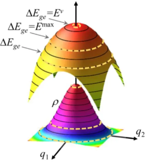
To understand the origin of the shift, consider the following simple two-modes/two-states analytical model. The two two-modes/two-states are separated by a vertical transition energy E . For v
each state, the potential energy surface is supposed to be given by two uncoupled harmonic and degenerated potentials in the coordinates q1 and q2, with the ground and excited states
sharing the same equilibrium geometry, but with different angular frequencies g and e. Without losing generality, the energy of the ground-state equilibrium geometry is assumed to be zero. Thus, the ground- and excited-state potential energies are given as [23]
(
)
(
)
2 2 2 1 2 2 2 2 1 2 1 , 2 1 . 2 g g v e e E q q E E q q = + = + + (1)where is the reduced mass. The resonance condition is
(
)
(
2 2)(
2 2)
1 2 1 0. 2 v ge P P e g E E E E q q − = − + − + = (2)In a semiclassical approximation, the spectrum is given by
(
1, 2)
(
eg(
1, 2)
p)
1 2k q q g E q q E dq dq
=
− (3)where is the distribution of geometries in the ground state, and g is a line-shape function satisfying the resonance condition in Eq. (2). k is a constant, which includes the oscillator strength between the two states (Condon approximation). If is given by a Wigner distribution for the quantum harmonic oscillator,
6
(
)
(
(
2 2)
)
1, 2 exp 1 2 , , g q q q q = − + (4)and the line-shape function is taken as a normalized Gaussian function with arbitrary width w,
( )
22 1 exp x , g x w w = − (5) we obtain(
2 2)
(
)
(
2 2)(
2 2)
2 1 2 1 2 1 2 3/2 2 1 1 exp . 2 v p e g k q q E E q q dq dq w w = − + − − + − +
(6)w is assumed to be much narrower than the band width, and in the limit when it tends to zero, g converges to a Dirac delta function.
In polar coordinates
(
q1=Rcos( )
,q2 =Rsin( )
)
, Eq. (6) becomes(
)
(
)
2 2 2 2 2 3/2 2 1 1 exp , 2 v p e g k R E E R RdRd w w = − − − + −
(7)which can be analytically integrated to give
(
)
(
)
2 2 2 2 2 exp 1 v p 1 1 v p , k w A w A E E erf E E A A w A w = − + − + + − (8) where(
2 2)
. e g g A − = (9)The maximum of this spectral band happens for the photon energy Emax satisfying
/ P 0
d dE = . If we expand this derivative to the first order in E around p v
E , we obtain the shift
(
2 2)
max . 2 g e v g E E − − = (10)7 Because upon excitation the bond is loosened, it implies that e g and, therefore,
max
.
v
E E This means that the band maximum is redshifted in relation to the vertical excitation.
Illustration of the 2-modes/2-states analytical model. The upper surface shows the potential energy difference Ege while the bottom surface illustrates the Wigner distribution in the ground state. The
ge P
E E
=
dashed curves indicate isoenergetic curves satisfying the resonance condition .
With this simple model, it is easy to understand the origin of the shift. For a certain photon energy EP, the spectral intensity in Eq. (3) is determined by both the ground state population on the isoenergetic line satisfying the resonance condition and the length of this line. In this model, this line is merely a circle, but it is a hyperline in general multidimensional cases. In one limiting case, the ground state population is maximal (q1 = q2 = 0) but the line
length is too short, yielding a low spectral intensity. In the case of excited and ground states sharing the same equilibrium geometry, this limit happens at Ev. In the other limiting case, the curve length tends to infinite (q1 = q2 → ∞), but the ground state population is null, also yielding
a minimal intensity. Between the two extremes, the band maximum occurs at Emax, with optimal length and population values, which is proportional to the difference between the squared frequencies of the excited and ground states (Eq. (10)).
Although there are no analytical results for multidimensional, realistic cases, this dependence of the shift on the difference of the squared frequencies seems to be general. For instance, as mentioned in the Introduction, Avila Ferrer et al. [3] proposed to compare vertical excitations to the first-moment M1 of the absorption band to approximately account for the shift effect. They recall that the M1 can be analytically computed for harmonic ground and
8 excited states in the Franck-Condon approximation, with the excited state built in the vertical Hessian approach. In this model, the shift between the vertical excitation and M1 is [24]
(
2 2)
2 , , , 1 , coth , 4 2 g r e r g r v r g r B E M k T − − =
(11)where kB is the Boltzmann constant, T is the temperature, and r runs over the normal modes. In the limit of low temperature and two degenerated normal modes, this expression yields the shift given by Eq. (10).
Note yet that the shift seems to be a multidimensional phenomenon. We have not been able to find an analytical expression for the shift in a single-dimensional model, but numerical estimates showed that in such a case the shift is a function of the width w, and it tends to zero for small w. In the limit of a Dirac delta function (w = 0), the band of the single-dimensional model is peaked at the vertical excitation [23].
Analysis of the shift with model systems
To get further numerical insights into the origin of the shift, we simulated the absorption spectrum of a model system with few vibrational modes using the nuclear ensemble approach. The advantage of working with such low-dimensionality systems is that we can systematically control the values of key parameters to verify their impact on the spectrum.
The model systems are composed of two harmonic potentials representing the ground and the first excited states. The simplest model contains a single vibrational mode (1V) with ground-state frequency g and excited-state frequency given by e2/ g2 = , where is a constant. The potential energies of the ground and excited states are
(
)
2 2 2 2 1 2 1 2 g g v e g E q E E q d = = + − (12)In the simulations, E =v 4.08 eV (0.15 au), =1.0 amu (1823 au) and g =1500 cm
-1 (0.0068 au). To compute the spectrum, 50,000 geometries were sampled from a Wigner
9 As expected for the one-dimensional model, the results do not show any shift for small
w.
We extended the 1V model into three vibrational modes (3V), with ground-state frequencies g1 = 1800, g2 = 1500, and g3 = 1000 cm-1; frequency-changing parameters 1,
2, and 3; and displacements d1, d2, and d3. All other parameters were kept at the same values
as in the 1V model.
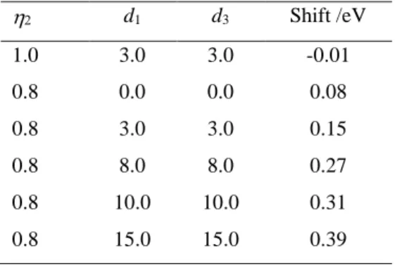
The results for the shift with the 3V model are given in Table 1. Now, we see that displacements without a frequency change lead to a negligible shift. For 2 = 0.8, as the
displacements of the other two modes increase, the shift increases, too. This result tells that although the displacement does not cause the shift, it modulates the shift value.
Table 1. Numerical simulations of the shift (eV) between the vertical excitation and the band maximum for a model with three vibrational modes, considering a shift between the ground and excited-state frequencies (given by ) and a displacement di (au) between the modes. All results with 1 = 3
= 1.0 and d2 = 10 a.u. d1 d3 Shift /eV 1.0 3.0 3.0 -0.01 0.8 0.0 0.0 0.08 0.8 3.0 3.0 0.15 0.8 8.0 8.0 0.27 0.8 10.0 10.0 0.31 0.8 15.0 15.0 0.39
Benchmark of shift values
Based on the vertical excitations and the results from the nuclear ensemble simulations, we investigated the shift between the vertical transition energy Ecalcv and the band maximum
max
calc
E in the 28 molecules of the Mülheim dataset. Figure 4 illustrates these simulations for three molecules—cyclopropene, pyridine, and pyrimidine (molecules 5, 13, and 15 in Figure 2).
10
Comparison between the nuclear ensemble spectrum simulation (solid black) and the vertical excitations (sticks) for (top) cyclopropene, (middle) pyridine, and (bottom) pyrimidine. The fitting of the nuclear ensemble result is shown as a dashed red curve. The Gaussian function components of the fitting, corresponding to the sub-bands of each vertical excitation, are shown as well.
For energies in eV and absorption cross section in Å2.molecule-1, the spectrum convolution can be written as (see derivation in Appendix A)
( )
( )2/ 2 0.619 , v i i i E E i A i i f E n e = − − +
(13)where n is the refractive index, and E , iv fi, , and i i are, respectively, the vertical excitation, oscillator strength, shift, and width of band i. We used this expression to fit the simulated spectra. In the fitting process, E and iv fi were kept fixed, and we got , and i i. In some cases, the oscillator strength was also optimized to improve the fitting (see Supporting Information).The number of Gaussian functions used to fit each spectrum was determined by the number of vertical excitations with considerable oscillator strength in the spectral region of interest. Thus, for some bands, several Gaussian functions (up to five) were needed. This is the case of cyclopropene shown in Figure 4-top (which required three Gaussian functions) and of
5 6 7 8 0.0 0.1 0.2 4.0 4.5 5.0 5.5 6.0 0.0 0.1 3.5 4.0 4.5 5.0 5.5 6.0 0.0 0.1 Cyclopropene ( Å 2 .m o le cu le − 1 ) Pyridine Energy (eV) Pyrimidine
11 pyridine in Figure 4-middle (two Gaussian functions). Other bands, like those in pyrimidine (Figure 4-bottom), required only one Gaussian function.
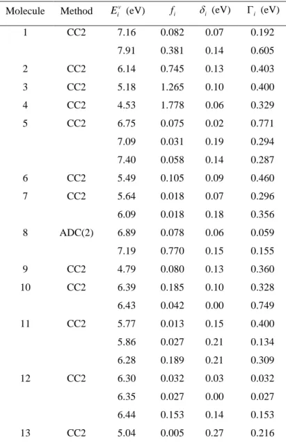
The shift results for all molecules are collected in Table 2. All fitted parameters are given in the Supporting Information. As shown in this table, for all 28 molecules we observe sub-bands with a redshift between the band maximum and the vertical excitation. The shift varies from zero to 0.4 eV; its mean value is 0.11 eV, and the standard deviation is 0.08 eV. As expected, the shift value does not show any correlation either with E or with iv fi.
Table 2. Vertical excitation energy ( v i
E in eV) and oscillator strengths (fi) for all molecules
28 molecules in the Mülheim dataset in the fitted spectral region. The peak of each Gaussian sub-band is redshifted by (eV) from i v
i
E . The width of the sub-band is i (eV). Molecules are numbered as
in Figure 2.
Molecule Method Eiv (eV) fi i (eV) i (eV)
1 CC2 7.16 7.91 0.082 0.381 0.07 0.14 0.192 0.605 2 CC2 6.14 0.745 0.13 0.403 3 CC2 5.18 1.265 0.10 0.400 4 CC2 4.53 1.778 0.06 0.329 5 CC2 6.75 7.09 7.40 0.075 0.031 0.058 0.02 0.19 0.14 0.771 0.294 0.287 6 CC2 5.49 0.105 0.09 0.460 7 CC2 5.64 6.09 0.018 0.018 0.07 0.18 0.296 0.356 8 ADC(2) 6.89 7.19 0.078 0.770 0.06 0.15 0.059 0.155 9 CC2 4.79 0.080 0.13 0.360 10 CC2 6.39 6.43 0.185 0.042 0.10 0.00 0.328 0.749 11 CC2 5.77 5.86 6.28 0.013 0.027 0.189 0.15 0.21 0.21 0.400 0.134 0.309 12 CC2 6.30 6.35 6.44 0.032 0.027 0.153 0.03 0.00 0.14 0.032 0.027 0.153 13 CC2 5.04 0.005 0.27 0.216
12 5.32 0.032 0.05 0.278 14 CC2 4.18 5.14 0.006 0.085 0.14 0.05 0.213 0.229 15 CC2 4.44 5.52 6.11 0.006 0.030 0.004 0.07 0.11 0.15 0.395 0.262 0.323 16 CC2 3.83 5.39 0.005 0.018 0.08 0.06 0.286 0.359 17 CC2 4.80 0.016 0.06 0.422 18 CC2 5.24 0.056 0.09 0.364 19 CC2 6.38 0.022 0.05 0.128 20 CC2 5.74 0.031 0.08 0.226 21 ADC(2) 5.33 0.593 0.14 0.393 22 CC2 6.13 6.55 6.71 7.23 7.53 0.028 0.021 0.064 0.029 0.337 0.05 0.17 0.01 0.10 0.05 0.349 0.215 0.251 0.241 0.500 23 CC2 5.77 6.36 6.88 7.26 7.60 0.032 0.019 0.019 0.206 0.056 0.00 0.03 0.19 0.09 0.00 0.452 0.239 0.241 0.421 0.240 24 CC2 5.77 6.36 6.76 7.19 7.48 0.026 0.020 0.014 0.189 0.027 0.02 0.08 0.00 0.16 0.00 0.399 0.247 0.259 0.394 0.192 25 CC2 4.68 5.57 0.050 0.137 0.08 0.18 0.412 0.391 26 ADC(2) 5.10 6.10 6.19 0.205 0.028 0.048 0.18 0.41 0.20 0.418 0.275 0.254 27 CC2 5.34 6.30 0.182 0.068 0.17 0.23 0.344 0.430 28 ADC(2) 5.13 5.19 0.247 0.059 0.17 0.00 0.357 0.569
The current results confirm that the redshifts are a common feature shared by many molecules. 80% of the sub-bands presented shifts equal or superior to 0.05 eV. Therefore, it
13 seems that the standard practice of comparing computed vertical excitations to the experimental band maxima should be reconsidered. Ideally, we should compare the experimental band maximum to the calculated band maximum. If only vertical excitations are known (as it is usually the case), a simple estimate of the band maximum is given by Ecalcmax =Eiv− , where
0.1
= eV is the mean value of our benchmark. This point is further elaborated in the next section, where we discuss a specific example.
The fitting of the simulated spectra yielded the sub-band width i as a side product. Their values are also given in Table 2. The minimum width is 0.03 eV and the maximum 0.77 eV. The mean value is 0.32 eV, and the standard deviation is 0.14 eV.
Accounting for the shifts in spectrum convolutions
The parameters in the simple spectrum convolution defined in Eq. (13) are illustrated in Figure 1. This equation is often used to make simple spectrum simulations from vertical excitation energies and oscillator strengths calculated at the equilibrium geometry. In such applications, the width is either taken as an arbitrary value common to all bands (based on our benchmark, we recommend to employ = 0.3 eV) or fitted to experimental values.
Note that the area under each sub-band in Eq. (13) is proportional to the oscillator strength of the corresponding vertical excitation. Nevertheless, it is still common in the literature to find spectrum convolutions taking the oscillator strength as the height of the sub-band. Such a procedure, however, should be avoided, as it does not bear the right functional form fi /i and delivers spectra in arbitrary units.
Figure 5 shows the absorption cross-section of pyrimidine in the gas phase. Compared to the experimental spectrum from Ref. [25], the simulations deliver satisfactory results. The intensity and position of the two bands are semi-quantitively described. Neither the spectrum convolution nor the nuclear ensemble can describe the vibrational resolution of the bands. Nevertheless, in the nuclear ensemble, the band envelope is a result of the simulation, while in the simple convolution, it is assumed to be a sum of Gaussian functions with an arbitrary width . Naturally, there is a large difference in the computational effort invested in the two methods. While the Gaussian convolution only demands the calculation of vertical excitation energies and oscillator strengths for the ground-state equilibrium geometry, the nuclear ensemble needs hundreds of such calculations; in the present case, 500 single points.
14
Absorption cross section for pyrimidine in the gas phase. Spectrum convolutions based on Eq. (13) with the same width value for all sub-bands (0.3 eV). Nuclear ensemble spectra computed with 500 points. Experimental data from Ref. [25].
If now we turn our attention to the spectrum convolutions and the nuclear ensemble results in Figure 5, we can clearly see the effect of the shift. With =0, the convolution is blueshifted compared to the nuclear ensemble band. A significantly better agreement is obtained when a shift =0.1 eV is uniformly applied to both bands.
Experimentally, the high-energy band is peaked at 5.2 eV [25]. The vertical excitation energy computed with CC2 is at 5.52 eV, 0.32 eV above the experimental value. However, as we have been discussing, we should preferentially compare the estimated band maximum to the experimental result. The band maximum computed with the nuclear ensemble, still with CC2, is at 5.43 eV, therefore, 0.23 eV above the experimental value. A simpler estimate of the band maximum is obtained by computing Eiv− , where =0.1 eV, the mean shift value obtained from our benchmark. In this case, the band maximum estimate is 5.42 eV, 0.22 eV above the experimental value.
Conclusion
It is well established in the literature that band maxima of absorption spectra are redshifted in comparison to the corresponding vertical excitations by values reaching up to = 0.2 eV (assuming that both are computed with the same electronic-structure method). Using an analytical model and numerical estimates from low-dimensionality model systems, we determined that these shifts are primarily caused by the frequency change between the ground
3.5 4.0 4.5 5.0 5.5 6.0 0.00 0.02 0.04 0.06 0.08 Experimental Nuclear ensemble Convolution = 0 eV Convolution = 0.1 eV ( Å 2.m o le cu le − 1)
15 and the excited states in multidimensional systems. The geometry displacement between the ground- and excited-state minima does not cause the shift but may affect its value. Nuclear ensemble simulations for a dataset of 28 small organic molecules completed this analysis by delivering a benchmark of shift values. The mean value of the shift calculated over 60 transitions is 0.11 eV with 0.08 eV standard deviation. The mean value of the band width is 0.32 eV with 0.14 eV standard deviation.
Despite the availability of highly accurate methods for spectrum simulations, it is likely that the workhorse method for routine estimation of the one-photon absorption of molecules will remain the simple spectrum convolution of vertical excitations. Based on the results presented in this paper, we recommend that in such convolutions the shift should be systematically taken into consideration in the comparison between the experimental band maximum and computed vertical excitations. This can be done, for instance, following the suggestion of Ref. [3] of comparing the vertical excitation to the M1 moment of the experimental band. Alternatively, it can be simply done by estimating the band maximum by redshifting the vertical excitation by 0.1 eV, the mean value of our benchmark.
Appendix A.
Derivation of Eq. (13)
Experimentally, the oscillator strength of an absorption band i is given as [26]
( )
( )
3 2 10 ln 10 , e i i A m c f d N e n =
(14)where me is the electron mass, c is the speed of the light, NA is the Avogadro’s number, e is the electron charge, and n is the refractive index (CGS units).
i is the molar absorbance (or extinction coefficient). The integral is done over the absorption frequency . Supposing that the band has a Gaussian shape with maximum imax at imax, and width
i, the integral is( )
( max)2/ 2 max max . i i i d i e d i i = − − =
(15)Thus, the oscillator strength is
( )
3 max 2 10 ln 10 . e i i i A m c f N e n = (16)16
( )
( )
( )( )
( ) 2 max 2 2 max 2 / max 2 / 3 . 10 ln 10 i i i i i i i i A i i e i e N e n f e m c − − − − = = =
(17)The absorption cross section is [26]
( )
( )
( )
( max)2 2 3 2 / 10 ln 10 . i i A i i e i N e n f e m c − − = =
(18)It is convenient to express the absorption cross section in terms of the absorption energy
( )
3/2 2 ( max)2 2 / 2 , i i E E i i e i e n f E e m c = − −
(19)where i is the energy width of the band and Eimax its energy maximum. As usual, is the reduced Planck constant.
To account for the shift between the band maximum Eimax and the vertical excitation v
i
E , it is convenient to introduce an energy-shift parameter i to account for this effect:
max
. v
i i i
E =E − (20)
Replacing this equation in Eq. (17) leads to (CGS units)
( )
3/2 2 ( )2 2 / 2 . v i i i E E i i e i e n f E e m c = − − +
(21)For energies in eV and absorption cross section in Å2.molecule-1, it results in Eq. (13).
From this result, the molar absorbance is
2 --1 1 -1 5 Å .molecu . M cm 3.82353 1 le 0 = − (22)
17
Acknowledgments
The authors thank the support of the Excellence Initiative of Aix-Marseille University (A*MIDEX) and the project Equip@Meso (ANR-10-EQPX-29-01), both funded by the French Government “Investissements d’Avenir” program. M.B. and R.M. thank the European Research Council (ERC) Advanced grant SubNano (Grant agreement 832237). M.B. and J.M.T. thank the FetOpen grant BoostCrop (Grant agreement 828753).
References
1. Bomble YJ, Sattelmeyer KW, Stanton JF, Gauss J (2004) On the vertical excitation energy of cyclopentadiene. J Chem Phys 121 (11):5236-5240
2. Barbatti M, Aquino AJA, Lischka H (2010) The UV absorption of nucleobases: semi-classical ab initio spectra simulations. Phys Chem Chem Phys 12 (19):4959-4967
3. Avila Ferrer FJ, Cerezo J, Stendardo E, Improta R, Santoro F (2013) Insights for an Accurate Comparison of Computational Data to Experimental Absorption and Emission Spectra: Beyond the Vertical Transition Approximation. J Chem Theory Comput 9 (4):2072-2082. doi:10.1021/ct301107m
4. Zobel JP, Nogueira JJ, Gonzalez L (2017) The IPEA dilemma in CASPT2. Chem Sci 8 (2):1482-1499. doi:10.1039/C6SC03759C
5. Barton D, König C, Neugebauer J (2014) Vibronic-structure tracking: A shortcut for vibrationally resolved UV/Vis-spectra calculations. J Chem Phys 141 (16):164115. doi:10.1063/1.4898665
6. Reddy CS, Prasad MD (2016) A Gaussian Wave Packet Propagation Approach to Vibrationally Resolved Optical Spectra at Non-Zero Temperatures. J Phys Chem A 120 (16):2583-2590. doi:10.1021/acs.jpca.6b00308
7. Baiardi A, Bloino J, Barone V (2013) General Time Dependent Approach to Vibronic Spectroscopy Including Franck–Condon, Herzberg–Teller, and Duschinsky Effects. J Chem Theory Comput 9 (9):4097-4115. doi:10.1021/ct400450k
8. Segarra-Martí J, Segatta F, Mackenzie TA, Nenov A, Rivalta I, Bearpark MJ, Garavelli M (2020) Modeling multidimensional spectral lineshapes from first principles: application to water-solvated adenine. Faraday Discuss. doi:10.1039/C9FD00072K
9. Reddy CS, Prasad MD (2015) Finite temperature vibronic spectra of harmonic surfaces: a
time-dependent coupled cluster approach. Mol Phys 113 (19-20):3023-3030.
18 10. Santoro F, Improta R, Lami A, Bloino J, Barone V (2007) Effective Method to Compute Franck-Condon Integrals for Optical Spectra of Large Molecules in Solution. J Chem Phys 126 (8):084509. doi:10.1063/1.2437197
11. Charaf-Eddin A, Cauchy T, Felpin F-X, Jacquemin D (2014) Vibronic spectra of organic electronic chromophores. RSC Advances 4 (98):55466-55472. doi:10.1039/C4RA10731D 12. Crespo-Otero R, Barbatti M (2012) Spectrum Simulation and Decomposition with Nuclear Ensemble: Formal Derivation and Application to Benzene, Furan and 2-Phenylfuran. Theor Chem Acc 131 (6):1237. doi:10.1007/s00214-012-1237-4
13. Schreiber M, Silva-Junior MR, Sauer SPA, Thiel W (2008) Benchmarks for electronically excited states: CASPT2, CC2, CCSD, and CC3. J Chem Phys 128 (13):134110
14. Christiansen O, Koch H, Jorgensen P (1995) The 2nd-Order Approximate Coupled-Cluster Singles and Doubles Model CC2. Chem Phys Lett 243 (5-6):409-418
15. Hättig C, Köhn A (2002) Transition Moments and Excited-State First-Order Properties in the Coupled-Cluster Model CC2 Using the Resolution-of-the-Identity Approximation. J Chem Phys 117 (15):6939-6951. doi:Doi 10.1063/1.1506918
16. Dunning Jr. TH (1989) Gaussian Basis Sets for Use in Correlated Molecular Calculations. I. The Atoms Boron Through Neon and Hydrogen. J Chem Phys 90 (2):1007-1023. doi:10.1063/1.456153
17. Schirmer J (1982) Beyond the Random-Phase Approximation: A New Approximation Scheme for the Polarization Propagator. Phys Rev A 26 (5):2395-2416
18. Ahlrichs R, Bär M, Häser M, Horn H, Kölmel C (1989) Electronic-Structure Calculations on Workstation Computers - the Program System Turbomole. Chem Phys Lett 162 (3):165-169
19. Barbatti M, Granucci G, Ruckenbauer M, Plasser F, Crespo-Otero R, Pittner J, Persico M, Lischka H (2018) NEWTON-X: A package for Newtonian Dynamics Close to the Crossing Seam (v. 2.2). Available via the Internet at www.newtonx.org.
20. Barbatti M, Ruckenbauer M, Plasser F, Pittner J, Granucci G, Persico M, Lischka H (2014) Newton-X: A Surface-Hopping Program for Nonadiabatic Molecular Dynamics. WIREs: Comp Mol Sci 4 (8):26-33
21. Mansour R, Barbatti M (2019) Spectra Simulation. Available for download at https://github.com/Ritam19/Spectra-Simulation.git.
22. Band YB, Freed KF (1977) Energy distribution in selected fragment vibrations in dissociation processes in polyatomic molecules. J Chem Phys 67 (4):1462-1472. doi:10.1063/1.435020
19 23. Schinke R (1995) Photodissociation Dynamics: Spectroscopy and Fragmentation of Small Polyatomic Molecules. Cambridge University Press, Cambridge
24. Biczysko M, Bloino J, Santoro F, Barone V (2011) Time-Independent Approaches to Simulate Electronic Spectra Lineshapes: From Small Molecules to Macrosystems. In: Computational Strategies for Spectroscopy. John Wiley & Sons, Inc., pp 361-443. doi:10.1002/9781118008720.ch8
25. da Silva FF, Almeida D, Martins G, Milosavljevic AR, Marinkovic BP, Hoffmann SV, Mason NJ, Nunes Y, Garcia G, Limao-Vieira P (2010) The electronic states of pyrimidine studied by VUV photoabsorption and electron energy-loss spectroscopy. Phys Chem Chem Phys 12 (25):6717-6731. doi:10.1039/b927412j