Setting priors and enforcing constraints on matches for nonlinear registration of meshes.

HAL Id: inserm-00440681

https://www.hal.inserm.fr/inserm-00440681

Submitted on 11 Dec 2009

HAL is a multi-disciplinary open access

archive for the deposit and dissemination of

sci-entific research documents, whether they are

pub-lished or not. The documents may come from

teaching and research institutions in France or

abroad, or from public or private research centers.

L’archive ouverte pluridisciplinaire HAL, est

destinée au dépôt et à la diffusion de documents

scientifiques de niveau recherche, publiés ou non,

émanant des établissements d’enseignement et de

recherche français ou étrangers, des laboratoires

publics ou privés.

Setting priors and enforcing constraints on matches for

nonlinear registration of meshes.

Benoît Combès, Sylvain Prima

To cite this version:

Benoît Combès, Sylvain Prima. Setting priors and enforcing constraints on matches for nonlinear

registration of meshes.. 12th International Conference on Medical Image Computing and

Computer-Assisted Intervention (MICCAI’2009), Sep 2009, Londres, United Kingdom. pp.175-183,

�10.1007/978-3-642-04271-3_22�. �inserm-00440681�

Setting Priors and Enforcing Constraints on

Matches for Nonlinear Registration of Meshes

Benoˆıt Comb`es and Sylvain Prima

INSERM, U746, F-35042 Rennes, France INRIA, VisAGeS Project-Team, F-35042 Rennes, France

University of Rennes I, CNRS, UMR 6074, IRISA, F-35042 Rennes, France [bcombes,sprima]@irisa.fr, http://www.irisa.fr/visages

Abstract. We show that a simple probabilistic modelling of the regis-tration problem for surfaces allows to solve it by using standard clus-tering techniques. In this framework, point-to-point correspondences are hypothesized between the two free-form surfaces, and we show how to specify priors and to enforce global constraints on these matches with only minor changes to the optimisation algorithm. The purpose of these two modifications is to increase its capture range and to obtain more realistic geometrical transformations between the surfaces. We conclude with some validation experiments and results on synthetic and real data.

1

Introduction

In medical image analysis, nonlinear registration is a key tool to study the nor-mal and abnornor-mal anatomy of body structures. It allows to spatially nornor-malise different subjects in a common template, to build the average anatomy in a pop-ulation and to assess the variance about this average, and ultimately to perform group studies via statistical analyses. Many methods have been dedicated to deal with grey level volumes directly, while others have been devised to tackle surfaces representing anatomical structures (e.g. after segmentation from MRI or CT) [1]. The last approach allows a more focused analysis of structures of interest, and is the topic of our paper. In Section 2 we show that a simple proba-bilistic modelling of the registration problem allows to solve it by using standard clustering techniques. In this framework, point-to-point correspondences are hy-pothesized between the two free-form surfaces, and we show how to specify priors (Section 3) and to enforce global constraints (Section 4) on these matches with only minor changes to the optimisation algorithm. This extends our previous work on the same problem [2]. The purpose of these two modifications is to in-crease its capture range and to obtain more realistic geometrical transformations between the surfaces. We conclude with some validation experiments and results on synthetic and real data (Section 5).

2

Surface Registration as a Clustering Problem

The problem of interest in this paper is to find the transformation T best super-posing two free-form surfaces X and Y (represented by point clouds or meshes).

A convenient probabilistic viewpoint on this classical problem is to consider the surface Y as a noised version of T (X). If we note Y = (yj)j=1... card(Y )

and X = (xk)k=1... card(X), and if we hypothesize an isotropic Gaussian noise,

a simple way to formulate this viewpoint is to assume that each sample yj has

been drawn independently from any one of card(X) possible 3-variate normal distributions with means T (xk) and covariance matrices σ2I (with σ unknown).

This way, the registration problem becomes a clustering problem, whose chal-lenge is i) to find the label of each point yj, i.e. the one out of card(X) possible

distributions from which yj has been drawn, and ii) to estimate the parameters

of these card(X) distributions. The connection between registration and cluster-ing becomes clear when one realises that i) actually amounts to match each point yj in Y with a point xk in X, while ii) simply consists in computing T given

these matches. This viewpoint is extremely fruitful, as it allows one to refer to classical clustering techniques and especially the maximum likelihood principle to solve the registration problem. Two different paradigms have been especially followed in this context [3]. Let us introduce some notations first:

∀k ∈ 1... card(X), pk(.; T ) = N (T (xk), σ2I)

∀j ∈ 1... card(Y ), ∀k ∈ 1... card(X), zjk= 1 if yj comes from pk(.; T ), 0 else

In the Classification ML (CML) approach, one tries to find the indicator variables zjk and the parameter T so as to maximise the criterion CL [4]:

CL = Y

yj∈Y

Y

xk∈X

[pk(yj; T )]zjk (1)

The problem is typically solved by the Classification EM (CEM) algorithm [5], which can be shown to find an at least local maximum of the criterion CL and proceeds as follows, in an iterative way, starting from an initial value ˜T :

EC-step:∀j, ˜zjk= 1 if k maximises pk(yj; ˜T ), 0 else

M-step: ˜T = arg minTPjkz˜jk||yj− T (xk)||2

In other words, the Expectation-Classification (EC) step consists in match-ing each point yj of Y with the closest point in ˜T (X), while the Maximisation

(M) step consists in computing the transformation best superposing these pairs of matched points. In case T is a rigid-body transformation, this is nothing else than the popular ICP algorithm [6].

In the ML approach, the indicator values zjk are no longer considered as

unknown quantities to estimate, but rather as hidden/unobservable variables of the problem. This is actually a drastic and fundamental change of viewpoint, as the focus is no longer on assigning each yj to one of the distributions pk

but rather on estimating the parameters of the Gaussian mixture made of these distributions. If we involve priors πjk on the indicator variables (∀j, k, 0 < πjk<

1, and ∀j,P

kπjk= 1), the likelihood then simply writes [7]:

L = Y

yj∈Y

X

xk∈X

In essence, the prior πjk conveys the probability that the point yj comes

from the distribution pk without knowing anything else. The criterion L can

be maximised by using the popular EM algorithm, which converges to an at least local maximum of the likelihood [8]. If we consider the priors πjk as known

beforehand and if we introduce the notation γjk as the posterior probability of

the hidden indicator variable zjk to be equal to 1, the EM algorithm writes:

E-step: ˜γjk=

πjkexp[−||yj− ˜T (xk)||2/(2σ2)]

P

iπjiexp[−||yj− ˜T (xi)||2/(2σ2)]

M-step: ˜T = arg minTPjkγ˜jk||yj− T (xk)||2

To our knowledge, Granger & Pennec [9] were the first to formulate the problem this way, and they proposed the so-called EM-ICP as a simplified ver-sion of the previous algorithm for rigid-body registration, where the priors πjk

were considered as uniform. They noted that the parameter σ, which is not esti-mated in this framework, acts as a scale parameter, and that it can be given an initial value and decreased throughout the iterations for improved performances. Interpretation & Extensions: Intuitively, the EM approach is a fuzzy version of the CEM. It appears clearly from the iterative formulas of both algorithms that the classification likelihood is an “all-or-nothing” version of the likelihood, leading to a “bumpier” and harder-to-maximise criterion, something that is well known by those who are familiar with the ICP algorithm. Note that the ML formulation and the EM algorithm lead to the same iterative formulas that would have resulted from the addition of a barrier function on the indicator variables in the ICP criterion [10]. This formalism is not limited to rigid-body transformations, and can be easily used for any T , the challenge being to choose T such that the M-step remains tractable. In particular, the ML estimation can be easily turned into a MAP problem with only slight modifications to the optimisation scheme, as shown by Green [11]. This allows to view T as a random variable, on which priors (acting as regularisers on T ) can be easily specified. Different choices have been proposed for T and associated priors in this context, such as the thin plate splines [10] or locally affine transformations [12]. If p(T ) is a prior of the form p(T ) ∝ exp(−αR(T )) then the optimal transformation can be found using the MAP principle (also termed penalised ML) and the EM algorithm with only a slight modification to the M-step (addition of αR(T )).

3

Setting Priors on Matches

Most works in this context have been focused on designing transformations and related priors allowing to i) compute realistic deformations between the two sur-faces and ii) keep the M-step tractable. Much little has been done to enforce similar constraints on the matches (E-step). Dropping the priors πjk, as done

in the ICP of Besl & McKay or the EM-ICP of Granger & Pennec amounts to say that the posteriors γjk are only estimated using the spatial distance between

the points yj and T (xk) (E-step). This is unsatisfactory, for two reasons. First,

turn depends on the previous estimation of γjk and so on. This chicken-and-egg

problem limits the capture range of the algorithm, which is likely to converge to a bad solution if no good initial T is given. Second, in medical imaging it is difficult to design a physical model T capturing the expected deformation be-tween two structures. Thus the global maximiser of the ML criterion is likely not to be realistic. By specifying relevant priors πjk, we provide a way to partially

alleviate these two limitations. First, it allows to introduce additional informa-tion on matches independent of the transformainforma-tion and thus to compute reliable posteriors even for a bad initial estimate of T . Second, it allows to modify the criterion in a way that its global maximiser is a more realistic transformation.

3.2 Building Priors on Matches

In this section we show how to design the priors πjk to encode very

hetero-geneous types of a priori knowledge on the matches, such as “two points with similar curvatures are more likely to be matched than others” as well as knowl-edge of the labels of structures in the objects to be matched (e.g. gyri/sulci in cortical registration). In practice, we choose to design π = (πjk) such that

πjk ∝ exp(−βc(yj, xk)) where c : X × Y → IR+ conveys the cost of matching

points yjand xk, independently of T . The parameter β > 0 weighs the influence

of πjk over ||yj− T (xk)|| during the E-step. Depending on the information to

encode (continuous value or label), we propose two approaches to build c. Using descriptors: c can be computed via the comparison between continuous values (or vectors) d(x) describing the surface around the considered points. To account for potential inaccuracies on d(.), we define the measure as: cd_(y

j, xk) =

0 if ||d(yj) − d(xk)|| < τ ; = penalty > 0 else. To the best of our knowledge, there

exists no descriptor invariant to any nonlinear transformation. However, one can use some descriptors invariant to more constrained transformations (Fig. 1, left): – the shape index sh(x) [13] that describes the local shape irrespective of the

scale and that is invariant to similarities

– the curvedness cu(x) [13] that specifies the amount of curvature and that is invariant to rigid-body transformations

– the (normalised) total geodesic distance tgd(x) [14] that is invariant to isome-tries in the shape space (including non-elastic deformations).

Using labels: c can be computed via the comparison between labels on points (cortical sulci/gyri). We define: c(yj, xk) = 0 if points j and k have compatible

labels; = penalty > 0 else. In practice, we extract the crest lines from both meshes as they constitute salient features. Each point is given a label depending on whether it belongs to a crest line or not. Then, we define ccrest(yj, xk) = 0 if

yj and xk have the same label and c(yj, xk) = penalty else.

Mixing the two approaches: In practice, we choose to mix the previous four sources of information to build the function c: c(yj, xk) = a1csh(yj, xk) +

a2ccu(yj, xk) + a3ctgd(yj, xk) + a4ccrest(yj, xk) with a1+ a2+ a3+ a4= 1.

Param-eters aiallow to weigh the different terms. Their values is application-dependent

Fig. 1. Left: Mapping of descriptor values: From left to right: curvedness, shape index and total geodesic distance on two lateral ventricles. Homologous anatomical landmarks yield qualitatively the same descriptor values. Right: point-based matching (top) vs line-based matching performed by our algorithm (bottom).

3.3 Efficient Implementation

In practice, we do not consider all points during the computation of γjk(E-step).

For that, we consider pk(.; T ) as a truncated Gaussian pdf with cut-off distance

δ. This allows to reduce the computational burden (by the use of a kd-tree) and increase robustness. It can be shown that our algorithm still converges to an at least local maximum of the new (truncated) criterion. The E-Step becomes:

initialise γ = (γjk) to the null matrix

∀xk ∈ X

S = {yj ∈ Y such that ||yj− ˜T (xk)||2< δ} (using a kd-tree)

∀yj ∈ S

γjk= exp(−(||yj− ˜T (xk)||2/(2σ2) + βc(yj, xk)))

∀j, ∀k, ˜γjk= γjk/Plγjl (normalisation)

Moreover, we choose to initialise α (regularisation weight), σ (scale parame-ter) and β (prior weight) with high values and reduce them throughout iterations.

4

Enforcing Global Constraints on Matches

In the formalism presented so far, the matches in the E-step are performed on an individual basis without any global constraint such as one-to-one matches for instance. Another desirable global constraint is that some geometrical relation-ships between points in Y should be preserved between their correspondences in X. Thus if we consider each crest line in Y as a set of ordered points, then their correspondences must i) lie on the same crest line in X and ii) be ordered in the same way (up to the orientation of the line) (Fig. 1 right). To enforce these two constraints, let us introduce some notations first. Let L and M be the sets of crest lines of Y and X, each crest line being defined as a set of ordered points. Let u = (ulm_{) be a block matrix whose lines (resp. columns) correspond}

to the concatenated crest lines of Y (resp. X). Then ulm

jk is the indicator variable

ulm

jk = 1 iff yj in crest line l corresponds to the point xk in crest line m. The two

constraints i) and ii) are specified as follows: the submatrix ulm _{is either null}

(the line l does not match with the line m) or contains one 1 per line, with the 1s drawing a “staircase” going to the left or to the right, all “steps” of the staircase having potentially different widths and different heights. Then we propose to maximise the following criterion over T and u having this staircase structure:

L−CL =   Y yj∈Y \L X xk∈X\M πjkpk(yj|T ) × Y l∈L Y yj∈l X xk∈m [pk(yj|T )]u lm jk  ×p(T ) (3)

This criterion is an hybrid between the classification likelihood and the like-lihood approaches. Introducing u only modifies the E-step of the algorithm, in which u and γ can be estimated independently. The algorithm becomes:

E-Step: compute ˜γ as before

∀l, compute ˜ulm _{respecting the staircase structure}

and maximisingQ yj∈l P xk∈m[pk(yj| ˜T ) ˜ ulm jk]

M-Step: ˜T = arg minTPyj∈Y \L,xk∈X\M˜γjk||yj− T (xk)||

2 +P l∈L P yj∈l,xk∈mu˜ lm jk||yj− T (xk)||2+ αR(T )

To our knowledge, an exhaustive search is the only way to maximise the proposed criterion over u. Instead, we propose to design an heuristic algorithm to do so, that extends the one proposed by Subsol [15] and consists of two steps: i) finding the crest line m ∈ M that corresponds to each l ∈ L and ii) starting from different initial potential matches and assigning iteratively each point yj∈ l

to a point xk ∈ m by keeping the staircase structure of the submatrix ulm.

5

Experiments & Results

In the following we choose to adopt a locally affine regularisation [12] (with only the translational part) because of its ability to perform efficiently (∼ 7min) on large datasets (∼ 50K points).

5.1 Experiments on Synthetic Data

Generation of ground truth data. We first segment a structure X (typically, a pair of lateral ventricles or caudate nuclei, giving surfaces of about 10K points, itksnap.org) from a 3T T1-weighted brain MRI of a healthy subject. Then Y is generated from X by applying a random thin plate spline transformation [2]. Then, we add a uniform Gaussian noise of std 0.5 mm on each point of the deformed surface and remove groups of adjacent vertices to generate holes. This way we generate ground truth pairs of 100 ventricles and 100 caudate nuclei. Evaluation. We evaluate the error by computing the mean distance between homologous points after registration using different strategies. The results are reported in Tab. 1 and an example is displayed in Fig. 2. They show the strong added value of using priors. The error is further reduced when using constraints, which ensure that the ordering of the points on the lines is kept unchanged, and thus help the algorithm to obtain anatomically coherent matches elsewhere.

5.2 Experiments on Real Data

In a first experiment, we choose X and Y as two different lateral ventricles and manually extract a set of 8 anatomical landmarks common to X and Y . We then

no prior/no constraint prior/no constraint prior/constraint ventricle 2.19 ± 0.82 1.43 ± 0.91 1.39 ± 0.93 caudate nuclei 1.54 ± 0.43 1.04 ± 0.57 0.98 ± 0.56

Table 1. Experiments on synthetic data (stats). Mean and std (mm) of the reg-istration error for the 100 ventricles and 100 caudate nuclei by varying the parameters.

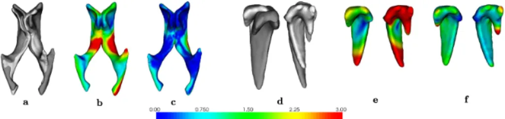
Fig. 2. Experiments on synthetic data. From left to right: Experiments on two different structures: ventricles and caudate nuclei. a) and d) original and deformed; b) and e) mapping of registration error (mm) without using prior/constraint; c) and f) mapping of registration error using prior/constraint.

apply a random affine transformation A to Y , register A(Y ) to X with and with-out using priors/constraints, and evaluate the registration error on landmarks. We perform this experiment 100 times (but we display only 10 on Fig. 3 for better clarity). We observe a mean error of 1.73 ± 1.24mm with the priors/constraints and 2.55 ± 2.46mm without (Fig. 3, left). In a second experiment, we segment the brain from T1-weighted MRI data of two healthy subjects (300,000 points, brainvisa.info), and we extract four sulcal fundus beds (using our algorithm for crest lines) and label them manually for each subject. Then we register the two surfaces with and without using priors/constraints. The distance between the homologous sulci after registration is used as a quality metric. It is evaluated to be 3.3mm in the first case and 6.8mm in the second (Fig. 3, right).

6

Conclusion and Perspectives

We proposed techniques to set priors and enforce some global geometrical con-straints on matches for ML-based nonlinear registration of surfaces. The priors on matches give a flexible way to devise structure-specific registration algorithms. They ideally complement the global, generic, prior on the transformation and thus help to obtain a result coherent with the application of interest. In addition, they provide a convenient framework to include additional knowledge (segmen-tation, landmarks, etc.) provided by experts when available. In the future, com-parisons with other recent methods, especially landmark-free approaches [16] and others that do not resort to point-to-point correspondences [17] will be led.

References

1. Audette, M.A., Ferrie, F.P., Peters, T.M.: An Algorithmic Overview of Surface Registration Techniques for Medical Imaging. MIA 4 (2000) 201–217

2. Comb`es, B., Prima, S.: Prior Affinity Measures on Matches for ICP-Like Nonlinear Registration of Free-Form Surfaces. IEEE ISBI (2009)

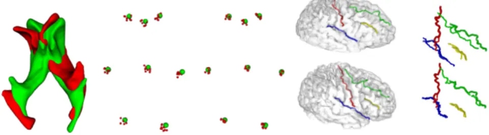
Fig. 3. Experiments on real data. Ventricles: From left to right : X (green) and A(Y ) (red) before registration, position of the 8 anatomical landmarks of the 10 random experiments after registration without priors/constraints and with priors/constraints. Brain: From left to right and top to bottom: 1) brain 1 (top) and brain 2 (bottom); 2) brain 2 (with sulci shown in transparency) towards brain 1 without (top) and with (bottom) using priors/constraints. The four sulci are the central (red), lateral (blue), superior frontal (green) and inferior frontal (yellow) sulci.

3. Marriott, F.H.C.: Separating Mixtures of Normal Distributions. Biometrics 31(3) (1975) 767–769

4. Scott, A.J., Symons, M.J.: Clustering Methods Based on Likelihood Ratio Criteria. Biometrics 27(2) (1971) 387–397

5. Celeux, G., Govaert, G.: A Classification EM Algorithm for Clustering and Two Stochastic Versions. Computational Statistics and Data Analysis 14(3) (1992) 315–332

6. Besl, P., McKay, N.: A Method for Registration of 3-D Shapes. IEEE PAMI 14(2) (December 1992) 239–256

7. Day, N.E.: Estimating the Components of a Mixture of Normal Distributions. Biometrika 56(3) (1969) 463–474

8. Dempster, A.P., Laird, N.M., Rubin D.B.: Maximum Likelihood from Incomplete Data via the EM Algorithm. Journal of the Royal Statistical Society. Series B (Methodological) 39(1) (1977) 1–38

9. Granger, S., Pennec, X.: Multi-Scale EM-ICP: A Fast and Robust Approach for Surface Registration. ECCV (2002) 418–432

10. Chui, H., Rangarajan, A.: A Feature Registration Framework Using Mixture Mod-els. IEEE MMBIA (2000) 190–197

11. Green, P.J.: On Use of the EM for Penalized Likelihood Estimation. Journal of the Royal Statistical Society. Series B (Methodological) 52(3) (1990) 443–452 12. Comb`es, B., Prima, S.: New Algorithms to Map Asymmetries of 3D Surfaces.

MICCAI (2008) 17–25

13. Koenderink, J.J., van Doorn, A.J.: Surface Shape and Curvature Scales. Image and Vision Computing 10(8) (October 1992) 557–564

14. Aouada, D., Feng, S., Krim, H.: Statistical Analysis of the Global Geodesic Func-tion for 3D Object ClassificaFunc-tion. IEEE ICASSP (2007) I–645–I–648

15. Subsol, G., Thirion, J.-P., Ayache, N.: A General Scheme for Automatically Build-ing 3D Morphometric Anatomical Atlases: application to a Skull Atlas. MIA 2 (1998) 37–60

16. Yeo, B.T.T., Sabuncu, M.R., Vercauteren, T., Ayache, N., Fischl, B., Golland, P.: Spherical Demons: Fast Surface Registration. MICCAI (2008) 745–753

17. Durrleman, S., Pennec, X., Trouv´e, A., Ayache, N.: Sparse Approximation of Currents for Statistics on Curves and Surfaces. MICCAI (2008) 390–398