Publisher’s version / Version de l'éditeur:
Vous avez des questions? Nous pouvons vous aider. Pour communiquer directement avec un auteur, consultez la
première page de la revue dans laquelle son article a été publié afin de trouver ses coordonnées. Si vous n’arrivez
Questions? Contact the NRC Publications Archive team at
PublicationsArchive-ArchivesPublications@nrc-cnrc.gc.ca. If you wish to email the authors directly, please see the first page of the publication for their contact information.
https://publications-cnrc.canada.ca/fra/droits
L’accès à ce site Web et l’utilisation de son contenu sont assujettis aux conditions présentées dans le site LISEZ CES CONDITIONS ATTENTIVEMENT AVANT D’UTILISER CE SITE WEB.
5th AIAA Atmospheric and Space Environments Conference, 2013
READ THESE TERMS AND CONDITIONS CAREFULLY BEFORE USING THIS WEBSITE. https://nrc-publications.canada.ca/eng/copyright
NRC Publications Archive Record / Notice des Archives des publications du CNRC :
https://nrc-publications.canada.ca/eng/view/object/?id=e5f505f9-21a9-4af6-b530-83363abad861 https://publications-cnrc.canada.ca/fra/voir/objet/?id=e5f505f9-21a9-4af6-b530-83363abad861
NRC Publications Archive
Archives des publications du CNRC
This publication could be one of several versions: author’s original, accepted manuscript or the publisher’s version. / La version de cette publication peut être l’une des suivantes : la version prépublication de l’auteur, la version acceptée du manuscrit ou la version de l’éditeur.
For the publisher’s version, please access the DOI link below./ Pour consulter la version de l’éditeur, utilisez le lien DOI ci-dessous.
https://doi.org/10.2514/6.2013-2677
Access and use of this website and the material on it are subject to the Terms and Conditions set forth at
Altitude scaling of ice crystal accretion
Altitude Scaling of Ice Crystal Accretion
Tom C. Currie1, Dan Fuleki2, Daniel C. Knezevici3, and James D. MacLeod4 National Research Council of Canada, Ottawa, Ontario, K1A 0R6, Canada
This paper describes experiments performed in an altitude chamber at the National Research Council of Canada (NRC) as the first step towards developing altitude scaling laws and procedures that will possibly allow aero-engines to be certified for operation in ice crystal clouds at high altitude by testing in sea level facilities. The principal objective was to test the hypothesis that accretion within a compressor due to ice crystal ingestion occurs when the local ratio of freestream liquid water content (LWC) to total water content (TWC) lies within a critical range at an accretion-susceptible location. If this hypothesis is correct, the local LWC/TWC ratio is the key parameter that must be matched in tests at low and high pressures to match accretions. Experiments were conducted in a small wind tunnel with an axisymmetric test article, consisting of a hemispherical nose attached to a conical afterbody, at a fixed TWC over a range of LWC/TWC ratios at (absolute) pressures of 34.5 kPa and 69 kPa to test the hypothesis. The LWC/TWC ratio was varied by changing the wet bulb temperature. Accretion steady-state volumes and growth rates measured at the two pressures were compared at conditions which were analytically predicted to produce matched LWC/TWC ratios. Good agreement was achieved in all cases. Accretion growth was greatest for LWC/TWC ratios in the range 10-25%. Additional tests demonstrated that wet bulb temperature, which was identified as an important variable in earlier studies, had little influence on accretion growth beyond its effect on LWC/TWC (i.e. ice particle melting). Tests were also conducted to determine whether accretion growth scales linearly with TWC at constant LWC/TWC. Those tests confirmed that not only does the accretion growth rate in the early growth phase scale in direct proportion to TWC , but so does the final size of the accretion. A simple semi-empirical model for predicting this behavior is described. While most of the tests were conducted with an ice particle median volumetric diameter of 45μ, some of the scaling tests were repeated with larger particles, which produced smaller accretions.
Nomenclature
Copyright © 2013 by Her Majesty the Queen in Right of Canada.
Published by the American Institute of Aeronautics and Astronautics, with permission. 1
&
a, b = TWC-dependent coefficients in relation for t
A = surface area
Cp = specific heat of air at constant pressure
Cice = specific heat of ice
d = diameter
hc = heat transfer coefficient
Levap = latent heat of vaporization of water
Lf = latent heat of fusion of water
Lsubl = latent heat of sublimation of ice
IWC = Ice Water Content (g/m3) LWC = Liquid Water Content (g/m3)
m = mass
= mass flow rate
1
Principal Research Officer, 1200 Montreal Rd., Gas Turbine Laboratory, Building M7, AIAA Senior Member
2
Project Manager, 1200 Montreal Rd., Gas Turbine Laboratory, Building M7, AIAA Senior Member
3
Research Officer, 1200 Montreal Rd., Gas Turbine Laboratory, Building M7, AIAA Member
4
Research Council Officer, 1200 Montreal Rd., Gas Turbine Laboratory, Building M7, AIAA Senior Member
Downloaded by NATIONAL RESEARCH COUNCIL CANADA on June 4, 2020 | http://arc.aiaa.org | DOI: 10.2514/6.2013-2677
5th AIAA Atmospheric and Space Environments Conference June 24-27, 2013, San Diego, CA
10.2514/6.2013-2677 Fluid Dynamics and Co-located Conferences
= mass flux (mass flow rate per unit area)
M = Mach number
MVD = median volume diameter of ice particles, micrometer NRC = National Research Council of Canada
Nu = Nusselt number (= hcd/k)
p = pressure
pref = reference pressure (105 Pa)
Pa = Pascal (N/m2)
Pr = Prandtl number (= µCp/k)
= heat flux
r = radius
RATFac = Research Altitude Test Facility Re = Reynolds number (= ρUd/µ)
t = accretion thickness
to = accretion thickness at stagnation point
t& = thickness growth rate Δttransit = particle transit time
T = temperature
TWC = Total Water Content (= IWC + LWC) Tu = turbulence intensity
U = velocity V, Vol = volume
x = distance (length)
α = ratio of collection efficiency β to ballistic collection efficiency βbal
= collection efficiency
= angle between surface tangent and streamwise direction
δ = increment
stick = sticking efficiency
θ = net melt potential (= Ф – evaporation term)
µ = dynamic viscosity or micron (μm), use should be obvious from context
= kinematic viscosity
= steady-state accretion cone half-angle
ρ = density
ρacc = accretion density (≈( IWC* ρice + LWC* ρliquid)/TWC, for ice and liquid densities ρice andρliquid )
φ = melt potential
= specific humidity (mass of water vapor/unit mass dry air)
Subscripts al = align bal = ballistic cl = centerline conv = convective evap = evaporative g = gas
high, low = high, low pressure
i = injected with the ice grinder or water spray nozzles. Ice or water mass flowrate divided by tunnel air volumetric flowrate to obtain injected quantity
impinge = impingement
l = liquid (water)
m = measured (with SEA WCM-2000 multi-element ice-water content probe)
o = stagnation
p = particle
pc = pressure compensated
2
prof = profile
s = surface
ss = steady-state
sph = sphere
tip = tip of ice growth ts = test section
wb,wbo = wet bulb based on and static or total temperature and pressure ∞ = freestream
I. Introduction
ince 1990, many jet-engine power loss events have been observed at altitudes above 7000m, usually considered to be the upper altitude limit at which water droplets can exist as liquid. These events, which have typically occurred in the anvil region of deep convective systems at tropical latitudes, have included engine rollback, flameout, stall, as well as damage to downstream compressor components from shed ice. As discussed by Mason et al.1 in a comprehensive review of 46 power-loss incidents observed since 1990, it is now generally believed that such events result from atmospheric ice crystals entering the engine core, partially melting, and then refreezing or sticking to internal components.
S
Although many events involving engine performance degradation or damage due to ice crystals have been documented, the comprehension of the phenomenon that would be required either to simulate or replicate it in sea level certification tests is still lacking. Some insight has been gained in the past 6 years in a series of tests performed in the Research Altitude Test Facility (RATFac) at the National Research Council of Canada (NRC), which allows testing with ice particles produced by grinding at chamber pressures down to 20 kPa2. The first of those tests, performed jointly by Boeing, NRC and NASA (National Aeronautics and Space Administration) Glenn Research Center3, used a geometry representative of the S-shaped transition duct between the low pressure and high pressure compressors in a typical jet engine, with an airfoil-shaped strut connecting the inner and outer walls. Accretions were observed on the strut and/or endwall at total air temperatures above and below freezing with ice particles added to the duct airflow, provided (injected) water was also present. The S-duct tests were followed by tests of a wedge-shaped airfoil conducted jointly by NRC and NASA Glenn Research Center4,5. Those tests were the first to demonstrate that a wet bulb temperature (Twb) below freezing is required to obtain strongly adhered hard accretions,
and highlighted the use of Twb instead of dry bulb (static or total) temperature to distinguish between freezing and
non-freezing conditions (due to heat exchange with the environment) for water surfaces exposed to air*.
A test article simulating the outer casing of a compressor with a bleed slot that is typically used to bleed off air before the high pressure compressor has also been tested in RATFac6,8. Those tests demonstrated that accretion growth rate was sensitive to particle size distribution and decreased with increasing particle size, probably due to erosion.
The tests described above provided some insight into the physics of ice crystal icing, but did not attempt to identify scaling parameters that could be matched between low and high pressures/altitudes to match the corresponding ice growth rates or steady-state accretion volumes. Such parameters will be required to allow large aero-engines to be certified for operation in ice crystal clouds at high altitude by testing in sea level facilities, if indeed such certification is even possible. Wet bulb temperature collapses air dry bulb temperature, humidity and pressure into a single parameter separating freezing from non-freezing conditions, as noted above, but its importance beyond that is not clear because significant accretions can be obtained at wet bulb temperatures both above and below freezing4,5,6.
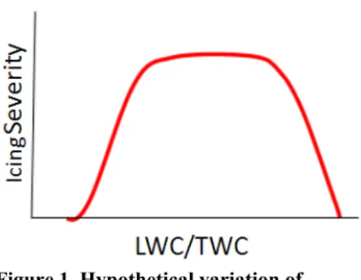
Figure 1. Hypothetical variation of icing severity with LWC/TWC
3
*
Wet-bulb temperature is the temperature of a wet adiabatic surface in an airflow, and is a function of the air dry-bulb temperature, pressure, and moisture content. At a fixed total air temperature (To) and specific humidity (ω), wet
bulb temperature decreases with pressure due to enhanced evaporative cooling.
4
Previous research4,5,6 and a limited amount of engine operational data reported by Mason1 has shown that liquid water is required for ice crystals to accrete on surfaces. It has been theorized, in fact, that an optimum icing regime exists which is a function of the ratio of freestream liquid water content (LWC) to total water content (TWC, sum of LWC and ice water content IWC)1,3, as depicted in Fig. 1. Under glaciated (i.e. fully frozen) conditions, ice particles simply bounce off surfaces, whereas ice particles do not stick and are washed off the surface when too much water is present. In between these extremes, ice buildup is possible, as verified by experiment4,5. The degree to which an icing severity curve such as that shown in Fig. 1 might vary with pressure is unknown, as is the importance of other (non-dimensional) scaling parameters, such as those commonly used to scale cloud icing with supercooled liquid droplets7.
A. Simulation of High Altitude Ice Crystal Icing in Sea Level Facilities
The parameters that can be varied in a sea level aero-engine icing facility to simulate ice crystal events at altitude are quite limited, possibly including only the following:
1) Inlet temperature
2) Ice particle size and concentration
3) Low pressure compressor operating parameters
It is theorized in the present work that the local melt ratio (LWC/TWC) is a key parameter governing ice crystal accretion, so matching ice crystal buildup at some accretion-susceptible location (static components such as stator and guide vanes, casing walls, bleed valves, etc.) in the LP compressor at altitude in a sea level test will require matching LWC/TWC at the same location. This in turn will require matching the total energy transfer to the ice particles between the engine inlet and that location, where such transfer results from energy exchange between particles and air warmed by compression, or from particles impacting surfaces at temperatures above freezing. Because evaporative cooling of the melting ice particles will be more significant at altitude than at sea level, it will likely be necessary to reduce the inlet total temperature in the sea level tests to compensate and obtain the same net energy transfer and resultant melting.
To obtain the same melt profile in the LP compressor at sea level as at altitude, it will likely be necessary to operate the LP compressor at a similar non-dimensional operating point as that of concern at altitude since this will produce similar stage temperature and pressure ratios, and similar Mach numbers and thereby particle transit times. As already noted, a possible test strategy would be to reduce the inlet temperature (if possible) to obtain the same LWC/TWC at a selected (accretion-susceptible) location. A first step in validating such a strategy, however, is to verify that matching LWC/TWC at different pressures produces similar accretions on geometries that are susceptible to accretion. Such geometries are assumed to be those where the Mach number and hence aerodynamic shear stress are low and particles impact the surface at angles close to normal, maximizing collection efficiency. At these angles, reduced mass loss due to particle/droplet bounce and (possibly) erosion would be expected. This study reports the results of such validation experiments, and additional experiments performed to isolate the effects of Twb and TWC.
A simple semi-empirical model of ice crystal accretion is developed to better understand the latter.
II. Test Facility and Test Article
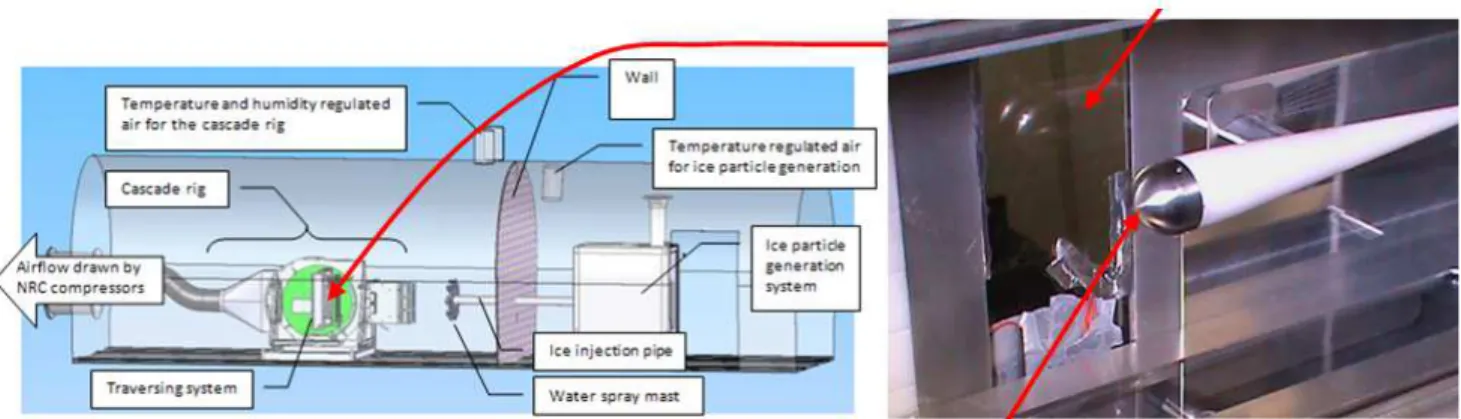
The tests were conducted in a cascade icing tunnel located in the NRC RATFac altitude chamber (Fig. 2). The chamber is divided into hot and cold sides by a partition2. An ice grinder and injection duct are located in the cold side, while the hot side contains the icing tunnel. A flow of cold (~-15°C) dry (-50°C dew point) air with entrained ice particles from the injection duct is mixed with warmer air entering the icing tunnel from the altitude chamber to obtain a required total temperature To at the test section. The relative humidity (RH) of the mixed airflow can be
controlled by varying the humidity of the altitude chamber (warm) air with a humidification system. For a given total pressure po, varying To and RH controls Twb, which in turn controls the degree of natural melting of the ice
crystals. Supplemental water can be injected from a spray mast to raise LWC, if required. The grinder can be configured to deliver different size particles.
Since the principal objective of the scaling tests was to determine conditions and procedures whereby accretions could be matched at low and high pressure, in-situ measurement of ice shape and growth rate was considered a key requirement. Such measurement had proven difficult in previous test programs using two-dimensional airfoil shapes spanning the entire test section due to obscuration of the region of interest at mid span by ice buildup at the airfoil
root and tip4,5. Measurement with laser scanners without first coating the ice with an opaque material (e.g. powder) is also difficult because the translucency of ice produces sub-surface scattering of the laser beam and a resultant error in the measured surface location9. These factors led to the selection of an axisymmetric test article and a photogrammetric method for measuring the ice shape. The test article was a hollow 44.5mm diameter hemispherical nose attached to a streamlined axisymmetric afterbody, shown installed in the 13.2cm x 25.4cm tunnel working section in Fig. 3. The axial centerline of the nose was located on the tunnel centerline. The wall thickness of the nose was 3.175mm. It was fabricated from Ti6Al-4V alloy, due to the widespread use of this alloy in engine compressors, while the afterbody was rapid-prototyped plastic. The nose was wet polished to a surface roughness of ~0.5μ RMS. It was attached to a stepper motor housed in the afterbody, which permitted rotation through 360°. Thirty-six silhouette images of the accreted ice shape were recorded during the 360° rotation for subsequent analysis with commercial 3D photo-modelling software to obtain the 3D ice shape.
Figure 3 also shows the front and rear viewing windows through which the icing tests were recorded with video cameras. Transparent electrical heaters were attached to the windows to mitigate excessive ice buildup.
Figure 2. Icing cascade tunnel installed in NRC RATFac Figure 3. Test article in cascade tunnel, viewed through front window
III. Ice Shape Measurement and Instrumentation
A. Ice Shape Measurement
5
Figure 4. Hemispherical nose replaced by camera calibration disc
The ice shape was measured with commercial 3D photo-modelling
software, 3DSOM. Calibration of the software was performed by providing it with 36 images of its calibration pattern, shown in Fig. 4, recorded during one revolution. Video sequences of the ice shape were then recorded without changing the camera position or field-of-view. The number of video images used to calculate the ice shape matched the number of calibration images (i.e. 36). The 360° rotation of the nose during which the 36 images were recorded was completed in a 2s time period and was repeated every 17s.
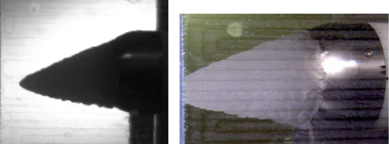
Backlit silhouette and perspective images of a typical ice shape (from run 1197) are shown in Fig. 5. The silhouette images were imported into 3DSOM to calculate the ice shape using the software’s shape-from-silhouette algorithm. The ice shape was then exported as a stereo-lithography (STL) file from 3DSOM and imported into Solidworks CAD software. The volume of the bare nose was subtracted from the volume of the 3D model of the nose and accreted ice to obtain the volume of the
latter. The Boolean subtraction was performed with Solidworks using a 3D solid model of the bare nose. To obtain an exact result with this procedure, the position of a reference point on the bare nose must be exactly matched to the position of the same point on the 3D model with accreted ice. Since it was typically difficult to align these points exactly in the axial (x) direction, the uncertainty in the axial alignment δx produced a corresponding uncertainty in the net ice volume, designated δVal. The value of δx was estimated to be ~ (±)0.75mm, from which δVal was
estimated by performing the Boolean subtraction twice with the bare and iced models offset axially first by + δx and then by –δx from the nominal alignment. The value of δVal was then assumed to be one-half of the difference
between the resulting net ice volumes.
The uncertainty in the ice volume contained an additional component δVprof resulting from uncertainties in the
location of the accretion profile, which was typically approximately conical in shape. The edge of the ice was seen as a gradient in pixel intensity in the images processed with 3DSOM, where the pixels would transition from light to dark over a distance of approximately 3 pixel widths. The uncertainty in the surface location was assumed to be ±1 ½ pixels, or ~0.33mm for the pixel width of ~ 0.22mm used in the images. This uncertainty was multiplied by the area of the ice surface to convert it to a volume.
Figure 6a shows a photo-realistic colored (3D) model of the run 1197 ice shape obtained with 3DSOM, while Fig. 6b shows an STL model of the net ice shape obtained by subtracting the bare nose. Although, the tip of the accretion is rounded slightly and the finer details of the ice shape are lost in the 3D model, these deficiencies are not expected to affect the computed volume of the accretion significantly.
Figure 5. Backlit silhouette and perspective images of final ice shape in run 1197
Figure 6a. Photo-realistic 3D model of run 1197 Figure 6b. STL model of net ice shape for run 1197 accretion from 3DSOM
6
7
Only steady-state ice shapes were processed with 3DSOM. To allow comparison of ice shapes produced at low and high pressures during the growth phase of each icing run, commercial video analysis software (ProAnalyst Lite v1.5.5.8) was used to extract 2D profiles of the ice shape from the silhouette images. This process did not use video images recorded during the 360° rotations performed every 17s but rather extracted the ice profiles from the backlit images recorded midway between the rotations. With each such image, points were inserted manually along the edge of the ice shape, typically at ~14 locations, and then joined by line segments to obtain the 2D profile.
B. Instrumentation
A traversable 3-hole cobra-style probe with integrated To sensor was used to measure po, To, and velocity under
dry conditions (i.e. without ice and/or water injection). As in previous tests, a WCM-2000 multi-element probe, developed by Science Engineering Associates Inc.(SEA), was used to obtain measured values of liquid water content (LWC) and total water content (TWC), designated LWCm and TWCm respectively. A traversable
NRC-proprietary “TAT-RH” probe was used to measure To and humidity with mixed-phase flow present (i.e. under “wet”
conditions). These “wet” values of To and humidity were used with the value of po measured with the 3-hole probe
to calculate Twbo under wet conditions. Humidity measurements obtained with this probe under dry tunnel conditions
were also used with po and To to calculate the dry Twbo before each test point. Unless otherwise noted, quoted values
of all parameters apply at the tunnel centerline on a measurement plane ~150mm upstream of the test article.
The measurement accuracies of the different test parameters are given in Ref. 2: the uncertainties in LWCm and
TWCm are not provided because they are unknown at the present time. IV. Test Conditions and Procedure
All of the tests were performed at a Mach number (M) of 0.25. Tests were carried out at two total pressures: 34.5kPa (5 psia) and 69kPa (10 psia). The wet bulb temperature was varied from -2°C to 6°C at each pressure, which required using a lower total air temperature at 69kPa than at 34.5kPa to compensate for the reduced evaporative cooling. The total air temperature was nominally 15°C and 8°C for all of the tests at 34.5kPa and 69kPa respectively, resulting in corresponding static temperatures of ~11.5°C and 4.5°C.
Two grinder configurations were used, designated A and B for configurations which produced the smallest and larger particles respectively. The median volume diameter (MVD) of the smaller particles, measured with a shadow imaging technique, was ~45μ, while size data for the larger particles are not yet available. Other size statistics for the small particles and a description of the measurement technique are given by Knezevici et al8. The median volume diameter (MVD) of the water droplets for the spray used, when required to supplement the water produced by natural melt of the ice particles, was 40µ based on sea level calibration data and unadjusted for evaporation.
The SEA multi-wire probe is believed to produce erroneous results for TWC in particular2, where errors in TWC occur because the trough used to measure TWC fails to retain all of the impinging ice particles. In a test sequence at given values of M, To, po and particle size, the strategy used to set TWC was to increase LWC/TWC at a fixed
injected ice water content IWCi (bulk ice mass flowrate/tunnel volumetric flowrate) by increasing the humidity and
therefore Twbo. It is assumed the centerline TWC, designated TWCcl, did not change from its initial value in this case
because the ice flow was not changed. TWCcl was calculated from IWCi under glaciated conditions as described in
Ref. 2 and was within 5% of IWCi in all cases. All values of TWCcl were within 9% of 8g/m3 , except for two runs
performed to assess the dependence of accretion growth on TWC for otherwise fixed conditions. The full test procedure was as follows:
1) The grinder was configured to give the required particle size.
2) The tunnel operating point was adjusted to obtain the required M, To and po.
3) The humidity was set to a low value to obtain glaciated conditions (Twbo < 0°C)
4) The bulk ice flow was set to give IWCi ~ 8g/m3. At each new particle size, the SEA probe was traversed to
obtain a concentration factor C, discussed in Ref. 2, from which TWCcl = C*IWCi. As mentioned above, all
values of TWCcl calculated in this manner were within 9% of 8g/m3.
5) In a typical test sequence, the bulk ice flow was held fixed and the humidity was increased in steps to increase Twbo and thereby the melt ratio.
6) The following steps were followed at each test condition:
a) The centerline values of po and To were measured with the 3-hole probe before each test, followed by
measurements of centerline To and specific humidity ∞ with the TAT-RH probe.
b) The ice flow and video cameras were started, along with the stepper motor controller which rotated the hemispherical nose of the test article every 17s.
c) The ice flow was turned off for ~30s after the accretion stopped growing to obtain clear video images of the ice shape.
d) The ice flow was restarted and LWCm, TWCm were measured at the centerline with the SEA probe.
e) The centerline values of To and ∞ were measured with the TAT-RH probe.
f) The ice flow was turned off and the test article allowed to de-ice.
V. Data Reduction
In order to match values of LWC/TWC at potential accretion sites in the LP compressor of an engine operating at altitude in a sea level test by specifying appropriate changes to the inlet conditions, particularly inlet temperature, it will be necessary to correctly scale the melting of ice crystals in the compressor with altitude. In the case of the RATFac tests, the most relevant scaling procedure would therefore be one in which ice shapes were matched at low and high pressures by matching a melting scaling parameter derived from tunnel conditions po, To and ∞, instead of
matching measurements of melt ratio (i.e. either LWCm/TWCm or LWCm/TWCcl ) at the test section. In addition to
being more easily applied to engine tests, such a procedure would not be influenced by errors in melt ratio measurement with the multi-wire probe, errors which are not well understood.
Theoretical expressions relating melt ratio to ∞ and tunnel static conditions T∞ and p∞ are derived in Appendix A, where the following relation is obtained for LWC at the test article (Eq. A.29):
f transit ts total cA t L h LWC≈ θ Δ / (1)
where hc is the particle heat transfer coefficient, Atotal is the total surface area of the particles/unit volume of air, Lf is
the latent heat of fusion of water, Δttransit is the particle transit time in the tunnel, and ts is the (net) melt potential at
the test section, defined by
) 611 ( 1974 ~ , ∞ ∞ ∞ − − p p T l ts θ for ∞ ∞ ∞ ∞ = +ω ω 622 . 0 , p pl (2)
where pl,∞ is the vapor pressure of water in the freestream. Temperatures are in °C and pressures are in Pa in Eq. 2,
which was evaluated using “wet” values of T∞ and ∞ (i.e. values obtained with ice flow using the TAT-RH probe).
The measure of melt ratio to be used for scaling is LWC/TWCcl, where LWC is calculated from Eq.1 by substituting
the tunnel test conditions (T∞, p∞, ∞) into Eq.2. Ice accretions observed at pressures p∞,low and p∞,high will be
compared for tests with the same particle size under conditions where
low cl high cl p TWC LWC p TWC LWC , , @ @ ∞ ≈ ∞ (3)
Although the expressions for LWC at p∞,low and p∞,high contain the terms Atotal, Δttransit and hc, it is assumed that
Atotal is proportional to TWCcl, for a fixed particle size, and therefore remained approximately constant when particle
size was held constant. Likewise, it is assumed that Δttransit is proportional to 1/M and therefore did not change
significantly in the tests, which were all performed at M=0.25. With these simplifications, the matching condition defined by Eq. 3 becomes
low ts c high ts c p h p hθ @ ∞, = θ @ ∞, (4)
Preliminary attempts to match ice shapes for conditions satisfying Eq. 4 assuming hc did not depend on pressure
produced unsatisfactory results, so hc was assumed to be related to pressure through a power law obtained by
retaining only the second (Rep dependent) term in Eq. A.5. Assuming the particle-to-gas relative velocity Up,rel used
in the particle Reynolds number Rep is not a strong function of pressure*, the following relation defines the ratio of hc values at low and high pressures
8
*
This will be the case if Rep is low enough for the Stokes term in the particle drag law to predominate.
n high low high c low c p p p h p h ⎟ ⎟ ⎠ ⎞ ⎜ ⎜ ⎝ ⎛ = ∞ ∞ ∞ ∞ , , , , @ @ (5)
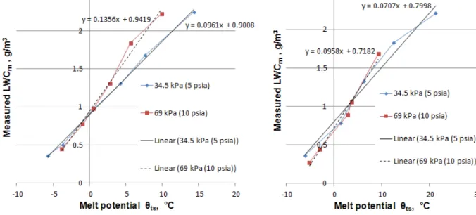
If Eq. 1 correctly describes the dependence of LWC on ts, LWC should vary linearly with ts and Atotalhc should
be proportional to the slope (∂LWC/∂ ts) of a linear fit to the data. Figures 7 and 8 plot LWC against ts for the
small and large particles respectively using the multi-wire measurements for LWC (i.e. LWCm). Since the curves are
close to linear, as expected, linear regressions were performed to obtain the curve fits shown on the figures for LWCm vs. ts. The slopes were used in Eq.5, rewritten as
n high low high ts m low ts m low total high total p p p LWC p LWC p A p A ⎟ ⎟ ⎠ ⎞ ⎜ ⎜ ⎝ ⎛ = ∂ ∂ ∂ ∂ ∞ ∞ ∞ ∞ ∞ ∞ , , , , , , @ / @ / @ @ θ θ (6)
to evaluate the exponent n. Equation 6 was evaluated assuming Atotal for each particle size and pressure combination
was proportional to the corresponding value of TWCcl. The resulting values of n for the small and large particles
were 0.32 and 0.44 respectively. The average of these values, 0.38, was then used to define a pressure-compensated net melt potential, θpc, where
pc = ts (p∞/pref)0.38 (7)
with pref =100 kPa. The exponent of 0.38 is close to the Reynolds number exponent of 0.5 recommended by Ranz
and Marshall12, used in Eq. A.5, suggesting the particle Reynolds numbers were high enough for the laminar (Stokes) term in Eq. A.5 to be relatively insignificant.
Figure 7. LWCm vs. θts for small particles Figure 8. LWCm vs. θts for large particles
VI. Results
A. Grinder Configuration A (Small Particles)
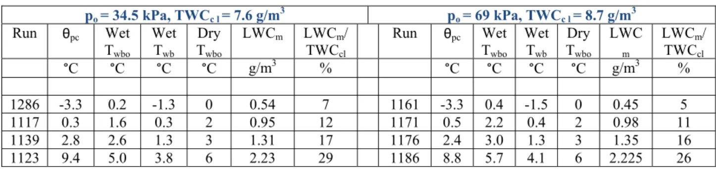
Values of θpc were matched as closely as possible in runs at 34.5kPa and 69kPa to obtain the pairings listed in
Table 1. Each row lists the paired runs for the two pressures. The pairs are listed in order of increasing θpc and
therefore melt ratio. Except for the pair of runs at the highest Twbo, where the θpc values for the two pressures differ
by 0.6°C, the θpc values for all of the remaining pairs agree within 0.3°C. Likewise, the values of LWCm and
LWCm/TWCcl for each pair are in good agreement.
9
Table 1 also lists values of dry and wet Twbo and wet Twb (i.e. wet bulb temperature based on static conditions,
which should correlate better with ice particle melting than Twbo). It is apparent that all of the wet bulb temperatures
are well matched in the paired runs, so it would have made little of no difference if the pairing had been based on (any) wet bulb temperature instead of θpc. The parameters θpc and wet Twb are actually related, as discussed in
Appendix A where the following equation is derived(Eq. A.18)
Table 1. Runs with grinder configuration A at 34.5 kPa and 69 kPa with closely matched θpc
po = 34.5 kPa, TWCc l = 7.6 g/m3 po = 69 kPa, TWCc l = 8.7 g/m3 Run θpc Wet Twbo Wet Twb Dry Twbo LWCm LWCm/ TWCcl Run θpc Wet Twbo Wet Twb Dry Twbo LWC m LWCm/ TWCcl °C °C °C °C g/m3 % °C °C °C °C g/m3 % 1286 -3.3 0.2 -1.3 0 0.54 7 1161 -3.3 0.4 -1.5 0 0.45 5 1117 0.3 1.6 0.3 2 0.95 12 1171 0.5 2.2 0.4 2 0.98 11 1139 2.8 2.6 1.3 3 1.31 17 1176 2.4 3.0 1.3 3 1.35 16 1123 9.4 5.0 3.8 6 2.23 29 1186 8.8 5.7 4.1 6 2.225 26 ∞ ∞ − − + = T p p Twb 1741([ lTwb 611])} 0.134 { 134 . 1 ,
θ
(8)where pl,Twb and 611 are the vapor pressures of water (in Pa) at temperatures of Twb and 0°C respectively. Since the
values of Twb of interest are close to 0°C, the term in square brackets can be linearized using the derivative of the
vapor pressure of water with respect to water temperature at values near freezing. This derivative increases from ~ 45 Pa/°C at 0°C to ~57 Pa/°C at the highest wet Twb of ~4°C seen in Table 1, and has an average value of ~ 50 Pa/°C
between 0°C and 4°C. Using the latter value, the term in square brackets can be replaced by 50Twb. The value of T∞
was ~ 11.5°C and 4.5°C in all of the tests at 34.5kPa and 69kPa respectively, so 0.134 T∞ is ~1.5°C at 34.5kPa and
0.6°C at 69kPa. It is also easily verified using the Twb values in Table 1 and the high and low values of p∞ (~66 kPa
and 33 kPa) that the second term involving T∞ is small compared to the first, at least for the highest Twb tests. If this
term is ignored for simplicity, the ratio of Twb at high pressure to Twb at low pressure can be written as
] ) / 87050 ( 1 ) / 87050 ( 1 ) / ( [ , , , , , , , , high low n high low low pc high pc low wb high wb p p p p T T ∞ ∞ ∞ ∞ + + = θ θ (9)
where n is the pressure exponent introduced in Eq. 6 and assigned a value of 0.38. The term in square brackets in Eq. 9 has a constant value of ~1.2 for all of the pairs of scaling tests, allowing Eq. 9 to be rewritten as
) 2 . 1 1 ( , , , , , low pc high pc low wb high wb low wb T T T θ θ − = − (10)
≈−0.2Twb,low (for θpc,high/ θpc,low ≈1) (11)
Equation 11 shows that the difference between wet Twb values at high and low pressures will be small when Twb is
itself small, as in the scaling tests. Eq. 9 shows that the similarity of high and low pressure wet Twb values seen in
Table 1 at approximately matched θpc (i.e. θpc,high/ θpc,low ≈1) would not apply universally, since it depends on the
independent values of p∞,high, p∞,low and n. That similarity was observed in the present tests because the term in
square brackets in Eq. 9 is close to unity.
It is noteworthy that significant melting (i.e. LWCm > 0.5 g/m3) was obtained at wet Twb < 0°C, as seen in Table
1. Melting can occur in the RATFac facility at test section Twb below freezing because the desired air temperature at
the test section is obtained by mixing cold dry air from the injection jet with warm more humid air from the test cell, as discussed previously. The temperature of the test cell air was typically ~23°C at 34.5 kPa and ~13°C at 69 kPa in the scaling tests. Ice particles at the boundary of the injection jet are exposed to temperatures approaching that of the test cell air as the cold and warm flows mix, potentially producing melting even when the test section Twb is below
10
freezing. Another related factor is that the SEA multi-wire probe typically gives a small LWC reading even when the flow is fully glaciated. The measured value of this offset, determined by measuring LWCm at a dry Twb of -3°C,
was ~ 0.2 g/m3 in the scaling tests at both pressures with IWCi ~ 8g/m3, or 2.5% of TWCcl. This offset has not been
applied to any of the LWCm values given in this paper.
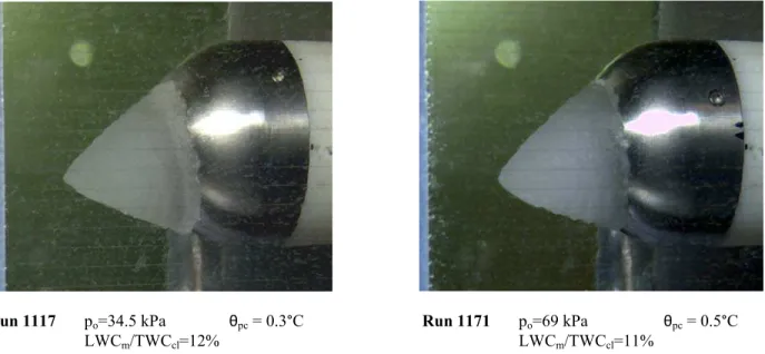
Images of the final (steady-state) ice shapes for each pair of runs are given in Figs. 9-12. The final ice shapes for each pair appear quite similar, and vary from small to large to small again with increasing melt ratio, in agreement with the hypothetical dependence of icing severity on melt ratio shown in Fig. 1. Comparing the size of the accretions in Fig. 9 to those in Fig. 10, it is clear that accretion size is strongly dependent on the melt ratio LWCm/TWCcl, which increases by only 5-6 percentage points from the runs in Fig. 9 to those in Fig. 10.
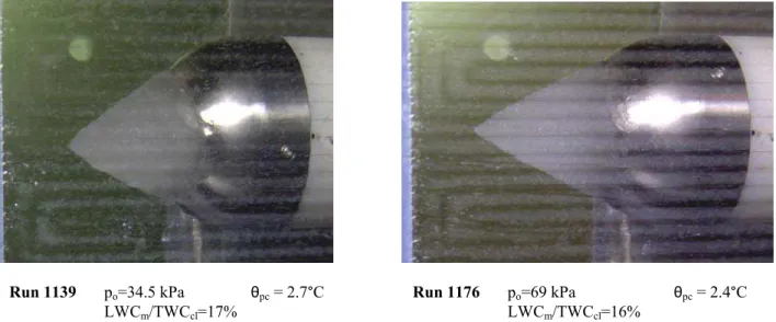
Accretion shapes were typically conical, as seen in Figs. 9-12. Axisymmetric growth ceased if the tip of the accretion started to drop due to gravity forces.
Run 1286 po=34.5 kPa θpc = -3.3°C Run 1161 po=69 kPa θpc = -3.4°C
LWCm/TWCcl=7% LWCm/TWCcl=5%
Figure 9. Comparison of steady-state ice shapes for low and high pressure runs 1286 and 1161 at approximately matched θpc
Run 1117 po=34.5 kPa θpc = 0.3°C Run 1171 po=69 kPa θpc = 0.5°C
LWCm/TWCcl=12% LWCm/TWCcl=11%
Figure 10. Comparison of steady-state ice shapes for low and high pressure runs 1117 and 1171 at approximately matched θpc
11
Run 1139 po=34.5 kPa θpc = 2.7°C Run 1176 po=69 kPa θpc = 2.4°C
LWCm/TWCcl=17% LWCm/TWCcl=16%
Figure 11. Comparison of steady-state ice shapes for low and high pressure runs 1139 and 1176 at approximately matched θpc
Run 1123 po=34.5 kPa θpc = 9.4°C Run 1186 po=69 kPa θpc = 8.8°C
LWCm/TWCcl=29% LWCm/TWCcl=26%
Figure 12. Comparison of steady-state ice shapes for low and high pressure runs 1123 and 1186 at approximately matched θpc
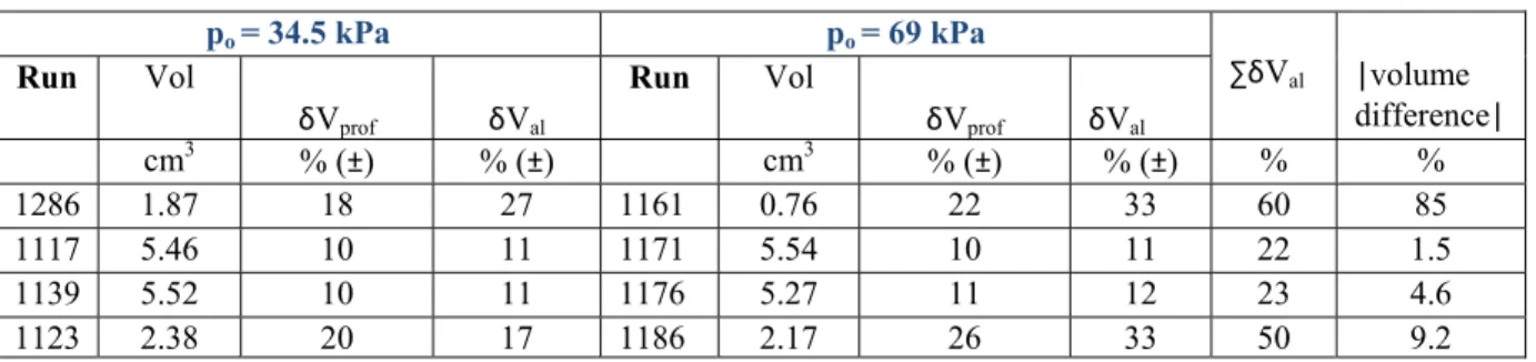
Estimates of the final volume of ice accreted in each run and the corresponding uncertainties are included in Table 2, which shows that δVal was usually larger than δVprof. The volume difference in the last column is normalized by
the average of the high and low pressure volumes. When comparing the difference between ice volumes measured at 34.5kPa and 69kPa to the uncertainty in the measurement to determine whether the difference is statistically significant, δVprof should probably be excluded from the measurement uncertainty because a consistent pixel
intensity threshold (~50%) was used to detect the edge of the ice in all calculations. When only δVal is considered,
the volume differences in the last column of Table 2 are less than the sum of the δVal values for the 34.5 and 69kPa
tests (second to last column) for all pairs of tests except 1286 and 1161. The statistically significant difference for these tests probably resulted from the difference in LWCm/TWCcl, which was only 5% in run 1161 with the smaller
accretion compared to 7% in run 1286.
12
Table 2. Estimates of steady-state ice volumes for runs at matched θpc po = 34.5 kPa po = 69 kPa ∑δVal |volume difference| Run Vol δVprof δVal Run Vol δVprof δVal cm3 % (±) % (±) cm3 % (±) % (±) % % 1286 1.87 18 27 1161 0.76 22 33 60 85 1117 5.46 10 11 1171 5.54 10 11 22 1.5 1139 5.52 10 11 1176 5.27 11 12 23 4.6 1123 2.38 20 17 1186 2.17 26 33 50 9.2
In addition to using final ice volumes to compare accretions at low and high pressures, additional comparisons were performed using accretion shapes recorded during the growth phase and reduced with ProAnalyst, as discussed previously. The resulting profiles for runs 1117 and 1171 are compared in Fig. 13 at three time intervals from the time ice growth was first observed. The agreement is good at 230-233s , when both accretions had stopped growing, as well as during the growth phase at the intermediate time intervals of 33-35s and 117-118s. The good agreement at both time periods in the growth phase indicates the growth rates were closely matched in the two runs.
Figure 13. Ice profiles for runs 1117 and 1171 at 33-35s, 117-118s and steady-state (230-233s)
1. Effect of Wet Bulb Temperature at Fixed Melt Ratio
It has been hypothesized that accretion growth depends principally on the melt ratio LWC/TWC and that the influence of Twbo is largely limited to its effect on this ratio. To confirm this, additional tests were performed in
which Twbo was varied while melt ratio and TWC were held approximately constant. This was done by first selecting
two runs, one with a relatively low (dry) Twbo of 0°C, and therefore little accretion, and another with a higher Twbo (2
or 3°C) and correspondingly more accretion. The low Twbo run was then repeated with supplemental water added via
the spray mast and the ice flow adjusted to match LWCm and TWCm to their values measured in the higher Twbo test.
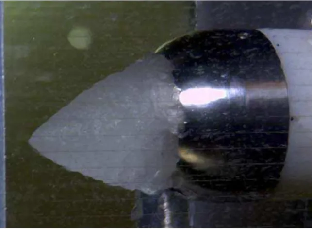
For example, Fig. 9 shows the steady-state accretion for run 1286 (dry Twbo = 0°C) while Fig. 14 shows the accretion
for run 1291 performed at the same pressure (34.5kPa) but with a higher dry Twbo of 3°C. The measured LWCm and
TWCm values in run 1291 were 1.30 g/m3 and 3.08 g/m3 respectively. These values were closely matched in run
1308, which was performed at the lower dry Twbo of 0°C, by adding supplemental water and adjusting the ice flow.
The resulting LWCm and TWCm values were 1.30 g/m3 and 3.02 g/m3 respectively. Figure 15 shows the resulting
accretion for run 1308, which closely matches that shown in Fig. 14 for run 1291 in spite of the reduction in dry Twbo
13
from 3°C to 0°C. It is worth noting that the wet values of Twbo were 2.6°C and 1.0°C in runs 1291 and 1308
respectively, so the reduction was not as great as for the dry Twbo. Nonetheless, Twbo variations within this range had
little effect on accretion size.
Figure 14. Accretion in run 1291 with dry Twbo=3°C Figure 15. Accretion in run 1308 with dry Twbo =0°C and supplemental water added to
match LWCm and TWCm for run 1291 (Figure 14)
The independent effect of Twbo was assessed in a second series of tests at 34.5 kPa. The high Twbo test in this series
was run 1117, shown previously in Fig. 10. The low Twbo test without supplemental water was run 1113 (Fig. 16),
while run 1149 (Fig. 17) was the test in which supplemental water was added and the ice flow was adjusted to match LWCm and TWCm to the values measured in run 1117. The accretions at matched LWCm and TWCm seen in Fig.10
and Fig. 17 are clearly very similar. The wet Twbo was 1.6°C in run 1117 and 0.4°C in run 1149 so the difference
(1.2°C) was slightly less than the corresponding value of 1.6°C for the previous comparison with runs 1291 and 1308. Additional comparisons with larger differences would be beneficial.
Dry Twbo=0°C Wet Twbo=-0.1°C Dry Twbo=0°C Wet Twbo=0.4°C
LWCm=0.36 g/m3 TWCcl=8 g/m3 LWCm=1.07 g/m3 TWCm=2.27 g/m3 Figure 16. Accretion in run 1113 Figure 17. Accretion in run 1149 with
supplemental water added to match LWCm
14
Figure 18 compares ice shapes obtained from processing silhouette images for runs 1117 and 1149 at two time intervals during the growth phase, 33s and 117s from the time ice growth was first observed, as well as at 230-234s
Figure 18. Ice shapes in runs 1117 and 1149 at 84s and 146-150s after the start of ice growth.
when both accretions had stopped growing. The profiles are well-matched at 33s and at steady-state, but the profile for run 1149 appears to be lagging that for run 1117 slightly at 117s. Nonetheless, the growth rates and asymptotic ice volumes were similar in the two runs.
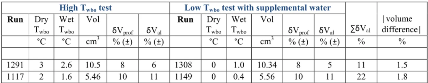
Estimated ice volumes for the two pairs of runs performed to assess the independent effect of Twbo, discussed above, are given in Table 3. The
estimated ice volumes are well matched for the high Twbo run and the corresponding low Twbo run
with supplemental water.
Table 3. Estimates of steady-state ice volumes for Twbo sensitivity tests
High Twbo test Low Twbo test with supplemental water
∑δVal |volume difference| Run Dry Twbo Wet Twbo Vol δVprof δVal Run Dry Twbo Wet Twbo Vol δVprof δVal °C °C cm3 % (±) % (±) °C °C cm3 % (±) % (±) % % 1291 3 2.6 10.5 8 6 1308 0 1.0 10.34 8 5 11 1.5 1117 2 1.6 5.46 10 11 1149 0 0.4 5.56 10 11 22 1.8 2. Effect of TWC
Figure 19. Accretion in run 1202 with TWCcl=4 g/m3
It has been observed in previous studies that ice growth sometimes appears to scale supra-proportionally with TWC5. This is important because high levels of TWC could occur within an aero-engine low pressure compressor due to centrifuging of particles towards the outer casing, scoop factor effects at low engine powers during descent, and changes in flowpath geometry. To investigate this effect further, additional runs with varying TWCcl were
conducted at po = 69 kPa. The dry Twbo was held constant at 3°C, and the injected ice flow was increased, without
adding supplemental water, to obtain TWCcl values of 4 g/m3 (run 1202), 8.7 g/m3 (run 1176) and 17.4 g/m3 (run
1197). Figure 11 shows the steady-state accretion for run 1176, while the steady-state accretions for runs 1202 and 1197 are shown in Figs. 19 and 5 respectively. Accretion growth clearly increased dramatically as TWCcl was
increased. Although the melt ratio LWCm/TWCcl dropped to ~13% in run 1197
from ~16% in runs 1202 and 1176, comparison of the accretions in Figures 10 and 11 indicates the sensitivity to melt ratio is small to non-existent in this range. The differences in accretion growth in the 3 runs are therefore attributed to variations in TWCcl, not melt ratio.
Figure 20 compares ice shapes obtained with ProAnalyst software for runs 1176 and 1197 at an intermediate time of 79s from the start of ice growth and at times close to the end of the runs, when both accretions had stopped growing. Since TWCcl in run 1176 was ½ that in run 1197, the horizontal growth for run
1197 has been scaled by a factor of ½ to normalize the growth rates to the TWCcl used in run 1176 (8.7g/m3 ). A similar comparison for earlier times of
30s and 62s is included in Fig. 21. The growth curves in Figs. 20-21 indicate the normalized growth rate in run 1197 only slightly exceeded that in run 1176.
15
The reasonably good agreement at earlier times shows that growth rate was almost proportional to TWCcl during
the early growth phase, as one would intuitively expect, but the agreement at 160s-179s when growth had stopped indicates the accretion steady-state size also scaled directly with TWCcl. The latter result is surprising because
growth stops when the mixed-phase mass flux impinging on the surface of an accretion equals the mass flux being lost due to melting, evaporation, particle/droplet bounce, erosion of existing ice, runback, splashing of any water film present, etc. Some of the loss mechanisms can be expected to depend on the angle between the surface and the impinging particles, but many of the mass loss fluxes, such as those due to bounce and erosion, might also be expected to scale directly with the impinging mass flux, at least at low values of the latter. Doubling the impinging mass flux by doubling TWCcl would simply double such proportional mass loss fluxes and would not alter the
equilibrium surface angle provided they represented the dominant loss mechanisms. Further research is required to better understand the relative importance of the different loss mechanisms.
Figure 20. Comparison of run 1176 ice profiles at 79s Figure 21. Comparison of run 1176 ice profiles and at steady-state (160s-179s) to scaled profiles for at 30s and 62s to scaled profiles for run 1197 run 1197
The results in Figs. 20 and 21 can be used to estimate the fraction of the impinging mixed-phase mass flux that was lost due to the effects mentioned above. To that end, the ice thickness at the nose of the hemisphere at 30s obtained from Fig. 21 was averaged for runs 1176 and 1197 and divided by the 30s time interval to obtain a thickness growth rate tof ~0.26 mm/s. For the conditions prevailing during these tests and the particle MVD of 45μ, collection efficiency calculations published by Dorsch et al.10 for a sphere in crossflow provide a value of ~0.94 at the forward stagnation point. With this collection efficiency, the maximum theoretical value of the growth rate at the stagnation point can be calculated by assuming all of the mixed-phase particles impacting the surface stick (i.e. do not melt, run back or bounce off the surface) and do not erode the surface. With this assumption, is given by
& max t& max t& acc cl U TWC t&max=0.94 * ∞/
ρ
(12)where U∞ is the freestream velocity and ρacc is the accretion density, assumed for this simplified analysis to be
calculable directly from LWCm and IWCcl using the densities of liquid water and ice respectively. For U∞ = 84m/s
and with ρacc evaluated using the LWCm and IWCcl values for runs 1176 and 1197, Eq. 12 gives t&max≈ 0.73mm/s for
16
TWCcl=8.7g/m3. The measured of 0.26 mm/s is approximately 35% of , indicating that approximately 65% of
the impinging mixed-phase flow was lost due to the mechanisms mentioned previously. Although it is difficult to apportion these mechanisms to the total loss, it is possible to demonstrate that the loss due to melting and evaporation combined (i.e. the ablative loss) is insignificant because it can be estimated from equations given in Appendix A. The melt and evaporation rates per unit surface area due to energy transfer from the air, and respectively, can be estimated from Eqs. A.6 and A.12 (with To and po substituted for T∞ and p∞) by taking Ap
to be a unit area of the accretion surface and using ∞ and To derived from wet measurements with the TAT-RH
probe at the test section measurement plane. The heat transfer coefficient hc needed to evaluate these mass fluxes
can be obtained from the approximate correlation
t& t&max
" melt m " evap m sph sph sph
Tu
Nu
=
1
.
19
Re
+
0
.
02
∞Re
(13)which applies to air and was derived from a graph (approximately linear) of Nusph /√Resph vs. Tu√Resph given in Fig.
4 of Ref. 11. The parameter Nusph (=hcdsph/kg, for gas thermal conductivity kg) in Eq. 13 is the Nusselt number at the
stagnation point on a sphere of diameter dsph, while Resph (=U∞ dsph / g) is the sphere Reynolds number and Tu∞ is
the freestream turbulence intensity. Using a measured Tu∞ of 0.0775 (i.e. 7.75%) for the RATFac icing tunnel at
M=0.252, Eq.13 gives hc≈460 W/m2°C for the conditions in Runs 1176 and 1197. Using To, po and ∞ from these
runs with this hc, the resulting ablative mass fluxes for runs 1176 and 1197 are only 0.0093 kg/m2s and 0.0081
kg/m2s respectively. These mass fluxes would produce corresponding surface recession (i.e. loss) rates ) of 0.01mm/s and 0.009 mm/s for an estimated ρacc = 932 kg/m3 (~16% liquid), which are both
insignificant compared to the total loss of 0.47mm/s. Dissipation of the kinetic energy of the impinging ice particles would have produced additional melting, but it is easily verified that this could not have melted more than 1% of the impinging ice mass flux. These results suggest that the low measured growth rate was produced primarily by mechanisms other than melting and evaporation.
acc evap m" )/
ρ
+ melt m (& ''The results of the preceding order-of-magnitude estimate of the surface recession rate produced by melting and evaporation also explain why Twbo had little independent effect on accretion, because it is believed these are the only
phenomena affected by Twbo apart from the ice particle melt ratio. This observation assumes the wet Twbo is above
freezing, as was the case in the present tests (the wet Twbo was 2.4°C and 3°C in run 1197 and 1176 respectively) and
ice has adhered well enough to the surface for ice growth to start. The wet Twbo can affect the surface temperature,
which in turn would affect adhesion to a bare surface5. As such, Twbo may have a more significant effect on the
initiation of accretion than on the growth of ice-on-ice. 3. First-Order Accretion Model
Although the loss mechanisms responsible for the variations in accretion size seen in runs 1202, 1176 and 1197 are not well understood, those variations can nonetheless be captured with a relatively simple semi-empirical model described in Appendix B. The accretion growth histories for runs 1176 and 1197, in particular, can be predicted with reasonable fidelity using a local growth rate defined by Eq. B.13, as seen in Figs. B.3 and B.4. The angle in Eq. B.13 is the local surface inclination, shown in Fig. B.1. These results suggest that it may be possible to predict ice-to-ice growth rates using correlations or semi-empirical relations for the local sticking efficiency stick , where stick is
defined by Eq. B.14.
B. Grinder Configuration B
Results obtained with the larger particles produced by grinder configuration B were similar to those obtained with
configuration A except accretions were much smaller. This is illustrated in Figs. 22 and 23, which show accretions observed in runs 1428 and 1385 at 34.5kPa and 69kPa respectively and matched values of θpc. The accretions shown
were the largest observed with large particles at any melt ratio. The reduction in accretion size with increasing particle size corroborates the conclusions of Knezevici et al.6,8 regarding the importance of particle size. As with the smaller particles, the size of the accretions grew rapidly as the melt ratio LWCm/TWCcl was increased from 5-11%,
and then dropped when this ratio was raised above 23-25%.
17
Figure 22. Accretion with large particles in run 1428 Figure 23. Accretion with large particles in run 1385 LWCm/TWCcl = 23% θpc=8.2°C LWCm/TWCcl = 22.4% θpc=8.0°C
VII. Conclusions
Both the steady-state size and growth rate of accretions on a test article with a hemispherical nose were duplicated in tests conducted at pressures of 34.5 kPa (5 psia) and 69 kPa (10 psia) when the melt ratio was matched, either by matching the measured liquid water content LWCm (or LWCm/TWCcl) or the pressure-compensated melt potential
θpc. The latter parameter was derived so that the melt ratio is directly proportional to it for a fixed particle size and
transit time. Accretion size was found to be very sensitive to melt ratio, increasing rapidly as LWCm/TWCcl was
raised from~5% to ~11%, and then falling again at higher LWCm/TWCcl in the 23-25% range. The successful use of
melt ratio as the sole parameter for scaling pressure effects indicates that unrelated parameters which also depend on pressure (density), such as particle and droplet collection efficiencies and aerodynamic shear stress, played a relatively minor role for the test article and test conditions used in this study.
Accretion size was not sensitive to wet bulb temperature Twbo at a fixed melt ratio, suggesting that the additional
water produced by melting of the surface deposits by energy exchange with the airflow was small relative to the impinging mass flux of (liquid) water. Order-of-magnitude estimates of this melt rate confirmed this observation. It is noteworthy, however, that while θpc was derived as a pressure scaling parameter for melting ice crystals, it should
also scale the pressure dependence of the melt mass flux (i.e. melt rate per unit surface area) on a mixed-phase surface deposit approximately correctly if the heat transfer coefficient on the deposit scale scales with pressure according to Eq. 5 (i.e. has the same exponent n).
Tests with varying TWC at fixed LWC/TWC showed that accretion growth rate scales proportionally with TWC in the early phases of ice growth, as does the steady-state size of the accretion. Additional research into loss mechanisms (i.e. mechanisms such as particle bounce, erosion, etc.) responsible for limiting and ultimately arresting the growth rate of an accretion is required to better understand the latter result. Although the relative importance of different loss mechanisms is not yet well understood, a simple semi-empirical model for predicting ice growth is described in the paper and shown to produce good results for the runs with varying TWC. The success of the model suggests it may be possible to predict ice-to-ice growth with correlations or semi-empirical models for sticking efficiency, which is the fraction of an impinging mixed-phase mass flux that is retained on the surface.
Accretion growth was strongly dependent on both total water content (TWC) and particle size at a fixed melt ratio, so these parameters will need to be considered in any procedure for certifying aero-engines to operate in ice crystal clouds. From the limited results obtained in this study, the effect of these parameters is not expected to be pressure dependent, although this conclusion will require further verification with other test geometries and test conditions. Additional factors which could be important in some icing scenarios include melting of particles due to interaction with warm surfaces (e.g. aerodynamically heated rotor blades), freezing of water on areas of the compressor casing in close proximity to cold air in the bypass duct, etc. Based on the results of the present work, however, it appears that, as a minimum, it will be necessary to match the melt profile in the LP compressor at altitude and sea level to obtain similar icing characteristics.
18
Appendix A: Ice Particle Melting Theory
In RATFac, warming and melting of the ice particles occurs as the cold (~-8 to -12°C) injection jet mixes with the warmer and more humid air in the altitude cell before and after entering the test section bellmouth. Smaller particles will warm more quickly than larger ones, and thus undergo more melting, because of their larger surface-to-volume ratio. Particles closer to the boundary of the cold jet, where the jet is mixing with the warmer altitude cell air, will also undergo more warming and melting than those in the colder core. Once the temperature of a particle reaches the melting temperature, 0°C, it will remain at that temperature while it melts. While a particle is at 0°C, its melt rate
can be obtained from the expression
melt m& f evap conv p melt L q q A m& = " − " (A.1)
in which Ap is the surface area of the particle, Lf is the latent heat of fusion of water (334 kJ/kg), and q"conv and q"evap
are the convective and evaporative heat fluxes. These fluxes are defined by the relations5 ) ( "conv hc T Ts q = ∞ − (A.2) ) ( 7 . 0 " , , ∞ ∞ ∞ ∞ − = p p T T p p T T h C L q ls l s c p evap evap (A.3)
in which T∞ (°C) and p∞ are the local static air temperature and pressure respectively, Ts is the surface temperature
of the melting particle (0°C), Levap is the latent heat of vaporization of water at 0°C (~2500 kJ/kg), T =0.5(T∞+Ts),
Cp is the specific heat of air at temperature T (~1.005 kJ/kgK), pl,s is the vapor pressure of water at temperature Ts
(~ 611 Pa at 0°C) and pl,∞ is the freestream vapor pressure of water, given by
∞ ∞ ∞ ∞ = ω+ω 622 . 0 , p pl (A.4)
where ω∞ is the local freestream specific humidity. The parameter hc in Eqs A.2 and A.3 is the heat transfer
coefficient acting on the particle. Several correlations are available in the literature for predicting hc, most of the
form
Nup = 2+C*Repn Prm (A.5)
where C, n and m are constants, Nup (=hcdp/kg , for particle diameter dp and gas conductivity kg) is the particle
Nusselt number, Pr is the gas Prandtl number and Rep (=Up,rel dp/νg, for particle-to-gas velocity relative Up,rel and gas
kinematic viscosity νg) is the particle Reynolds number. Typically, m=1/3 and n=0.5 → 0.6, as in the Ranz and
Marshall correlation12 where C=0.6, n=0.5 and m=1/3.
Equation A.3 can often be simplified by assuming /Ts≈ 1 and /T∞≈ 1 to eliminate the temperature ratios, which
are evaluated using temperatures in Kelvin. With this simplification and values assigned to selected properties in S.I. units f l p c melt L p p T A h m [ 1741(611 , )]/ ∞ ∞ ∞ − − = & (A.6) =hcApφ/Lf (A.7)
where the term in square brackets in Eq. A.7, φ ,is designated the melt potential. Melting requires φ>0°C. Since it is well known that melting of ice in air also requires Twb>0°C, where Twb is the wet bulb temperature5 based on static
conditions, it should not be surprising that φ and Twb are related , as follows
) 611 15 . 273 ( 1741 , ∞ ∞ − + = p T p p T T T K lTwb wb wb φ (A.8) 19
in which 2 15 . 273 + =TwbK
T , where is the wet bulb temperature in Kelvin. If it is assumed that the temperature ratios K wb T K wb T
T / and T/273.15are approximately unity, Eq. A.8 simplifies to ) ) 611 ( ( 1741 , ∞ − + = p p Twb lTwb φ (A.9)
When Twb=0°C, = 611Pa and Eq. A.9 reduces to φ = Twb, verifying that φ and Twb are identical at the
freezing point. It is also noteworthy that φ is a unique function of Twb at a fixed pressure p∞, so matching Twb at
conditions with different temperatures and humidities also matches φ provided pressure remains constant. In previous work, Currie et al5 concluded that Twb could be used to represent the combined effect of humidity and
temperature on accretion behavior, but had insufficient data to determine whether it could also represent the effect of pressure. If accretion behavior depends on the degree of melting, as hypothesized, the pressure dependence of φ seen in Eq. A.9 suggests that Twb is not strictly appropriate for scaling pressure effects.
Twb l
p
,The melt rate must be reduced by the evaporation rate to obtain the net rate of liquid production by the melting particle , i.e.
melt m& m& evap m& net liquid , evap melt net liquid m m
m& , = & − & (A.10)
where m&evap =Apq"evap/Levap (A.11)
Introducing the simplifications used to obtain Eq. A.6 from Eqs. A.1-A.3,
m
&
evapcan be written as ] ) 611 )( / 7 . 0 ( [ , ∞ ∞ − = p p C A hm&evap c p p l (A.12)
f l p f p c L p p C L A h [(0.7 / )(611 , )]/ ∞ ∞ − = l f p c L p p A h [233(611 , )]/ ∞ ∞ − = (A.13)
Substituting Eqs. A.6 and A.13 into Eq. A.10 gives
f l p c net liquid L p p T A h m , [ 1974(611 , )]/ ∞ ∞ ∞ − − = & (A.14) =hcApθ/Lf (A.15)
where the term in square brackets in Eq. A.14, θ ,is designated the net melt potential. Unlike φ, this parameter is not a unique function of Twb , but rather is related by an expression containing an additional term involving pl,∞, i.e.
∞ ∞ ∞ − + − + = p p p p Twb 1741(( l,Twb 611)) 233(( l, 611) θ (A.16)
The second term on the right hand side can be written in terms of θ and T∞ to get
) ( 1974 233 ) ) 611 ( ( 1741 , ∞ ∞ − + − + = T p p T lTwb wb θ θ (A.17) or ∞ ∞ − − + = T p p Twb 1741(( lTwb 611))} 0.134 { 134 . 1 , θ (A.18)
When Eq. A.4 is substituted for pl,∞, Equation A.14 defines m&liquid,netin terms of local values of T∞, p∞ and ∞.
Melting does not start until the particle temperature reaches the melting point, 0°C, which is assumed to occur at some distance x=Xi from the end of the ice injection duct at x=0, where the injection jet starts to mix with the cell
air. The total mass of liquid produced between x=Xi and the test article at x=Xt by melting of a single particle,
, is then
net liquid
m ,
20
dx U m m Xt Xi net liquid net
liquid, = &
∫
, / ) (A.19)where U is the local velocity. The jet velocity was approximately the same as the mixed-out tunnel velocity in all of the tests reported in this paper, so it is assumed for simplicity that the particle velocity remains constant at this value, designated U∞ (~84m/s). With this simplification, Eq. A.19 can be rewritten as
dx U L A h m Xt Xi f p c net liquid
∫
∞ = θ , (A.20)which also ignores changes in Ap and hc.
The temperature Tp of the ice particle between x=0 and x=Xi is defined by the relation
) ( ) ( " " subl conv p p p ice A q q dt T m d C = − (A.21) or dt dm T C q q A dt dT m
C p conv subl ice p p
p p
ice = ( − )−
" "
=Ap[(qconv" −qsubl" )+CiceTpqsubl" /Lsubl]
≈Ap(q"conv−q"subl) (A.22)
where mp is the particle mass, Cice is the specific heat of ice and is the heat flux due to sublimation, which can
be obtained from Eq. A.3 with the latent heat of sublimation Lsubl (= Levap + Lf) substituted for Levap and pl,s replaced
by the vapor pressure over ice, which is slightly smaller than the vapor pressure over water. It is also assumed that Tp ≈ Ts (i.e. the ice particle is assumed isothermal). Although Ts is below freezing as the particle warms up, it is
convenient to assume Ts~0°C and also assume in Eq. A.22 can be represented by hc to a first
approximation. Invoking the same assumptions used to obtain Eq. 20 from Eq. A.19 now allows Eq. A.22 to be integrated from x=0, where it is assumed Tp equals the injection air temperature Tjet (=-8°C → -12°C) , to x=Xi
where Tp =0°C, and then combined with Eq. 20 to obtain
" subl q ) (qconv" −q"subl dx U m m T C L A h m Xt net liquid p jet ice f p c net liquid
∫
∞ − = 0 , , ) / ( θ (A.23)For an approximately constant p∞, the integral of θ in Eq. A.23 will depend on the path of a particle since θ
depends on local values of T∞ and ∞. For the purpose of this simplified analysis, it is assumed
ts t Xt X dx θ θ ∝
∫
0 (A.24)where θts is θ at the test section evaluated with “wet” values of T∞ and ∞ measured with the TAT-RH probe..
Another option for defining an appropriate average θ would be to set it to the average of the wet and dry values of θts, that is values of θts determined from the dry and wet values of T∞ and ∞ measured with and without ice flow
respectively. The difference between these values of θts is typically not large, however, particularly when the energy
removed from the air is largely used to evaporate water rather than melt ice, which is the case when the air is relatively dry, as it was in most of the scaling tests. This can be demonstrated by first taking the total differential of θ, with pl,∞ replaced by ∞ from Eq. A.4, with ∞ omitted from the denominator of that equation because ∞ <<
0.622, and p∞ held constant. The resulting expression is
∞ ∞+ Δ Δ = Δθ T 3174 ω (A.25) 21