HAL Id: cea-02509742
https://hal-cea.archives-ouvertes.fr/cea-02509742
Submitted on 17 Mar 2020
HAL is a multi-disciplinary open access
archive for the deposit and dissemination of
sci-entific research documents, whether they are
pub-lished or not. The documents may come from
teaching and research institutions in France or
abroad, or from public or private research centers.
L’archive ouverte pluridisciplinaire HAL, est
destinée au dépôt et à la diffusion de documents
scientifiques de niveau recherche, publiés ou non,
émanant des établissements d’enseignement et de
recherche français ou étrangers, des laboratoires
publics ou privés.
Numerical study of 1D/2D wave propagation in the
Mygnodian basin, EUROSEISTEST, Northern Greece
Evelyne Foerster, Céline Gelis, Florent de Martin, Fabian Bonilla
To cite this version:
Evelyne Foerster, Céline Gelis, Florent de Martin, Fabian Bonilla. Numerical study of 1D/2D wave
propagation in the Mygnodian basin, EUROSEISTEST, Northern Greece. IFSTTAR 2015 - 9ème
Colloque National AFPS, Nov 2015, Marne-La-Vallee, France. �cea-02509742�
9ème Colloque National AFPS 2015 – IFSTTAR
Numerical study of 1D/2D wave propagation in the
Mygnodian basin, EUROSEISTEST, Northern Greece
Evelyne FOERSTER* — Céline GELIS** — Florent DE MARTIN*** — Fabián
BONILLA****
* CEA Saclay
Laboratoire d’Etudes de Mécanique Sismique, Bât. 603, PC 112, 91191 Gif-sur-Yvette Cedex evelyne.foerster@cea.fr
** IRSN
Bureau d'évaluation des risques sismiques pour la sûreté des installations, BP 17, 92262 Fontenay-aux-Roses cedex
*** BRGM
Unité Risques Sismiques et Volcaniques, Direction Risques et Prévention, BP36009, 45060 Orléans cedex 2
****Université Paris Est - IFSTTAR
Laboratoire Séismes et Vibrations, Cité Descartes, Champs sur Marne, 77447 Marne la Vallée cedex 2
RÉSUMÉ. Le benchmark international E2VP-1 (« EUROSEISTEST Verification and Validation Project », 2005-2008) avait pour principaux objectifs d’évaluer la précision des méthodes numériques pour simuler la réponse sismique 2D/3D de bassins sédimentaires, en comparant de manière quantitative, les réponses enregistrées et calculées. Dans ce cadre, il a été choisi d’utiliser le site EUROSEISTEST situé dans le bassin Mygdonien de la région de Volvi, proche de Thessalonique (Grèce). Dans cet article, nous présentons les résultats obtenus pour le cas linéaire 2D, avec 3 méthodes numériques : différences finies, éléments finis et éléments spectraux. Nous comparons également les résultats 2D avec les résultats linéaires et non linéaires 1D obtenus sur 2 colonnes de sol extraites en bord et milieu du profil 2D.
ABSTRACT. The E2VP-1 international benchmark (« EUROSEISTEST Verification and Validation Project », 2005-2008) aimed at (i) evaluating accuracy of the numerical methods for seismic simulations of realistic 2D/3D basin models, and (ii) quantitatively comparing the recorded and numerically simulated earthquake ground motions. In this framework, the EUROSEISTEST located in the Mygdonian basin of the Volvi area, near Thessaloniki (Northern Greece) was chosen as target site. In this paper, we present the results obtained for the 2D linear case, for three different numerical schemes: finite elements, spectral elements, and finite differences methods. We also compare the 2D results with linear and nonlinear 1D results obtained for soil columns extracted in the middle and the edge of the 2D basin profile.
MOTS-CLÉS: effets de site sous séisme ; bassins sédimentaires ; simulations numériques ; méthodes SEM, FEM et FDM.
KEYWORDS: seismic site effects, alluvial basins, numerical modelling, Spectral-Element Method, Finite-Element Method, Finite-Difference Method.
1. Introduction
The prediction of local site conditions, leading to the so-called ―site effects‖, is crucial in case of strong motion events in sedimentary basin, as nonlinear soil behavior strongly affects the seismic motion of near-surface deposits, resulting in shear-wave velocity reduction, irreversible settlements, increased duration and important amplification of ground motion, and in some cases, liquefaction due to pore pressure build-up. As a consequence, site effects are considered as a key parameter in local seismic hazard assessment to reduce possible structural damages. A number of worldwide test-sites have been dedicated to the observations of these local effects for decades (e.g. Turkey Flat in USA, Ashigara Valley in Japan or EUROSEISTEST in Greece), the
analysis of the seismic response of natural soils being based on a detailed characterization of the subsoil structure, soil conditions and properties.
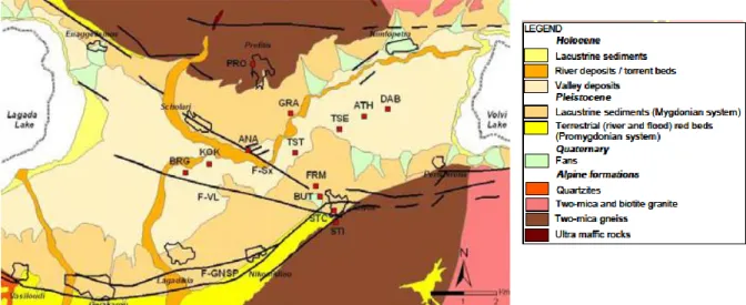
Between 2005 and 2008, the Aristotle University of Thessaloniki, the CEA, the Laue-Langevin Institute, and ISTerre at Joseph Fourier University, jointly organized an international benchmark, called the ―EUROSEISTEST Verification and Validation Project‖ (E2VP-1). This benchmark aimed at (i) evaluating the accuracy of numerical 2D/3D methods implemented in various simulation codes, when applied to realistic basin models (Fig. 1) chosen from the EUROSEISTEST located in the Mygdonian sedimentary basin of the Volvi area, near Thessaloniki (http://euroseis.civil.auth.gr), and (ii) quantitatively comparing the recorded and numerically simulated earthquake ground motions.
Figure 1. Map of the Mygdonian basin (Mountrakis et al., 1997), showing the strong motion array at the free
surface (red squares), the faults (solid black lines) and villages outlines bordering the basin (solid lines).
In this paper, we first present the 2D basin model and associated velocity model used in this study. Then we compare the 2D linear elastic results obtained for three different numerical schemes, namely Finite-Element (FEM), Spectral-Element (SEM) and Finite-Difference (FDM) Methods. Finally, we compare the 2D results with those obtained from 1D wave propagation in two boreholes extracted at the edges of the 2D basin profile, considering elastic, viscoelastic and nonlinear behaviors for soil materials.
2. Numerical simulations
2.1. Introduction
Preliminary E2VP-1 2D computations were designed to be valid up to 8 Hz on a profile extracted between Stivos (STI) and Profitis (PRO) arrays (see Fig. 1), considering different assumptions, in order to assess the effect of: (i) the model geometry (e.g. surface topography), (ii) the velocity model (e.g. internal sediment layering / gradient, bedrock weathering, Poisson ratio) and (iii) the rheological behavior of constitutive materials (e.g. no damping, viscous vs. hysteretic damping). These computations showed large differences among the modeling teams. After further iterations among some of the teams, especially the meshing of the media, significant improvements were achieved to converge to similar synthetic seismograms. Some of these results are
9ème Colloque National AFPS 2015 – IFSTTAR 3
presented in the following sections, as well as a comparison with 1D simulations performed on 2 borehole profiles located near both edges (X = 2700 m and 6300 m) of the 2D basin profile (Fig. 2). The input motions were similar to the ones used for the 2D analyses and were imposed at the base of the soil columns (GL -300m).
2.2. The 2D basin model and velocity structure
The 2D flat profile used for analysis is shown on Figure 2. It included 7 alluvial layers and a bedrock assumed as weathered (WZ) from surface to 80m depth, and un-weathered underneath. The elastic and attenuation features for the profile are recalled in Table 1, respectively for the alluvial layers and bedrock models, considering here constant properties for WZ. Log for the soil columns extracted at boreholes BH1 and BH2 located near both edges of the 2D basin (Fig. 2) are provided in Fig. 3.
Figure 2. Overview of the strong motion array (red: surface instruments; black sq.: borehole accelerometers)
after Manakou et al. (2007) and profiles with alluvial layers (capital letters) and 1D boreholes BH1 and BH2.
Layer VP (m/s) VS (m/s) Density (kg/m3) QS QP 1=A 1500 130 2050 15 75 2=B 1500 200 2150 20 75 3=C 1650 300 2075 30 83 4=D 2050 450 2100 40 103 5=E 2450 600 2155 60 123 6=F 2550 700 2200 70 140 7=G* 3500 1250 2500 100 200 WZ 3500 1250 2500 100 200 Bedrock (un-weathered) 4500 2600 2600 ∞ ∞
Table 1. Main features of the 2D basin profile used for linear analyses -300 -250 -200 -150 -100 -50 0 50 0 20 0 40 0 60 0 80 0 10 00 12 00 14 00 16 00 18 00 20 00 22 00 240 0 26 00 280 0 30 00 320 0 34 00 36 00 38 00 40 00 42 00 44 00 46 00 48 00 50 00 52 00 54 00 56 00 58 00 60 00 62 00 64 00 66 00 68 00 70 00 72 00 74 00 76 00 78 00 80 00 82 00 84 00 86 00 88 00 90 00 92 00 94 00 De pt h (m)
Distance along profile X (m)
Stivos-Profitis 2D flat profile
F G* E D C B A Bedrock (un-weathered) PRO STI NNW SSE WZ WZ BH1 BH2
Figure 3. Log for the 1D soil profiles.
2.3. The input motions
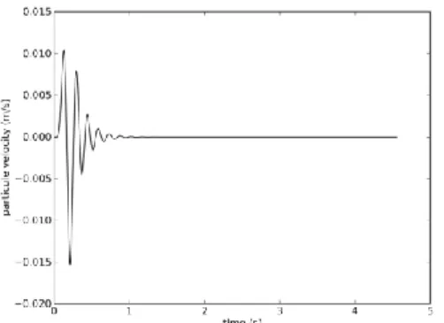
A horizontal pulse corresponding to a SV plane wave with vertical incidence and frequency content between 0 and 8Hz, was set as input motion at the base of the 2D model (GL-300m), scaling input to obtain a PGA for outcropping bedrock motion, of 0.05, 0.1 and 0.25g (e.g. see Fig. 4).
Figure 4. Input pulse velocity corresponding to a 0.1g PGA for outcropping bedrock motion.
2.4. Numerical features
2.4.1. FDM simulations (1D and 2D)
In the FDM simulations, wave equation is solved assuming an isotropic medium and using the stencil of Saenger et al. (2000). In comparison with the classical staggered grid stencil of Virieux (1986), this rotated staggered grid stencil allows using soil parameters such as Lamé parameters and density only once in the numerical stencil, thus avoiding to perform numerical spatial average of these parameters. This stencil property
BH1 B C D E F G* Bedrock (un-weathered) GL-13 (m) GL GL-55.5 GL-75 GL-94 GL-107.5 GL-135.5 GL-300 BH2 B C D E F G* GL-4.5 (m) GL GL-18.5 GL-40.5 GL-55.5 GL-101.5 GL-117.5
9ème Colloque National AFPS 2015 – IFSTTAR 5
has proven to be efficient when modelling the wave propagation in complex media with the presence of cracks (Saenger et al., 2000) or anisotropy (Saenger & Bohlen, 2004). Moreover, stresses and strains share the same location, making easier to implement a non-linear constitutive model in the same way as the Finite-Element Method does. The free surface is introduced by zeroing the Lamé coefficients, corresponding to the vacuum formulation used by Zahradnik et al. (1993) and Saenger et al. (2000). Gelis et al. (2005) showed that this formulation of surface condition in the Saenger's stencil allows to precisely modelling the surface waves propagation. Yet, this stencil requires 15-30 points per minimum Rayleigh wavelength in presence of free surface without topography (Bohlen & Saenger, 2006).
For the 2D simulations, a regular grid spacing of 0.5 m was considered (18 801*700 elements), with 26 points per wavelength, periodic lateral boundary conditions and absorbing boundary at the base of the model (Cerjan et al., 1985). The computing time step was 5.10-5 s. For the 1D simulations, soil columns were simply extracted from the 2D model, assuming identical grid spacing, number of points per wavelength and computing time step.
2.4.2. SEM simulations (2D)
Only 2D simulations were performed in this study with this method, using the 2D version of EFISPEC SEM code (http://efispec.free.fr), which has been widely verified during previous studies (De Martin, 2011; Matsushima et al., 2014; Chaljub et al., 2015; Maufroy et al., 2015). It is based on a continuous Galerkin formulation for solving the weak form of the two-dimensional equation of motion. The numerical scheme follows the one presented by Komatitsch and Tromp (2002). The transient dynamic simulation was designed to be valid up to 10Hz, considering 7 Gauss-Lobatto-Legendre (GLL) points per wavelength and shape functions of order 4. The collocation grid where the equations of motion are solved has 422,354 degrees of freedom. The spatial discretization consisted in an unstructured mesh of 13,118 linear quadrangle elements and 132 line elements (L2) used to model either the absorbing boundary condition at the base of the profile or the periodic lateral boundary conditions. As the bedrock is assumed to remain elastic under dynamic loading, we used absorbing elements based on a paraxial approximation of order 0 (e.g. Clayton & Engquist, 1977), which provides a relative simple way to model the unbounded domain. The time marching is done using an explicit Newmark scheme ( = 0.5, = 0) with a computing time step of 5.10-6 s.
2.4.3. FEM simulations (2D)
2D FEM simulations were performed using the ECP code GEFDYN (http://www.mssmat.ecp.fr/gefdyn). The numerical solution is formulated on the basis of the Terzaghi’s effective stress principle and assumes an undrained deformable isotropic medium with homogeneous layers and bedrock. As for the SEM code, a continuous Galerkin formulation is assumed for solving the weak form of the governing equations. The transient dynamic simulations were designed to be valid up to 8Hz, considering 10 points per wavelength and a total of 92,952 degrees of freedom. Spatial discretization of the medium consisted in an unstructured mesh of 89,900 linear triangle elements (T3) and 263 L2 used to model the absorbing boundary condition at the base of the profile. Absorbing elements based on a paraxial approximation of order 0 were used in this case. Although nonlinear material behavior was not assumed for lateral boundaries, a tied lateral boundary approach was preferred (Zienkiewicz et al., 1988, 1999). An explicit Newmark time integration scheme was used ( = 0.5, = 0.25) with a computing time step of 10-3 s.
2.4.4. Constitutive modelling
Energy dissipation is needed to avoid unrealistic ground motion (e.g. Graves & Pitarka, 2010) and in the case of strong motion propagating on soft soils, the shear strain becomes significant and nonlinear soil behaviour may
take place (e.g. Bonilla et al., 2010). Two broad classes of constitutive models are used in practice: (i) one considers linear material behavior with viscous damping, and (ii) the other uses cyclic nonlinear modelling (mainly elastoplastic rheology). Both classes have been considered in this study.
Regarding class (i), FDM and SEM schemes have used the technique of Liu & Archuleta (2006), which is based on a generalized Maxwell model (e.g. Graves & Day, 2003) to simulate the wave propagation in a viscoelastic medium. In this case, energy is dissipated through the use of memory variables that allow to implementing constant attenuation between 0.01 and 50 Hz through attenuation (quality) factors ranging from 5 to 5000 and being not necessarily equal for shear and compression waves. Conversely, the well-known equivalent linear approach (e.g. Kramer, 1996) was also used in 1D case.
In the present paper, only FDM simulations have considered a constitutive model of class (ii), using the one proposed by Towhata & Ishihara (1985) and Iai et al. (1990), which considers a plane strain multi-spring mechanism and which is able to account for pore pressure and dilatancy effects (Iai et al., 1990). Furthermore, a hyperbolic model for the stress–strain relation (Kondner & Zelasko, 1963) was used and the hysteresis is taken into account by the so-called Generalized Masing Rules operator (Bonilla, 2000; O’Connell et al., 2012).
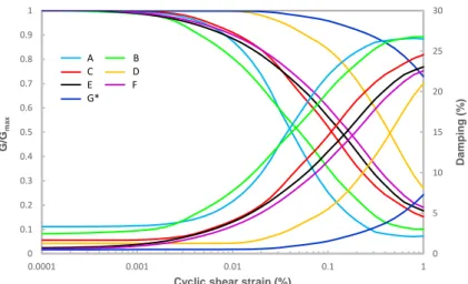
In this study, the linear model considers a constant (initial) shear modulus and damping equal to zero for each layer. The viscoelastic model is similar to the linear one, but with a constant damping equal to 1/(2*Qs). For the viscoelastoplastic model, the linear equivalent approach has used the degradation curves provided by E2VP-1 (see Fig. 5), whereas the FDM scheme has combined the viscoelastic and the elastoplastic (multi-spring) approaches (Gélis and Bonilla, 2012), calibrating the same curves with the hyperbolic model and Generalized Masing Rules. Finally, the pore pressure was neglected in the performed analyses.
Figure 5. Nonlinear E2VP-1 degradation curves.
2.5. Simulation results
We see that FDM, SEM and FEM schemes show a very good agreement for motion computed on rock at the profile edge (Fig. 6). Some improvements in the definition of the mesh that honors the sedimentary layers interfaces are still needed however for the FEM scheme compared to FDM/SEM, which can be seen from the results obtained in the middle of the basin (Fig. 6).
As expected, when comparing 2D and 1D linear surface motion results obtained at the basin edge (Fig. 7), we see that 1D approach is not able to capture surface waves trapped in the basin.
0 5 10 15 20 25 30 0 0.1 0.2 0.3 0.4 0.5 0.6 0.7 0.8 0.9 1 0.0001 0.001 0.01 0.1 1 D amping (% ) G/G m ax
Cyclic shear strain (%)
A B
C D
E F G*
9ème Colloque National AFPS 2015 – IFSTTAR 7
Figure 6. Horizontal surface motions obtained in the basin middle and at the edge, for 2D linear FDM (red),
SEM (blue) and FEM (black) schemes (input pulse motion PGA = 0.05g).
Figure 7. Horizontal BH1 surface motions: comparison between 2D and 1D linear computations for FDM and
SEM schemes (input pulse motion PGA = 0.05g).
Velocity (m/s) Time (s) SEM FDM FEM Velocity(m/s) Time (s) SEM FDM FEM Middle (X = 4400m, sediment)
Horizontal motion at basin surface
Figures 8 and 9 compares 1D results obtained at BH1 or BH2 boreholes, using FDM scheme (in black) and linear equivalent approach (in red), when considering (1) different constitutive models (Fig. 8) or (2) increasing input source magnitudes with the same constitutive model (Fig. 9). In case (1), a perfect match is reached between both approaches, except for the viscoelastoplastic FDM model for which some material nonlinearity is observed while the linear equivalent approach remains linear. In case (2), as expected, the linear equivalent approach is not able to reproduce the nonlinear soil behaviour in the case of strong motion propagating on soft soils.
Figure 8. Horizontal BH1 velocities (m/s) obtained with 1D FDM (black) and linear equiv. (red) approaches,
considering different constitutive models.
Figure 9. Horizontal BH2 velocities (m/s) obtained with 1D viscoelastoplastic model for FDM (black) and
linear equiv. (red) approaches, for the different scaled input pulse motions.
GL-6,5m GL-34m GL-65m GL-85,5m GL-101m GL-122m GL-221m PGA source = 0.05g GL-2m GL-11.5m GL-29.5m GL-48,5m GL-79m GL-110.5m GL-209.5m 0.1g PGA source = 0.05g 0.25g
9ème Colloque National AFPS 2015 – IFSTTAR 9
3. Conclusions
This paper presents the results obtained for the 2D linear case of the E2VP-1 international benchmark (« EUROSEISTEST Verification and Validation Project », 2005-2008), considering three different numerical schemes, namely finite elements (FEM), spectral elements (SEM) and finite differences (FDM) and having achieved later, significant improvements to converge to similar synthetic seismograms. We also present the comparisons between 2D linear results and linear and nonlinear 1D results obtained for soil columns extracted from the 2D basin model.
We have shown that FDM, SEM and FEM schemes are in very good agreement for 2D motions computed on rock at the profile edge. In order to have such agreement, a strong effort was made on the medium meshing, especially to honor the sedimentary layers interfaces. Some improvements are still needed however for the FEM scheme compared to FDM/SEM. Moreover, we show that 1D simulations are no longer valid when multiple surface wave reflections on the basin edges are observed. Finally, as expected, the linear equivalent approach is not able to reproduce the nonlinear soil behaviour in the case of strong motion propagating on soft soils.
4. References
Bohlen, T. & Saenger, E.H., ―Accuracy of heterogeneous staggered grid finite-difference modelling of Rayleigh waves‖, Geophysics, vol. 71, n°4, 2006, p. 109–115.
Bonilla F., Bozzano F., Gélis C., Giacomi A.C., Lenti L., Martoni S. & Semblat J.-F., ―Multidisciplinary study of seismic
wave amplification in the historical center of Rome, Italy‖, 5th Int. Conf. on Recent Advances in Geotech. Earthq.
Engineering and Soil Dynamics, San Diego, CA, May 24–29, 2010.
Bonilla L.F., Computation of linear and nonlinear site response for near field ground motion, PhD thesis, University of California, Santa Barbara, CA, 2000.
Cerjan C., Kosloff D., Kosloff R. & Reshef M., ―A nonreflecting boundary condition for discrete acoustic and elastic wave equation‖, Geophysics, vol. 50, 1985, p. 705–708.
Chaljub, E., Maufroy, E., Moczo, P., Kristek, J., Hollender, F., Bard, P-Y., Priolo, E., Klin, P., De Martin, F., Zhang, Z., Zhang, W., and Chen, X., 3D numerical simulations of earthquake ground motion in sedimentary basins: testing accuracy through stringent models. Geophysical Journal International. 201(1), 90-111.
Clayton R. W. and Engquist B., ―Absorbing boundary conditions for acoustic and elastic wave equations‖, Bull. seism. Soc.
Am., vol. 6, 1977, p. 1529- 1540.
De Martin, F. Verification of a Spectral-Element Method Code for the Southern California Earthquake Center LOH.3 Viscoelastic Case, Bull. Seism. Soc. Am. Vol. 101(6): 2855-2865, December 2011, doi: 10.1785/0120100305
Gélis C. and Bonilla L. F., ―2-D P–SV numerical study of soil–source interaction in a non-linear basin‖, Geophys. J. Int., 191: 1374–1390, doi: 10.1111/j.1365-246X.2012.05690.x, 2012.
Gélis C., Leparoux D., Virieux J., Bitri A., Operto S. & Grandjean G., ―Numerical modelling of surface waves over shallow cavities‖, J. Environ. Eng. Geophys., vol. 10, 2005, p. 49–59.
Graves R.W. & Day S., ―Stability and accuracy analysis of coarse grain viscoelastic simulations‖, Bull. seism. Soc. Am., vol. 93, n°1, 2003, p. 283–300.
Graves R.W. & Pitarka A., ―Broadband ground motion simulation using a hybrid approach‖, Bull. seism. Soc. Am., vol. 100, n°5A, 2010, p. 2095–2123.
Iai S., Matsunaga, Y. & Kameoka T., ―Strain space plasticity model for cyclic mobility‖, Rep. Port Harbour Res. Inst., vol. 29, 1990, p. 27–56.
Komatitsch, D., and J. Tromp. Spectral-element simulations of global seismic wave propagation—I. Validation, Geophys. J. Int. 149, 2002, 390–412, doi 10.1046/j.1365-246X.2002.01653.x.
Kondner R.L. & Zelasko J.S., ―A hyperbolic stress-strain formulation for sands‖, 2nd Panamerican Conf. on Soil Mechanics and Found. Engineering, 1963, p. 289–324.
Kramer S., ―Geotechnical Earthquake Engineering‖, Prentice Hall, 1996.
Liu P.C. & Archuleta J.R., ―Efficient modeling of Q for 3D numerical simulation of wave propagation, Bull. seism. Soc. Am., vol. 96, n°4A, 2006, p. 1352–1358.
Manakou M., Raptakis D., Apostolidis P., Chavez Garcia F.J., Pitilakis K., ―The 3D geological structure of the Mygdonian
sedimentary basin (Greece)‖, 4th Int. Conf. on Earthq. Geotech. Engineering, 4ICEGE, Thessaloniki, June 25-28, 2007,
Paper No. 1686.
Matsushima, S., T. Hirokawa, F. De Martin, H. Kawase, F. J. Sánchez-Sesma. The Effect of Lateral Heterogeneity on Horizontal-to-Vertical Spectral Ratio of Microtremors Inferred from Observation and Synthetics Bulletin of the Seismological Society of America, vol. 104(1):381-393, February 2014, doi:10.1785/0120120321
Maufroy, E., E. Chaljub, F. Hollender, J. Kristek, P. Moczo, P. Klin, E. Priolo, A. Iwaki, T. Iwata, V. Etienne, F. De Martin, N. Theodoulidis, M. Manakou, C. Guyonnet-Benaize, K. Pitilakis, and P.-Y. Bard, Earthquake ground motion in the Mygdonian basin, Greece: the E2VP verification and validation of 3D numerical simulation up to 4 Hz. Bulletin of the Seismological Society of America. 2015.
Mountrakis D., Kilias A., Pavlides S., Sotiriadis L., Psilovikos A., Astaras Th., Vavliakis E., Koufos G., Dimopoulos G., Soulios G., Christaras V., Skordilis M., Tranos M., Spiropoulos N., Patras D., Sirides G., Lambrinos N., Laggalis Th., ―Special edition of the neotectonic map of Greece‖, Earthquake Planning and Protection Organization (OASP), 1997 (in Greek).
O’Connell D.R.H., Ake J.P., Bonilla F., Liu P., La Forge R. & Ostenaa D., ―Strong ground motion estimation‖, in Earthquake Research and Analysis—New Frontiers in Seismology, ed. Sebastiano D’Amico, In-Tech, ISBN: 978–953-307–840-3. 2012.
Saenger E., Gold, N. & Shapiro, S., ―Modeling the propagation of elastic waves using a modified finite-difference grid‖,
Wave Motion, vol. 31, 2000, p. 77–82.
Towhata I. & Ishihara K., ―Modeling soil behavior under principal axes rotation‖, 5th Int. Conf. on Numerical Methods in
Geomechanics, Nagoya, Japan, 1985, p. 523–530.
Virieux J. ―P-SV wave propagation in heterogeneous media: velocity-stress finite-difference method‖, Geophysics, vol. 51, n°4, 1986, p. 889–902.
Zahradnik J.P., Moczo P. & Hron F., 1993. ―Testing four elastic finite difference schemes for behaviour at discontinuities‖,
Bull. seism. Soc. Am., vol. 83, 1993, p. 107–129.
Zienkiewicz O., Bicanic N. and Shen F., ―Earthquake input definition and the transmitting boundary conditions‖, In
Doltsinis, I. S., editor, Advances in Computational Nonlinear Mechanics, 1988, p. 109-138.
Zienkiewicz O., Chan A., Pastor M., Schrefler B. and Shiomi T., Computational Geomechanics with Special Reference to