HAL Id: cea-02437054
https://hal-cea.archives-ouvertes.fr/cea-02437054
Submitted on 13 Jan 2020
HAL is a multi-disciplinary open access
archive for the deposit and dissemination of
sci-entific research documents, whether they are
pub-lished or not. The documents may come from
teaching and research institutions in France or
abroad, or from public or private research centers.
L’archive ouverte pluridisciplinaire HAL, est
destinée au dépôt et à la diffusion de documents
scientifiques de niveau recherche, publiés ou non,
émanant des établissements d’enseignement et de
recherche français ou étrangers, des laboratoires
publics ou privés.
convection sodium flow
U. Bieder, L. Ishay, G. Ziskind, A. Rashkovan
To cite this version:
U. Bieder, L. Ishay, G. Ziskind, A. Rashkovan. CFD analysis and experimental validation of mixed
convection sodium flow. International Congress on Advances in Nuclear Power Plants (ICAPP 2017),
Apr 2017, Fukui And Kyoto, Japon. �cea-02437054�
CFD ANALYSIS AND EXPERIMENTAL VALIDATION OF MIXED CONVECTION SODIUM FLOW
Bieder U.
DEN-STMF, CEA, Université Paris-Saclay, 91191 Gif-sur-Yvette, France, [email protected]
Ishay L. and Ziskind G.
Department of Mechanical Engineering, Ben-Gurion University of the Negev, Beer-Sheva 84105, Israel
Rashkovan A.
Physics Department, Nuclear Research Center Negev, 84190 Beer-Sheva, Israel
Formation and destruction of thermal stratification can occur under certain flow conditions in the upper plenum of sodium cooled fast breeder reactors (SFR). The flow patterns in the hot sodium pool of the upper plenum are very complex, including zones of free and wall-bounded jets, recirculation and stagnation areas. The interaction of the sodium flow and thermal stratification has been analyzed experimentally at CEA in the years 1980-1990 in the SUPERCAVNA facility. The facility consists of a rectangular cavity with temperature-controlled heated walls where the flow is driven by a wall-bounded cold jet at the bottom of the cavity. Experimental data of the temperature distribution in the cavity are available for steady-state and transient flow conditions. The experiments are analyzed with the CEA CFD reference code TrioCFD and the commercial code FLUENT by using Reynolds Averaged Navier-Stokes (RANS) equations.
It is shown that a two-dimensional treatment is sufficient for the analysis of steady-state SUPERCAVNA experiments. It is necessary to take into account correctly the conjugate heat transfer between walls and cavity. Turbulence modelling with k- models, in either standard, realizable or RNG formulations, does not lead to significant differences in the calculated temperature fields which are in good accordance to the measurements. Different wall treatments also do not change these results. Thus, it seems that turbulence modelling is not a predominant factor in a successful simulation of the mixed convection experiments. However, using temperature-dependent physical properties is a very important factor in simulating the experiments correctly, although the Boussinesq approximation is justified. Finally, it is shown that a three-dimensional treatment is necessary for the analysis of transient experiments.
I. INTRODUCTION
The three sodium cooled fast breeder reactors (SFRs) Rapsodie, Phénix and Superphénix have been built in
France in the last 50 years. France was also engaged in collaboration with the United Kingdom and Germany in the European Fast Reactor project, launched for several years in the late 1980s. Many thermal-hydraulic studies were performed to support design and safety analysis for Superphénix and then for the European FR project1.
Initially based on analytical and experimental means, thermal-hydraulic studies also progressively included numerical simulation.
The study presented here concerns a temperature-stratified liquid sodium flow which may establish under certain operating conditions in the upper plenum (also called hot pool) of pool type SFRs. The experimental work was initiated in the early 1970s in connection with the Phénix and Superphénix plants2. Liquid sodium
coolant is circulating in the upper plenum as shown in Fig. 1.
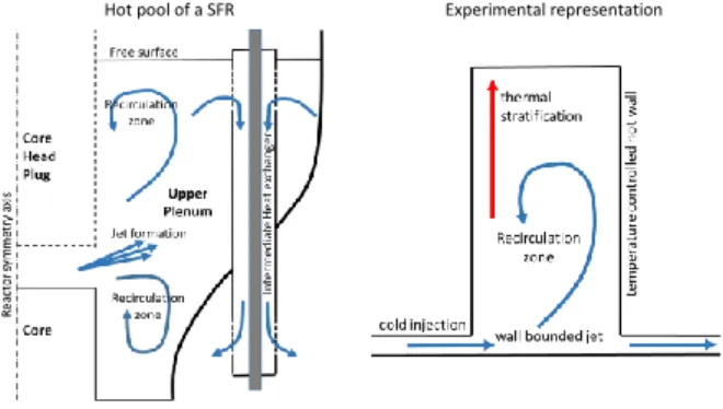
Fig. 1: Flow in the hot pool of a SFR (left) and its simplified experimental representation (right).
The core delivers hot sodium beneath the core head plug. The flux is deflected vertically and transported to the intermediate heat exchangers (IHX) at the other end of the upper plenum, where it is driven by natural convection through the IHX to the lower plenum. The flow conditions in the plenum are highly complex, involving jet- and recirculating zones, where the sodium flows at
velocities which are significantly lower than its main-stream velocities near the core outlet.
During certain operating transients, the core outlet temperature may change rapidly with time; an emergency shutdown for example results in a sharp temperature reduction. These temperature variations result in density changes which may affect flow conditions, particularly in regions of low velocities. Buoyancy effects may cause thermal stratification characterized by fluid distribution into layers with increasing temperature from the bottom up. Once established, stratification conditions may last for a long time2.
In order to understand the physical phenomena in the upper plenum, thermal-hydraulic studies use two complementary approaches to predict realistically temperature distribution and flow fields:
Numerical models capable of simulating multi-dimensional flow with complex geometries and multiple physical effects;
Reduced-scale experimental models using liquid sodium or simulating fluids.
The numerical and experimental model approaches are both approximate. The accuracy of computer codes depends on the mathematical modelling, particularly the modelling of turbulence in stratified flows of liquid metals. In numerical studies, the physical modelling should respect all non-dimensional numbers, and that can be an impossible task for sodium flow due to its low Prandtl number. Thus, it is necessary to perform experiments with sodium to approach the real SFR plant conditions.
A simplified experimental representation of the upper plenum of a pool type SFR is shown on the right of Fig. 1. It is using the simple geometrical configuration of a rectangular, temperature-controlled cavity. This set-up involves the two most essential phenomena occurring in the plenum:
Thermal stratification imposed by the heated wall and Recirculation zones, imposed by the wall jet.
II. The SUPERCAVNA facility II.A Geometry
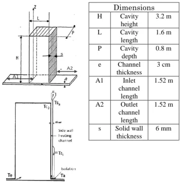
The SUPERCAVNA facility consisted of a rectangular cavity as shown in Fig. 2, connected at the bottom to rectangular inlet and outlet channels. All the walls of cavity and channels are thermally isolated. Two distinct sodium test loops are operated to control the temperature and flow conditions independently in the inlet channel and the side-wall heating channel2. The flow
forced into the inlet channel induces a recirculating flow in the cavity. The velocity profile at the exit of the inlet channel was assumed to be hydraulically fully- developed
for the range of conditions studied, which is not totally the case for an inlet length A1 of about 50e, where “e” is the channel thickness.
Dimensions H Cavity height 3.2 m L Cavity length 1.6 m P Cavity depth 0.8 m e Channel thickness 3 cm A1 Inlet channel length 1.52 m A2 Outlet channel length 1.52 m s Solid wall thickness 6 mm
Fig. 2: SUPERCAVNA test section and geometry.
For the vertical wall heating, the inlet of the side-wall heating channel is located at mid-height of the cavity. Sodium is conveyed to the bottom of the heating element, turns upwards, and then exits at the top. At the bottom, a 20 mm gas jacket limits heat transfer to the channel.
II.B Physical properties
The physical properties of liquid sodium are given in Table 1 for the temperature range of 500K to 600K. Physical properties of the solid structures of the facility are also added to this table.
TABLE 1: Physical properties of sodium and INOX.
Material Unit Sodium INOX Temperature 500 600 500 600 Density kg/m3 897 874 8000 8000 Dynamic viscosity Pa s 4.15 *104 3.21 *104 - - Thermal conductivity W/m/K 80.1 73.7 18 18 Specific heat capacity J/kg/K 1334 1301 480 480 Thermal expansion coefficient 2.50 *104 2.60 *104 - -
II.C Selected SUPERCAVNA experiments
Besides the physical properties and length scales defined above, flow parameters are related to velocity and temperature scales in order to define three non-dimensional numbers: Reynolds Number: 𝑅𝑒 =𝜌0∙𝑉0∙𝐿 𝜇0 Richardson Number: 𝑅𝑖 =𝑔∙𝛽∙∆𝑇∙𝐿𝑉 02 (1) Péclet Number: 𝑃𝑒 =𝜌0∙𝐶𝑝0∙𝑉0∙𝐿 𝜆0
The subscript 0 defines the average value in the inlet channel. Thus, V0 is the average flow velocity in the test
section inlet channel. We note that:
In the steady-state case, T represents the difference between the maximum temperature at the heating wall and the temperature at the channel inlet (Tc2-Te
in Fig. 2).
In the transient case, T corresponds to the magnitude of the temperature drop between the channel inlet and cavity in initial state.
II.C.1 Steady state experiments
In the steady state case, a two-step experimental procedure is used:
1. Sodium flowrates in both cavity inlet channel and wall heating channel are stabilized at the same initial temperature;
2. At constant flow rates, the temperature in the heating channel is raised to the target value while the cavity loop temperature is maintained at its initial value.
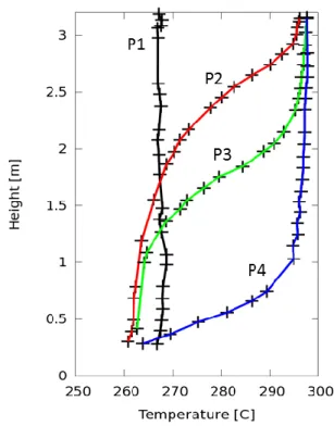
Fig. 3 shows measured temperature profiles along the vertical axis (0<y<3.23) at the center of the cavity (z=0.4), 0.1 m from the left cavity wall. Selected experiments with increasing values of the Richardson number and decreasing value of the Péclet Number are shown, as given in Tab.2:
TABLE 2: Non-dimensional numbers characterizing the steady state experiments
.
The experiments go from pure convection-controlled conditions (P1) over mixed convection (P2, P3) to pure buoyancy- controlled conditions (P4). Only the mixed convection experiments are analyzed herein.
II.C.2 Transient experiments
Under transient conditions, only cold thermal shocks in the cavity can be simulated. In such cases, the side-wall heating system is drained. The procedure is as follows:
1. The flowrate and the temperature in the cavity are stabilized at initial conditions;
2. Activating the sodium-air heat exchanger in the main loop, the temperature in the cavity inlet channel can be modified at constant flow rate.
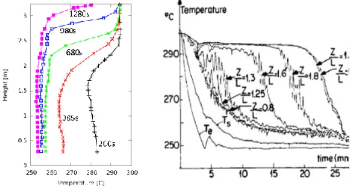
Only one experiment under mixed convection conditions is analyzed, with Ri of 0.3 and Pé of 20,000. The temporal development of vertical temperature profiles and local temperature time evolution at various heights in the cavity are shown in Fig. 4. The local temporal evolution at six elevations (Z/L) in the center of the cavity is shown on the left of Fig. 4. Te and Ts are explained later.
Test case Péclet Number Richardson Number
P1 41000 0.03
P2 22000 0.19
P3 16000 0.36
P4 6900 2.20
Fig. 3: Comparison of measurement and calculation at x=0.1m (TrioCFD).
Fig. 4: Transient experiment; variation of vertical temperature profiles with time (left) and local temperature
course at selected heights in the cavity (from ref.(3)).
The cold shock transient can be divided into three main consecutive stages:
Stage l: first 2.5 minutes:
The cavity is initially isothermal (T= 300°C). The incoming sodium does not yet show buoyancy effects, is momentum driven and mixes with the sodium of the cavity, up to the cavity top.
Stage II: from 2.5 minutes to 7 minutes:
In this stage, the buoyancy effects significantly modify the dynamic field, as buoyancy opposes the initial momentum. A new flow pattern appears, which is characterized by a small recirculating eddy in the lower part of the cavity.
Stage III: final 15 minutes:
This stage is characterized by erosion of the thermal stratification by the cold sodium flow. The hot/cold interface moves slowly upward, towards the top of the cavity.
III. NUMERICAL APPROACH
In Reynolds-averaged approaches to turbulence, the non-linearity of the Navier-Stokes equations gives rise to Reynolds stress terms that are modeled by turbulence models. Almost all turbulence models for industrial applications are based on the concept of eddy-viscosity for the Reynolds stress. This approach leads in matrix notation to: ij i j j i T j i k x U x U u u 3 2 ' '
(2)
The following Reynolds-averaged mass conservation equation, Navier-Stokes equations (RANS) and energy conservation equation are solved for incompressible flows
by using the Boussinesq approximation to account for thermal effects: 0 j j x U , (3)
i i j j i T j i j j i i T T g x U x U x x P x U U t U 0 1
j t j j j x T a a x x T U t T . (5)Explicit dependence of sodium density on temperature was also employed. In this case the Boussinesq approximation in the momentum equation is relaxed. :
III.A TrioCFD simulations
In the study presented here, the turbulent viscosity is calculated from the well-known k- model by using the following formulation:
2 k C t (6)G
P
x
k
x
x
k
U
t
k
j k t j j j
)
(
(7) k G C C k C k P C x x x U t j t j j j 3 2 2 1 ) ( j i j i x U u u P ' ' , with ui'uj' calculated by eq. (2) and
T g G j t t Pr (9)
The following empirical coefficients are used: C=0.09, k=1, =1.3, C1=1.44, C2=1.92. C3 is set to
unity for stable thermal stratification and zero for unstable stratification.
Standard wall functions are used to model momentum exchange between wall and fluid. The general wall law of Richardt4 with (=0.415) is used to account
for viscous, buffer and logarithmic law regions:
11 3 11 1 44 . 7 1 ln 1 y e y y e y u (10)Two modifications of this standard model are applied in sensitivity studies presented here:
For fluids with low Pr numbers as sodium, the turbulent thermal diffusivity at can be calculated from
t p t t c a 85 . 0 7 . 0 2 (11)
As linear eddy viscosity models cannot account for anisotropic turbulence, characteristic to thermally stratified flows, a non-linear eddy viscosity model is applied, where an additional non-linear term is added to the Reynolds stress term6:
NL ij ij i j j i T j i k x U x U u u 3 2 ' ' (12)
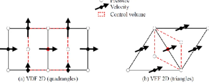
The spatial discretization in TrioCFD is the classical staggered grid finite-volume differences method7 (VDF)
for rectangles (2D) and hexahedra (3D), as well as the extension of this method to triangles (2D) and tetrahedrons (3D) by means of a hybrid finite-volume element method8 (VEF). In VDF, the velocity is located at
the centers of the faces while pressure and scalars are located at the center of the element. In the VEF, velocity and scalars are located at the center of the faces and the pressure is located at both the center of the element and the element vertices. This is shown schematically in Fig. 5. More information on the TrioCFD code can be found in ref.(9).
Fig. 5: Schematic representation of discretization methods with momentum control volumes.
III.B FLUENT simulations
The collocated finite-volume formulation of the conservation laws is solved in FLUENT10. Three
variances of k- model were employed: standard, RNG11
and realizable12. The three models solve transport
equations for turbulent kinetic energy, k, and its dissipation rate, . Generation of turbulent kinetic energy in the presence of buoyancy is expressed as presented in eq. (9) above. Heat transfer is modelled using Reynolds analogy of heat and momentum transfer. All the models were used along with the high y+ law of the wall
formulation for resolving heat and momentum transfer at the walls of the cavity.
The 2D simulations were run in transient mode until a steady state was reached. The presented results were obtained on a verified grid;
a solution with the grid twice finer in each direction (quadrupled number of cells) was found to be identical to the one obtained with the initial grid.
IV. Numerical Results
IV.A Specification of modelling hypothesis
Numerous tests have been made with FLUENT and TrioCFD in order to define an optimal modelling strategy.
IV.A.1 Flow boundary conditions
A contraction is present in the inlet channel about 25 hydraulic diameters (50e) upstream of cavity inlet. Thus, a constant velocity in space is imposed at the inflow-channel inlet. Analogously, k and are estimated for fully developed channel flow and imposed as constant in space. Pressure imposed free outflow conditions are used at the outlet channel exit. Wall functions are used at all walls of the inlet and outlet channels, as well as of the cavity itself.
IV.A.2 Thermal boundary conditions
Adiabatic walls are assumed for all walls except for the heated side wall. In order to ensure an almost constant temperature in the side-wall heating channel, the same mass flow rate was imposed experimentally in the side-wall heating channel and the cavity. This equal distribution of the sodium flow into the two loops led to temperature differences of 3 to 10K between inlet and outlet of the side-wall heating channel. Preliminary numerical tests have shown that Dirichlet thermal boundary conditions with an imposed constant or linear wall temperature at the heated side wall do not lead to the observed temperature stratification. In fact, it is necessary to model the conjugate heat exchange between cavity, solid wall and side-wall heating channel.
IV.A.3 Physical properties
Further numerical tests have shown that only using the Boussinesq approximation to account for thermal effects is not sufficient to reproduce the experimental results. Rather, sodium kinematic viscosity , thermal conductivity and thermal expansion coefficient must be taken as temperature dependent.
IV.A.4 Meshing
Based on convergence tests of Gurgacz13 with 29k,
58k and 116k meshes, a reference 2D conforming mesh with 160×335 rectangles in the cavity has been defined for calculations with wall functions. Inlet and outlet
channels were discretized each with 150×15 rectangles. This reference mesh leads to y+ values of about 50 in the
inlet and outlet channels and of about 25 in the cavity close to the heated side wall. For sensitivity calculations of the discretization method, each rectangle was cut into two triangles in order to create a fully triangular meshing. These meshes are shown in Fig. 6 with zooms of the inlet channel entry to the cavity. For 3D calculations, 80 meshes were added in span-wise direction, leading to 9.28 million parallelepiped elements.
Fig. 6: Basic 2D meshes on rectangles and triangles.
IV.B Steady state experiment
As discussed in chapter 3.1, a two-step procedure is used to achieve experimentally steady state conditions. This procedure has required up to 24 hours to fully stabilize the temperature in the cavity. For the numerical analysis, a “faster” procedure was used.
1. The cavity is initialized with hot stagnant sodium; at the inflow channel inlet, cold sodium is imposed at final velocity.
2. The heating channel is initialized with hot sodium at final velocity; at heating channel inlet, hot sodium is imposed at final velocity.
3. A transient, under constant boundary conditions, is calculated until the stratification layer is not moving any more.
The thermal-hydraulic inflow conditions at the cavity inlet channel and the side-wall heating channel are given in Table 3 for the steady state experiment P3.
TABLE 3: Input data for steady state experiment P3.
The resulting temperature distribution in the cavity is shown in Fig. 6 (TrioCFD; VDF; Prt = 0.9). The
stratification interface is at about 2 m height. The presence of the cold wall-bounded jet at the cavity bottom
is clearly visible, as well as the erosion of the thermally stratified layer by the flow ascending the heated side wall. This ascending flow is accelerated by buoyancy, initiated by the hot side-wall heating channel. The axial temperature profile in the cavity close to the side-wall and in the heated channel is added to Fig. 7. The temperature in the channel decreases up to the stratification interface and increases above it to the temperature cavity top.
Fig. 7: Temperature distribution in the cavity and the side-wall heating channel.
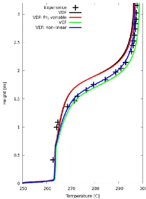
Comparisons of measured vertical temperature profiles are shown in Fig. 8 for the distance of 0.1m from the left, adiabatic, cavity wall. It can be seen that:
Temperature field Temperature at heated side wall
Mean velocity inlet channel V0 m/s 0.69
Mean velocity heating channel Vh m/s 0.69
Mean temperature inlet channel Te °C 250.0
Mean Temperature heating channel Tsi °C 303.1
Fig. 8: Comparison of measurement and calculation at
VDF slightly overestimates the height of the stratification interface, independently of the modelling method for the turbulent Prandtl number. This is most probably related to the fact that flow in the main axial direction is slightly overestimated with this kind of discretization. Thus, the upward buoyancy- driven flow at the heated side wall might be overestimated with Uy=0.218m/s. This enhanced
upward velocity overestimates the erosion of the stratified layer.
VEF predicts correctly the height of the stratification interface, where the non-linear turbulence model leads to a slightly higher located stratification layer. It seems that anisotropic turbulence plays a certain but not dominant role in this experiment. With a maximal vertical velocity near the heated side wall of
Uy=0.208m/s, the result is slightly lower than in VDF
discretization.
Although VEF with a non-linear eddy viscosity model seems to represent the SUPERCAVNA experiment very well, it is not evident that this method outplaces VDF in all cases.
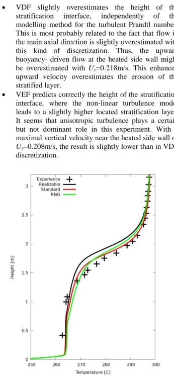
The influence of the turbulence model has been analyzed with the FLUENT code. Comparisons with measured vertical temperature profile are shown in Fig. 9 for the distance of 0.1 m from the left, adiabatic, cavity wall. It can be seen that:
The temperature distribution calculated with the standard k- model and using standard wall functions gives close results for the two codes (TrioCFD and FLUENT).
Differences between the standard model and RNG
k- are very small.
The realizable k- model predicts a slightly higher stratification interface than measured.
IV.C Transient experiment
As discussed in chapter 3.2, a two-step procedure is used to perform the transient experiment. Self-evidently, this procedure is followed in the calculation. The side-wall heating channel is disconnected from the calculation domain and all side wall is assumed to be adiabatic. As an initial condition, the temperature and flowrate in the cavity are stabilized by a preliminary transient of 200 s with a constant velocity (0.825 m/s) and temperature (300 °C) at the cavity inflow channel inlet. Then, when the sodium/air heat exchanger is operated, the temperature at the inlet channel decreases exponentially in about 240 s from 300 °C to 250 °C, as can be seen from Fig. 4. This temperature decrease is modelled by the correlation:
Te = -3.129559*10-6*t3 + 1.858676*10-3*t2 – 0.4742906*t + 300.0347
The resulting transient temperature distribution in the cavity is shown in Fig. 10 for eight different instants at the beginning of the transient (TrioCFD; VDF; Prt = 0.9).
The three experimentally detected stages (chapter 3.2) can be distinguished:
Fig. 10: Development of the temperature distribution in the cavity.
Stage I:
At the beginning of the transient, 3D effects are clearly visible in the temperature field close to the side-wall at which the cold jet impinges. A cold “tongue” develops along the wall and leads until 80 seconds to a complete Fig.9: Comparison of measurement and calculation at
mixing within the cavity. Buoyancy effects are negligible during this period.
Stage II:
Stratification starts to develop at about 100 s due to increasing buoyancy effects. Complex flow structures develop in both fluid layers: the upper, hot and stratified layer and the lower colder well-mixed layer.
Stage III:
At about 480 s, a distinct stratification is present with a stagnant flow in the upper hot layer and large circulation in the lower colder layer.
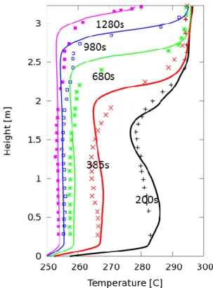
The measured temporal development of the axial temperature profile (0<y<3.23) located at the center of the cavity (x=0.8m, z=0.4m) is compared in Fig. 11 to the corresponding calculated profiles. The calculated profiles at 200 s and 385 s seem to be more variable than the measured ones. This might be an indicator that the thermal boundary condition during the initial part of the transient, defined by eq. (12), does not represent completely correctly the initial transient. Unfortunately, more information on this part of the transient is not available.
After about 480 s, when the stratification interface develops slowly upward, the calculation represents well the experiment. During this period the stratification is
eroded slowly by the cold fluid impacting on the interface.
V. CONCLUSION
Formation and destruction of thermal stratification can occur under certain flow conditions in the upper plenum of sodium cooled fast breeder reactors (SFR). The interaction of the sodium flow and thermal stratification has been analyzed experimentally at CEA in the years 1980-1990 in the SUPERCAVNA facility. The facility consists of a rectangular cavity with temperature-controlled heated walls where the flow is driven by a wall-bounded cold jet at the bottom of the cavity. The experiments are analyzed with the CFD codes TrioCFD and FLUENT by using Reynolds Averaged Navier-Stokes (RANS) equations.
It is shown that a two-dimensional treatment is sufficient for the analysis of steady-state SUPERCAVNA experiments. It is necessary to take into account correctly the conjugate heat transfer between walls and cavity. Turbulence modelling with k- models, in either standard, realizable or RNG formulations, does not lead to significant differences in the calculated temperature fields which are in good accordance to the measurements. Different wall treatments also do not change these results. Thus, it seems that turbulence modelling is not a predominant factor in a successful simulation of this mixed convection experiments. However, using temperature-dependent physical properties is a very important factor in simulating the experiments correctly, although the Boussinesq approximation is justified. Finally, it is shown that a three-dimensional treatment is necessary for the analysis of transient experiments.
REFERENCES
1. Tenchine D., “Some thermal hydraulic challenges in sodium cooled fast reactors”, Nuclear Engineering
and Design, 240, 1195–1217 (2010)
2. Vidil R., D. Grand and F. Leroux, “Interaction of
recirculation and stable stratification in a rectangular cavity filled with sodium”. Nuclear Engineering and
Design, 105, 321-332 (1988)
3. Kays W. M., “Turbulent Prandtl Number: Where are we?” Transactions of the ASME Journal of Heat
Transfer, 116, 284-295 (1994)
4. Vidil R., J.C. Astegiano, D. Grand and A. Marechal, “Experimental and numerical studies of mixed convection in a cavity, Cases of sodium and water”,
7th International Heat Transfer Conference, Munich
(1981)
5. Hinze J.O., “Turbulence”, McGraw-Hill (1959) 6. Baglietto E., H. Ninokata, “A turbulence model study
for simulating flow inside tight lattice rod bundles”. Fig. 11: Comparison of measurement and calculation at
Nuclear Engineering and Design, 235, 773–784
(2005)
7. Harlow, F.H., Welsh, J.E., “Numerical calculation of time dependent viscous incompressible flow with free surface”. Phys. Fluids, 8, 2182-2189 (1965) 8. Émonot P., « Méthodes de volumes éléments finis :
applications aux équations de Navier-Stokes et résultats de convergence », PhD thesis, Université Lyon I (1992)
9. Angeli P.-E., Bieder U., Fauchet G., “Overview of the Trio_U code: Main features, V&V procedures and typical applications to engineering”,
NURETH-16, Chicago, USA, (2015)
10. ANSYS Fluent User's Guide. Release 15.0. ANSYS Inc.
11. Yakhot, V., Orszag, S.A., Thangam, S., Gatski, T.B. & Speziale, C.G., “Development of turbulence models for shear flows by a double expansion technique”, Physics of Fluids A, 4, 7, 1510-1520 (1992)
12. Shih T.-H., W. W. Liou, A. Shabbir, Z. Yang, and J. Zhu, “A New k- Eddy-Viscosity Model for High Reynolds Number Turbulent Flows - Model Development and Validation”, Computers Fluids,
24(3), 227-238 (1995)
13. Gurgacz S., U. Bieder, Y. Gorsse, K. Swirski, “CFD Simulations of Selected Steady-State and Transient Experiments in the PLANDTL Test Facility”. 7th
European Thermal-Sciences Conference, Krakow,