by
Eugene M. Rasmusson B. S., Kansas State University
(1950)
M. S., St. Louis University (1963)
SUBMITTED IN PARTIAL FULFILLMENT OF THE REQUIREMENTS FOR THE
DEGREE OF DOCTOR OF PHILOSOPHY at the MASSACHUSETTS INSTITUTE of TECHNOLOGY May, 1966 Signature of Author. Certified by ... .... .. - . . 4...., 0--o 2.-.. ...
Department of Meteorology, 13 May 1966
. ... r...
Thesis Supervisor
Accepted by... . . .
by
Eugene M. Rasmusson
Submitted to the Department of Meteorology on 13 May 1966 in partial fulfillment of the requirements for the degree of
Doctor of Philosophy.
ABSTRACT
The atmospheric water vapor flux and certain aspects of the water balance over the North American Sector are investigated for
the period May 1, 1961 - April 30, 1963.
The vertical variation of the flux, as well as the total vertically integrated flux, are investigated from mean monthly data. The flux exhibits important diurnal variations, particularly during the summer south of 500N. These variations are primarily the result of diurnal variations in the mean wind, rather than in the moisture, and are par-ticularly well organized over eastern North America, the Gulf of
Mexico, and the Caribbean Sea.
Significant interannual changes in the flux are also observed. The relationship of these changes to the interannual changes in flux divergence and precipitation are discussed.
The mean vertical distribution of flux divergence is computed for the United States, for the months of January and July. Strong flux convergence in the lowest 100 mb, and divergence in the remainder of the troposphere, was found in July. Flux convergence was found
throughout the troposphere in the east in January, with a maximum be-tween 900 and 950 mb, while in the west convergence (with no particu-larly pronounced maximum) was found above 800 mb, with weak diver-gence below. Corresponding features of the profiles were found at higher elevations over the west, where the flux divergence above 500 mb is quite significant.
Particular emphasis is placed on computations of the vertically integrated vapor flux divergence, and its use in estimating E- , the
mean difference between evaporation and precipitation. Water balance studies, using twice daily observations from the existing aerological
network, indicate that reliable mean annual, seasonal, and monthly values of E-P can usually be obtained for areas of 20 x 105 km2 or larger. The results usually deteriorate rapidly as the size of the area is reduced to less than 10 x 105 km2. This deterioration is primarily the result of a systematic error pattern, which is tentatively ascribed to the effect of diurnal flux variations, small scale features in the mean flux field, and local station peculiarities.
The annual and seasonal values of E-P are computed for the Caribbean Sea and the Gulf of Mexico and are in excellent agreement with independent estimates.
Mean values of E-P are computed for North America north of the United States-Mexican border, and individually for the major water-sheds of the continent. Latitudinally averaged values show a minimum between 550N and 650N.
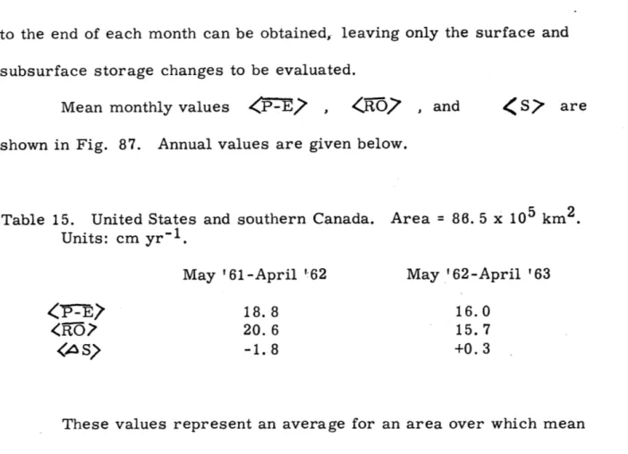
More comprehensive balance studies were made over the United States and southern Canada. Of particular interest is the computation of mean monthly surface and subsurface storage changes directly from measured streamflow and vapor flux data. Consistent and reasonable storage changes are computed for the area as a whole, which indicate an average seasonal variation of around 8 cm. Little net storage change was computed during the two year period for the whole area, but
sub-stantial changes were indicated over the western part of the region during the first year, and over the eastern part during the second year. These
changes appear to be in qualitative agreement with independent indicators. Rough computations of mean monthly evapotranspiration are
made for the United States and southern Canada, using precipitation
and flux divergence data. Values exhibit the expected seasonal variations, with a maximum of around 8 cm/mo in summer and a minimum of 1-2
cm in winter. Computations for the larger subdivisions of this area give values which appear, for the most part, to be reasonable.
Thesis Supervisor: Victor P. Starr Title: Professor of Meteorology
TABLE OF CONTENTS
I. INTRODUCTION ... ... 1
II. REVIEW OF PREVIOUS VAPOR FLUX INVESTIGATIONS ... 11
III. FORMULATION OF THE BALANCE EQUATIONS... 16
IV. DATA AND PROCEDURES... 23
V. REPRESENTATIVENESS OF DATA AND ANALYSES ... 31
A. Representativeness of water vapor flux data... ... 31
B. Representativeness of streamflow data... 38
C. Representativeness and uniqueness of the analyses ... .38
VI. THE LARGE SCALE FEATURES OF THE NORTHERN HEMISPHERE VAPOR FLUX FIELD... 43
VII. THE VERTICAL DISTRIBUTION OF VAPOR FLUX DIVERGENCE OVER THE UNITED STATES... ... 51
VIII. DIURNAL VARIATIONS OF THE WATER VAPOR FLUX ... ... 59
IX. THE ATMOSPHERIC WATER BALANCE OF THE CENTRAL AMERICAN SEA ... ... 79
X. THE WATER BALANCE OVER NORTH AMERICA... 93
A. Introduction ..,... ... ... ... ... 93
B. North American Water Balance... . ... .... 93
C. Northern North America ... . ... 97
1. Water balance... 97
2. Vapor flux ... .. ... ..98
D. United States and Southern Canada .. ... ... 101
1. Introduction... ... ... ... 101
2. Vapor flux... . ... .... 101
3. Water balance ... .... ... 107
E. Central Plains and Eastern Region-Water Balance... 115
F. Western Region-Water Balance... ... 117
G. Central Plains Region-Water Balancee... .121
H. Eastern Region-Water Balance... . 122
XI. XII.
INTERANNUAL FLUX VARIA TIONS... .134
FLUX DIVERGENCE MAPS AND AN ANALYSIS OF SYSTEMATIC FLUX ERRORS. ... 141
XIII. CONCLUSIONS AND SUGGESTIONS FOR FURTHER RESEARCH. ... 154
ACKNOWLEDGEMENTS... 162
BIBLIOGRAPHY. ... 164
BIOGRAPHICAL NOTE. ... 171
2. Dates of change from lithium chloride to carbon humidity
elem ents... 30 3. Water vapor flux vector errors (from Hutchings, 1957)... 31 4. Estimated vertically integrated water vapor flux vector
errors (from Hutchings, 1957)...32 5. Estimated vapor flux divergence errors (from Hutchings,
1957)...33
6. Vapor flux divergence-vertical distribution over the
United States... .... .. ... ... 55 7. Computed vertical water vapor flux-eastern United States. . . . . .. .. .o .57 8. Mean annual water balance-Caribbean Sea ... . ... ... 83 9. Mean annual water balance-Gulf of Mexico... 87 10. Annual water vapor flux divergence; May 61-April 62,
May 62-April 63; Caribbean Sea and Gulf of Mexico...92 11. Mean annual vertically integrated water vapor flux,
Caribbean Sea, May 1958-April 1963... ... 93 12. Total annual flux divergence over the major watershed areas
of North America... .. .... .. o.. ... . . ... .... 95
13. Total annual inflow of water vapor to North America
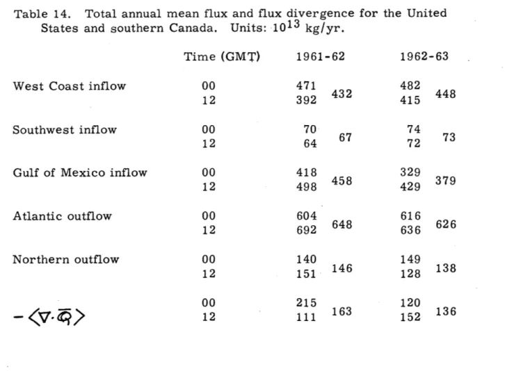
(north of United States- Mexican Border). .. ... ... . .... .. 96 14. Total annual flux and flux divergence for the United States
and southern Canada... 107 15. Annual water balance components-United States and
LIST OF TABLES cont.
16. Annual water balance components-Central Plains and
Eastern Region ... 116
17. Annual water balance components -Western Region ... 117
18. Annual water balance components- Central Plains Region... 121
19. Annual water balance components -Eastern Region... 123
LIST OF FIGURES
Page Figure
Number Number
A-1 1. Distribution of aerological stations used in the investigation.
A-2 2. Vertically integrated mean total water vapor flux vector field, 1958. (From Peixoto and Crisi, 1965). A-3 3. Vertically integrated mean total zonal water vapor
flux, 1958. (From Peixoto and Crisi, 1965). A-4 4. Vertically integrated mean total meridional water
vapor flux, 1958. (From Peixoto and Crisi, 1965). A-5 5. Vertically integrated mean total water vapor flux
vector field, 00 GMT, June-August, 1958.
A-6 6. Divergence of the vertically integrated mean total water vapor flux, 00 GMT, June-August, 1958, computed from mean seasonal flux maps.
A-7 7. Divergence of the vertically integrated mean total water vapor flux, 00 GMT, June-August, 1958, obtained by averaging mean monthly values.
A-8 8. Vertically integrated mean total zonal water vapor flux, 00 GMT; July, 1961.
A-9 9. Vertically integrated mean total zonal water vapor flux, 12 GMT; July, 1961.
A-10
A-11
A-12.
total zonal water vapor
total zonal water vapor
LIST OF FIGURES - cont.
10. Vertically integrated mean flux, 00 GMT; July, 1962. 11. Vertically integrated mean
flux, 12 GMT; July, 1962. 12. Vertically integrated mean
vapor flux, 00 GMT; July, 13. Vertically integrated mean
vapor flux, 12 GMT; July, 14. Vertically integrated mean
vapor flux, 00 GMT; July, 15. Vertically integrated mean
vapor flux, 12 GMT; July, 16. Vertically integrated mean
meridional water
meridional water
meridional water
meridional water
zonal water vapor flux, 00 GMT; January, 1962.
17. Vertically integrated mean total zonal water vapor flux, 00 GMT; January, 1963.
18. Vertically integrated mean total meridional water vapor flux, 00 GMT; January, 1962.
19. Vertically integrated mean total meridional water vapor flux, 00 GMT; January, 1963.
total 1961. total 1961. total 1962. total 1962. total A-13 A-14 A-15 A-16 A-17 A-18 A-19
LIST OF FIGURES - cont.
A-20 20. Difference (12 GMT-00 GMT)/2, of the vertically integrated mean total zonal water vapor flux; June-August, 1961 and 1962.
21. Difference, (12 GMT-00 GMT)/2, of the vertically integrated mean total meridional water vapor flux;
June-August, 1961 and 1962.
22. Differencle, (12 GMT-00 GMT)/2, of the vertically integrated mean total water vapor flux vector; June-August, 1961 and 1962.
23. Difference, (12 GMT-00 GMT)/2, of the vertically integrated mean total zonal water vapor flux;
December-February, 1961-1962 and 1962-1963. 24. Difference, (12 GMT-00 GMT)/2, of the vertically
integrated mean total meridional water vapor flux; December-February, 1961-1962 and 1962-1963. 25. Difference, (12 GMT-00 GMT)/2, of the average
of the wind at the first two standard levels (50 mb intervals) above the ground for July, 1961 and 1962. 26. Difference, (12 GMT-00 GMT)/2, of the average
of the wind at 500 and 550 mb for July, 1961 and 1962. A-21 A-22 A-23 A-24 A-25 A-26
A-28
A-29
A-30
total meridional water, vapor flux, July, 1961 and 1962.
28. Vertical cross section - 30. 0 - 32. 5 0N. Difference
(12 GMT-00 GMT)/2, of mean total meridional water vapor flux, July, 1961 and 1962.
29. Vertical cross section - 30. 0 - 32. 50N. Mean
total meridional water vapor flux, 30-32. 50N, January, 1962 and 1963.
30. Vertical cross section - 47. 5 0N. Mean total meridional water vapor flux, July, 1961 and 1962. 31. Vertical cross section - 47. 50N. Difference,
(12 GMT-00 GMT)/2, of mean total meridional water vapor flux, July, 1961 and 1962.
32. Vertical cross section - 47. 50N. Mean total
meridional water vapor flux, January, 1962 and 1963.
33. Vertical cross section - 800W. Mean total zonal water vapor flux, July, 1961 and 1962.
34. Vertical cross section - 80 W. Difference, (12 GMT-00 GMT)/2, of mean total zonal water vapor flux, July, 1961 and 1962.
A-31
A-32
A-33
A-35
A-36
A-37
A-38
A-39
LIST OF FIGURES - cont.
35. Vertical cross section - 80 0W. Mean total zonal water vapor flux; January, 1962 and 1963.
36. Vertical cross section - west coast. Mean total water vapor influx; July, 1961 and 1962.
37. Vertical cross section - west coast. Difference, (12 GMT-00 GMT)/2, of mean total water vapor influx; July, 1961 and 1962.
38. Vertical cross section - west coast. Mean total water vapor influx; January, 1962 and 1963.
39. Vertical cross section - 1000W. Mean total zonal water vapor flux; January, 1962 and 1963; and July, 1961 and 1962.
40. Hodographs, wind and vapor flux. Stations: 78866 (St. Maarten), 78897 (Guadeloupe), 72201 (Key West). 41. Hodographs, wind and vapor flux. Stations: 80001
(San Andres), 76644 (Merida).
42. Hodographs, vapor flux. Stations: 72253 (San Antonio), 72259 (Brownsville), 72295 (Los Angles), 72493 (Oakland), 72593 (Seattle).
43. Hodographs, wind and vapor flux, Oklahoma City -Tinker AFB.
A-40
A-41
A-42
LIST OF FIGURES - cont.
A-46 44. Hodographs, vapor flux. Stations: 72520 (Pittsburgh), 72562 (North Platte), 72208 (Charleston), 72327
(Nashville), 72235 (Jackson), 72211 (Tampa), 72232 (Burrwood), 72226 (Montgomery), 72274 (Tucson), 72572 (Salt Lake City), 72476 (Grand Junction).
A-47 45. Estimated vertically integrated mean total flux depar-ture vector, 72259 (Ft. Worth), July 1956, 1957, 1958. A-48 46. Mean monthly divergence of the vertically integrated
water vapor flux. May, 1961
A-49 47. Mean monthly divergence of the vertically integrated water vapor flux. June, 1961.
A-50 48. Mean monthly divergence of the vertically integrated water vapor flux. July, 1961.
A-51 49. Mean monthly divergence of the vertically integrated water vapor flux. August, 1961.
A-52 50. Mean monthly divergence of the vertically integrated water vapor flux. September, 1961.
A-53 51. Mean monthly divergence of the vertically integrated water vapor flux. October, 1961.
A-54 52. Mean monthly divergence of the vertically integrated water vapor flux. November, 1961.
A-55
A-56
A-57
A-58
A-59
LIST OF FIGURES - cont.
53. Mean monthly divergence of the vertically water vapor flux. December, 1961.
54. Mean monthly divergence of the vertically water vapor flux. January, 1962.
55. Mean monthly divergence of the vertically water vapor flux. February, 1962.
56. Mean monthly divergence of the vertically
water vapor flux. March, 1962.
57. Mean monthly divergence of the vertically water vapor flux. April, 1962.
58. Mean monthly divergence of the vertically water vapor flux. May, 1962.
59. Mean monthly divergence of the vertically water vapor flux. June, 1962.
60. Mean monthly divergence of the vertically water vapor flux. July, 1962.
61. Mean monthly divergence of the vertically water vapor flux. August, 1962
integrated integrated integrated integrated integrated 62. Mean water
monthly divergence of the vertically vapor flux. September, 1962.
integrated integrated integrated integrated integrated A-60 A-61 A-62 A-63 A-64
A-65
A-66
A-67
A-68
LIST OF FIGURES - cont.
63. Mean monthly divergence of the vertically water vapor flux. October, 1962.
64. Mean monthly divergence of the vertically water vapor flux. November, 1962.
65. Mean monthly divergence of the vertically water vapor flux. December, 1962.
66. Mean monthly divergence of the vertically water vapor flux. January, 1963.
67. Mean monthly divergence of the vertically water vapor flux. February, 1963.
68. Mean monthly divergence of the vertically water vapor flux. March, 1963.
69. Mean monthly divergence of the vertically water vapor flux. April, 1963.
70. Mean seasonal divergence of the vertically integrated
water vapor -flux - Spring (March-May).
71. Mean seasonal divergence of the vertically integrated water vapor flux - Summer (June-August).
72. Mean seasonal divergence of the vertically integrated water vapor flux - Fall (September-November).
integrated integrated integrated integrated integrated integrated integrated A-69 A-70 A-71 A-72 A-73 A-74
LIST OF FIGURES - cont.
A-75 73. Mean seasonal divergence of the vertically integrated water vapor flux - Winter (December-February). A-76 74. Mean annual divergence of the vertically integrated
water vapor flux.
A-77 75. Mean seasonal difference, (12 GMT-00 GMT)/2, of the divergence of the vertically integrated water vapor flux - Summer (June-August).
A-78 76. Mean seasonal difference, (12 GMT-00 GMT)/2, of the divergence of the vertically integrated water vapor flux - Winter (December-February). A-79 77. Regions of water balance computations.
A-81 78. Total net annual flux across selected boundaries. A-82 79. Mean monthly vertically integrated water vapor flux
across various sections of the boundary around the Gulf of Mexico and Caribbean Sea.
A-83 80. Mean monthly vertically integrated water vapor flux across various sections of the boundary around the Gulf of Mexico and Caribbean Sea.
A-84 81. Mean monthly vertically integrated water vapor flux across various sections of the boundary of Northern North America.
LIST OF FIGURES - cont.
A-85 82. Mean monthly vertically integrated water vapor flux across various sections of the boundary of the
United States and Southern Canada, and across the Continental Divide.
A-86 83. Mean monthly vertically integrated water vapor flux across various sections of the boundary of the
United States and Southern Canada, and the net mean monthly inflow to the area.
A-89 84. Water balance - Caribbean Sea
A-91 85. Water balance - Gulf of Mexico and Central American Sea.
A-92 86. Mean monthly difference between precipitation and evapotranspiration - United States, Canada and Alaska; Northern North America.
A-93 87. Water balance - United States - Southern Canada
A-94 88. Mean monthly surface and subsurface storage changes computed from the water vapor balance equation, and estimated by Van Hylckama (1956), for the United States - Southern Canada, and the Eastern Region.
LIST OF FIGURES - cont..
A-97 89. (a) Mean monthly precipitation, and mean monthly estimates of evapotranspiration, obtained from the water vapor balance equation, for the United States-Southern Canada, the Eastern Region, and the
Western and Central Plains Region.
(b) Percentage of total monthly loss due to stream-flow, for the United States and Southern Canada, and the Eastern Region.
A-98 90. Water balance - Western Region
A-99 91. Water balance - Central Plains and Eastern Region A-100 92. Water balance - Central Plains Region
A-101 93. Water balance - Eastern Region
A-102 94. Water balance; Combined Great Lakes - Ohio drainage.
A-105 95. Water Balance - Great Lakes Drainage and Ohio Basin.
A-107 96. Vertical distribution of net water vapor outflow -eastern and western United States.
A-108 97. Analysis of mean annual divergence of the vertically integrated water vapor flux.
LIST OF FIGURES - cont.
A-109 98. Analysis of mean seasonal divergence of the vertically integrated water vapor flux - Spring (March-May). A-110 99. Analysis of mean seasonal divergence of the vertically
integrated water vapor flux - Summer (June-August). A-111 100. Analysis of mean seasonal divergence of the vertically
integrated water vapor flux - Fall (September-November).
A-112 101. Analysis of mean seasonal divergence of the vertically integrated water vapor flux - Winter
(December-February).
A-113 102. Analysis of the mean seasonal difference, (12 GMT-00 GMT)/2, of the divergence of the vertically inte-grated water vapor flux - Summer (June-August). A-114 103. Analysis of the mean seasonal difference, (12
GMT-00 GMT)/2, of the divergence of the vertically inte-grated water vapor flux - Winter (December-February). A-115 104. Mean annual vertically integrated total zonal water
vapor flux, May 1961 - April, 1963.
A-116 105. Mean annual vertically integrated total meridional water vapor flux, May,. 1961 - April, 1963.
LIST OF FIGURES - cont.
A-117 106. Year to year difference in the total vertically inte-grated mean zonal water vapor flux.
A-118 107.. Year to year difference in the total vertically inte-grated mean meridional water vapor flux.
I. INTRODUCTION
Only a portion of the total water substance on this planet actively participates in the physical and biological processes occurring in the atmosphere and the surface layers of the earth. This is the water stored in the oceans, in the atmosphere, and over the land, as surface storage,
s.oil moisture and shallow groundwater. The changes which take place in the total content of these reservoirs undoubtedly proceed at an ex-ceedingly slow rate; consequently, this total water mass can, for most purposes, be considered constant. The principle of continuity, expressed in the form of a balance equation, then becomes the single most useful tool in the study of the processes by which water circulates between and within these reservoirs. In order to best utilize such an
equation, one or more quantities in the equation must be accurately measured, and the remainder evaluated as a residual. It is, therefore, not surprising that the measurement of these quantities has been of
primary concern to hydrologists, and indeed, the modern science of hydrology is often considered to have begun with the 17th century precipitation measurements in the basin of the Seine by the French physicists Perrault and Mariotte (Chow, 1964).
Even at the present time, progress in hydrology is seriously hindered by inadequate measurement of many of the processes involved
in these circulations. Among some of these measurement problems recently discussed by Ackerman (1965) are:
1. Inadequate knowledge of the physical-chemical characteristics of the different soil types (15, 000 in the United States alone), which in turn leads to an inadequate knowledge of soil moisture characteristics.
2. Inadequate information on groundwater storage and movement. 3. Inadequate information on evapotranspiration under various conditions. Ackerman states: "Changes in regional or global supply of atmospheric moisture obtained from land and water surfaces by evapo-transpiration processes are largely unknown... Instruments are in use for measuring evapotranspiration for single site and environment. The effect of changes in environment can be quantified. New instruments or improved techniques for use with conventional instrumentation are needed, however, to quantify the exchange of moisture with the atmos-phere over large areas for which water balance evaluations are required.
General use of the balance equation for the terrestrial branch of the hydrologic cycle has been seriously limited by the existence in the equation of two normally unmeasured quantities, evapotranspiration and change in surface and subsurface storage. Consequently, some additional relationship, involving no additional unknowns, is required in order to solve for these two quantities. The conventional approach
to this problem has centered on attempts to estimate actual evapotrans-piration through the use of standard surface meteorological data. As noted by Thornthwaite and Hare (1965), all these systems contain the same essential elements: (1) a means of computing potential evapotrans-piration, (2) a means of computing actual evapotranspiration and soil moisture, and (3) a system of budgeting soil moisture. Thus, evapo-transpiration is assumed to be a function of potential evapoevapo-transpiration and available soil moisture. Since in these systems potential evapo-transpiration itself is considered a function of meteorological factors, the computed evapotranspiration becomes a function of available soil moisture and meteorological conditions. In the view of many soil scientists, however, the ability of the soil to supply moisture to the surface becomes the dominant factor after the initial drying period. Gardner (1965) states that for much of the period between rains, evapo-ration from the soil is controlled, not by meteorology, but by the ability of soil to transmit moisture. In addition, the question of whether
transpiration decreases as soil moisture decreases, or continues at a constant rate until the permanent wilting percentage is reached, is still considered by many an open question (Thornthwaite and Hare, 1965). The various techniques handle this problem differently.
soil moisture, an estimate must be made of this quantity. The estimated actual storage is kept track of by an accounting technique. Use of
actual measurements of soil moisture are impracticable because of the great variability of such measurements over short distances (Thornth-waite and Hare, 1965). Furthermore, the rate of movement of water to the deeper layers and ultimately to the water table is difficult to evaluate. Recharge (rainfall minus runoff) is handled differently by the various methods; some assume no runoff until the soil moisture deficit is satis-fied (Thornthwaite and Mather, 1955); others make the more realistic assumption that some runoff occurs before the deficiency is satisfied (Kohler and Richards, 1962). As in the case of soil moisture, the run-off used in the accounting procedures is usually computed rather than measured.
The actual value of soil moisture capacity can be measured at a particular site, but this quantity varies from point to point, and its mean value over any given region is essentially unknown. Furthermore, in order to apply these accounting techniques properly over a region, as opposed to a single point, it is not sufficient to know the mean soil moisture capacity; one must also know the distribution of this quantity over the region. Kohler and Richards (1962) attempted to handle this problem by assuming several values of moisture capacity for an area.
The weight which is applied to each value is then determined by cor-relation analysis. These weights depend on the purpose to be served and on the available data. In their case, the weights were determined to yield the best index of storm runoff. Presumably these weights might be different if used for other purposes. In any eve nt, the com-puted soil moisture deficiencies served only as indices in an independent relationship for predicting direct runoff from individual storms.
There is a further problem involved in the use of the terrestrial water balance equation which is sometimes overlooked. This arises from the fact that errors in the measurement of precipitation are not random, but exhibit a negative bias (LaRue and Younkin, 1963). Con-sequently, precipitation measurements will, in most cases, underesti-mate the actual precipitation. This bias, which has been the subject of numerous investigations during the past 80 years, is thoroughly dis-cussed in the comprehensive survey paper of Weiss and Wilson (1957). The error is mainly related to the speed of the wind and the character of the precipitation, and is most serious for the commonly used un-shielded rain gage. Several comparisons have been made between an unshielded gage and a Koschmieder or pit gage, which Weiss and Wilson feel comes closest to giving a useful reference for "true" rain. In most of these tests the unshielded gage underestimated the actual
rain-fall by 5-15% at wind speeds of 4 meters sec 1, 5-30% at 8 meters per second, and 5-50% at 12 meters per second.
Added problems arise in the measurement of snow, and several studies comparing ground measurements of snow with the catch in gages with flexible shields show an average underestimation ranging from 4 to 25% (Weiss and Wilson, 1957). The underestimation is much larger for unshielded gages and gages with rigid shields. General corrections cannot be made for these errors, since the bias is variable and primarily a function of local wind speed.
This bias is accentuated in mountainous areas, where reports are usually sparse and biased toward lower elevations. According to LaRue and Younkin (1963), the paucity of data in the mountainous regions of the United States probably leads to precipitation underestimates of a moderate degree. The lack of adequate precipitation data over large inland lakes, such as the Great Lakes, also creates difficulties.
The average amount by which precipitation is underestimated over North America is, of course, difficult to say, but in the light of the survey of Weiss and Wilson (1957), a figure of 5-10% would not seem unreasonable. This amounts to an average for the United States of about
3. 5 to 7. 5 cm/year, by no means a negligible figure when considering longer term storage changes. Although precipitation measurements
of evapotranspiration, the shortcomings of these measurements must be kept in mind.
Until recent times, the hydrologist has been restricted to measurements involving only the terrestrial branch of the hydrologic cycle. Since the late 1930's, however, an improving network of radio-sonde stations has allowed progressively more detailed measurements of atmospheric water vapor content and flux. These data have given rise to several important studies during the past 15 yearswhich have greatly increased our knowledge of the circulation and distribution of water vapor in the atmosphere.
Because of its high degree of mobility, the atmosphere transports huge quantities of water, even though its mean total water content only approximates that of. the rivers of the edr.th. Thecontinual operation of evaporation and precipitation processes, which are estimated by Budyko (1963) to proceed at an average rate of 100 cm/yr, causes a rapid turn-over in the water content of the atmosphere, and limits the average residence time of atmospheric water to around 10 days.
Over any given region, one finds a source or sink of atmospheric water vapor, the strength of which depends upon the magnitude of the imbalance between evaporation and precipitation at the earth's surface. This must, in the long run, be compensated for by a divergence, either
positive or negative, of the atmospheric vapor flux over the region. Perhaps the most important single finding of the investigations of the past few years, from a hydrologic point of view, was the demonstration by authors such as Starr and Peixoto (1958), Benton and Estoque (1954), Hutchings (1957) and Starr, Peixoto and Crisi (1965) that the vapor flux divergence can be measured accurately enough to give useful estimates of the mean difference between evaporation and precipitation, provided the region considered is not too small and the time period not too short. In these cases, the problems involved in the estimation of evapotrans-piration by empirical techniques can be avoided by using an atmospheric water vapor balance equation (Starr and Peixoto, 1958). Furthermore, for such problems as evaluating the heat balance of the earth-atmosphere, estimating the mean annual runoff from ungaged areas, computing surface and subsurface storage changes over land and, in addition, for many balance problems over ocean areas; it is sufficient to evaluate only the quantity
7-n
; the mean difference between evaporation and precipi-tation. In these cases, the use of the atmospheric water vapor balance equation also avoids the problems arising from the bias in precipitation measurements. There are serious practical problems involved in the use of this approach over smaller regions, but when used over sufficiently large areas, where aerological data is adequate, there is ample reasonto believe that the problems involved are less formidable than those posed by the more conventional empirical techniques.
Extensive atmospheric water vapor flux data has recently become available for the first time. These data were processed as part of a large scale meteorological data processing program, supported by the National Science Foundation under grant: Nos. GP-3657 and GP-820,
and directed by Professor V. P. Starr at M. I. T. These data are, it seems, adequate for a rather detailed study of the water vapor flux and flux divergence over North America, provided certain care is used and certain precautions observed. It was felt that initial studies involving these data should pursue the following goals:
(1) A more detailed description of the atmospheric water vapor flux and flux divergence over the North American sector than has hitherto been possible.
(2) A thorough investigation of the advantages and limitations involved in the use of water vapor flux data in large scale water balance investigations.
(3) A contribution to a better understanding of the overall atmos-pheric and terrestrial water balance of North America.
A study of the water balance of the North American Continent and the neighboring Central American Sea (Caribbean Sea and Gulf of
Mexico), covering the period May 1, 1961 through April 30, 1963, has been made with these goals in mind. This report contains the more important results of that investigation.
II. REVIEW OF PREVIOUS VAPOR FLUX INVESTIGATIONS A considerable number of investigations of atmospheric water vapor flux and flux divergence, on scales ranging from less than 105 km2 to hemispheric, have been made during the past 15 years. Several of these which the author feels to be pertinent to the present investiga-tion will be discussed in this secinvestiga-tion.
Observation of the atmospheric branch of the hydrologic cycle became possible as a result of the rapid expansion of the network of aerological stations just prior to and, in particular, during World War II. Meteorologists and hydrologists were slow in grasping this oppor-tunity and very little use was made of these data until 1950 when Benton, Blackburn, and Snead (1950) used atmospheric flux data in a study of the water balance of the Mississippi Basin.
It had formerly been held by some hydrologists that a large part of the precipitation which fell over continental areas was derived from local sources of evaporation. This misconception arose, according to
Gilman (1964), when the availability of runoff measurements showed that local evaporation amounted to a large percentage of the local
pre-cipitation. This knowledge, combined with an underestimation of the mobility of the atmosphere, led to a gross overemphasis of the direct
conclusions, serious proposals were made to increase precipitation by locally increasing evaporation (Sellers, 1965). Holzman (1937) had
previously recognized the importance of advected moisture to the local water balance and pointed out that most evaporation occurs into drier air enasses, which generally produce little precipitation. The study of Benton, Blackburn and Snead further showed that most water evapo-rated over the Mississippi Basin is carried far outside the basin before falling again as precipitation.
This initial study was followed by a regional study over North America (Benton and Estoque, 1954), which is of considerable
signifi-cance to the present investigation. Using twice daily data at 850, 700 and 500 mb from the rather sparse aerological network in existence over North America in 1949, and using the geostrophic approximation for the winds, Benton and Estoque made estimates of the flux across the continental boundaries, and described the broad scale features of the flux field during 1949. In addition, the computed flux divergence yielded reasonable estimates of average monthly and annual values of E-P for the continent as a whole. These estimates became less re-liable as the size of the area was reduced (Benton, Estoque and Dominitz, 1953).
a small quadrangular area of southern England (9 x 10⁴ km 2) delimited by aerological stations at the four vertices. The investigation included
a statistical analysis of the probable errors in the flux measurements. This analysis is of interest since the vertical resolution in Hutchings' data was similar to that used in the present study, and will be discussed later with respect to data representativeness.
Hutchings (1961) also made a regional study of water vapor
transfer over Australia during the year 1956. The network of Australian stations was roughly comparable to that available to Benton and Estoque over North America in 1949. Once daily data at the surface, 900, 850, 800, 700, 600, 500 and 400 mb levels were used. The study was comp-licated by the frequent occurrence above 850 mb of relative humidities too low to be measured. Nevertheless, the average annual flux diver-gence computed over eastern Australia, assuming the maximum possible mixing ratio in those cases where "motorboating" occurred, was in
excellent agreement with independent estimates of E~P. Mean monthly values were not in particularly good agreement. Lack of agreement during the winter months was probably due in part to errors in the inde-pendent estimate of evapotranspiration. These estimates were obtained by the Thornthwaite method (Thornthwaite and Mather, 1955) which has a tendency to underestimate evaporation during the winter months. One
might suspect that differences during the summer months were due, in part, to diurnal variations in the vapor flux. Such variations were found in the summertime flux over much of North America in the course of the present investigation, and render once daily observations unrepresenta-tive of the mean daily flux.
In a recent study of evaporation over the Baltic Sea, Palm'n (1963) found the average annual flux divergence to be in excellent agree-ment with independent estimates of E-P. These results were based on data from Russian, Finnish, Swedish, Danish, and East German
radio-sondes.
The most extensive studies of the atmospheric branch of the hydrologic cycle, with the aim of finding its relationship to the general circulation of the atmosphere and to the large scale terrestrial water balance, have been conducted as part of the MIT Planetary Circulations Project, under the direction of Professor V. P. Starr. These studies were concerned with average annual or semi-annual conditions. White (1951), in an early study, estimated the water vapor transport across latitude circles from actual wind and humidity reports. This was
followed by a series of investigations based on data from the year 1950. They included an initial study of the poleward flux of water vapor (Starr and White, 1955), followed by a more extensive investigation of the
meridional water vapor flux (Starr, Peixoto and Livadas, 1958). The first study, on a hemispheric basis, of the flux divergence and its rela-tionship to the water balance of the earth was made by Starr and Peixoto (1958). These analyses were later discussed in great detail by Lufkin (1959). The techniques for obtaining the spatial distribution of flux divergence- which are used in the current investigation, were discussed in some detail by Peixoto (1959).
The zonal water vapor flux (Starr and Peixoto, 1960) and the eddy flux (Starr and Peixoto, 1964) have also been studied. The final outcome of the 1950 investigations has been summarized in a monograph (Peixoto, 1958).
Similar studies of the hemispheric water balance (Starr, Peixoto and Crisi, 1965; Peixoto and Crisi, 1965) have recently been completed using the more extensive data available during the IGY year 1958. These data also made possible the first study of atmospheric humidity conditions over the entire African Continent (Peixoto and Obasi, 1965).
III. FORMULATION OF THE BALANCE EQUATIONS The following notation will be used:
= acceleration of gravity
CC = mean radius of the earth
A
longitude= latitude = pressure
= specific humidity
= pressure at the ground
= pressure at which the specific humidity becomes negligibly small = eo4 5. , zonal wind component
V = $ ,meridional wind component
eastward and northward pointing unit vectors, respectively
= total subsurface flow through a unit length of drainage basin boundary
= rate of evapotranspiration
= rate of precipitation
1'O = rate of stream flow from a drainage area
%
= total water storage on and below the surface of the earth per unit horizontal area.of
= net sources of water vapor in a unit atmospheric column ex-tending from
p
to p= time
= number of observations
C
-curve bounding a drainage areat7e
= outward pointing unit normal on curve = time mean( = ( )-- ( = instantaneous departure from time mean
CC'>
=
f()
e
o-.:sgbCal9
=
spatial mean
The -following vertical integrals will be referred to in the course this report:
W
mean precipitable water (gm cm
-2or cm)
vertically integrated mean total 'zonaail water vapor flux (gm (cm sec)~
Tvertically integrated mean total meridiona v c
1 water vapor flux (gm (cm sec).
vertically integrated mean total water vapor flux (gm (cm sec) 1).
The form of the atmospheric water vapor balance equation is essentially that of Starr and Peixoto (1958), and Peixoto and Obasi (1965).
For a column of air, extending from the ground to a pressure one may write the atmospheric water vapor balance equation in the following form:
The atmosphere is assumed to be in hydrostatic equilibrium, and the flux through the upper boundary of the column is ignored, since
is negligible at/4$.
Evapotranspiration from the earth's surface and precipitation falling from the air column constitute the major source and sink of water vapor. The formation (evaporation) of clouds within the column constitutes another possible sink (source), but the use of commonly accepted values for the water content of clouds (aufm Kampe and Weick-mann, 1957; Atlas, 1965) indicates that the flux of water, in liquid and solid form, will rarely average 10 to 20 gm (cm sec)~ for periods of a month or more. This, for example, represents around 1% of the total flux in the regions of persistent wintertime cloudiness along the west coast of North America. Since the flux divergence rather than the flux itself affects the accuracy of the water balance computation, it can be concluded that the transport of water in liquid or solid form may be of some significance in those rather localized regions of per-sistent formation or dissipation of clouds, or for occasional short
time periods, but can be safely ignored on a mean monthly basis for large scale water balance studi,.
Thus
When applied to mean conditions over a given region and time period, Eq. 1 becomes
~
(1:- :11> __ (2)
For annual means, ~ is usually negligible compared with the other terms. For monthly means, however, all terms are often of the same order of magnitude, particularly during the spring and fall.
The vapor flux divergence can be expressed in spherical coor-dinates:
This expression can be conveniently evaluated by finite difference methods to provide the mean divergence within each area defined by 4 grid points. However, when making detailed water balance studies which involve the use of stream flow data, it is usually more convenient to obtain the mean divergence over an irregularly shaped drainage basin. For this purpose, a useful expression for flux divergence may be obtained from Gauss's
Theorem:
e $ -(4)
A second relationship is obtained as a balance equation for the ground branch of the hydrologic cycle. When applied to a particular drainage basin, this balance may be expressed, in its simplest form, as follows:
<RO is the net stream outflow from the basin.
is the mean rate of storage change (surface, soil moisture, and ground-water) over the
basin.
C-C$/7c
c/e
is the net underground flow through the vertical boundaries of the basin. This term will not include ground water flow which discharges into streams within the basin, and contributes only when ground water and surface divides do not coincide. The lack of coincidence of these divides in many limestone and lava regions is well known, and "lost rivers" are commonly encountered in such areas as the Columbia Plateau of the northwestern United States and in the karst areas of Kentucky and Central Europe (Maxey, 1964). Similarly, basins containing large outcrop areas of confined aquifers of broad regional extent may have abnormally low runoff due toprecipi-tation directly entering the aquifer within the basin, or infiltration from streams within the basin. This water is then discharged at downstream points. Typical of this phenomenon are the streams issuing from the mountains onto the alluvial fans of the basin and range province of the Western United States, and the eastward flowing streams of the Black Hills region of North Dakota (Maxey, 1964). These underground ex-changes probably occur on a scale too small to be studied to advantage using the atmospheric water vapor balance equation. Little is known of the larger scale movement of groundwater, which would involve the major aquifer systems, and any interconnections between these systems. Although such exchanges appear to occur in some desert areas (Starr and Peixoto, 1958), they are probably quite small in most regions, and it was felt that attempts to evaluate this quantity over North America would be best deferred to a later time, when data will become available for a period of length sufficient to render surface and soil moisture
storage changes unimportant. Lacking evidence to the contrary, such exchanges were assumed to be small over the large drainage areas investigated, when compared with the seasonal and interannual surface and subsurface storage changes.
Neglect of this term then leaves only two unknowns, =-P,> and, to be evaluated between Eqs. (2) and (5), since< 5T7
can be measured. Solving for surface and subsurface storage change gives:
(6)
Using precipitation measurements, one can also solve for
<5:
These two simple relationships can then be used to evaluate the two unknowns of the terrestrial water balance equation, all other quantities in the equations being measured.
IV. DATA AND PROCEDURES
The-period studied extends from May 1, 1961 through April 30, 1963. 00 GMT meteorological data for the period May 1958 through April 1961 were also available, but were used only for special purposes.
The basic meteorological data were obtained from the MIT GENERAL CIRCULATION LIBRARY and consisted of mean monthly values of the following quantities
N
Separate data were available for 00 GMT and 12 GMT at the surface, 1000 mb and at 50 mb intervalstup to 200 mb for stations over North America and the surrounding area (see Fig. 1). Statistical
esti-mates of g , which are available when the humidity was so low that
"1motorboating" occurred, were treated as actual reports.
and Q) were computed separately for 00 GMT and 12 GMT by applying the trapezoidal rule beginning with the first even 50 mb level above the surface and adding to this the additional
was considered to be the pressure at the ground. Thus it was possible to have reports at pressures high.er than that of the surface in those
cases where the mean monthly .;;face pressure was only slightly
be-low a standard reporting level; these reports were excluded from consider-4ion. Monthly means at levels having less than 10 reports were not
Lsed. Instead the data were considered missing and the value was ob-tained by linear interpolation between the two nearest reporting levels. Stations were considered missing if data did not extend to 700 mb on at least 10 days of the month. Missing values at or above 500 mb were
assumed to be zero if there were no data at higher levels. The total r.a-mber of reports was tabulated for each station for each month in
tie course of the computations.. Examination of these figures indicated that the percentage of missing reports generally ranged between 10% and 20%.
Separate monthly maps were plotted and analyzed for and for each of the 24 months, at both 00 GMT and 12 GMT. In addition, a variety of auxiliary maps were plotted and analyzed in order to obtain additional information on precipitable water, diurnal flux variations, and mean seasonal patterns. Some of these special
charts are included in this report.
difference methods to Eq. 3 (Peixoto, 1959), using as data the values
of q and Q0 on a 2. 50 latitude by 2. 50 longitude grid south of 57. 50N, and on a 5. 00 longitude by 2. 50 latitude grid north of this lati-tude. As before individual computations were made for each month, and separately for the 00 GMT and 12 GMT data.
In order to obtain accurate values of mean divergence for the various irregularly shaped regions considered in the water balance
studies, the net flux across a convenient curve, closely approximating the actual boundary of the basin, was estimated directly from the flux
component maps. It makes little difference for the larger regions whether one approximates a line integral around the basin or estimates
the mean flux divergence directly from the grid point data. On the other hand, it is not always possible to satisfactorily approximate the flux through the boundaries of the smaller regions using only grid point
data. Estimation of the mean flux divergence by planimetering a diver-gence analysis based on grid point data was not considered satisfactory, since the total divergence over an area, as represented by a summation of the flux through the boundary, may not be conserved in the isoline analysis.
Streamflow data were obtained from the Water Supply Papers of the U. S. Geological Survey and Water Resources Papers of the
Canadian Department of Northern Affairs, for an area of 85. 7 x 10⁵ km2 covering almost all of the United States, and much of southern Canada. Immediate coastal regions were notincluded, partly because of the time involved in obtaining runoff from the great number of small coastal streams; and partly due to limitations imposed by the location of the last downstream streamgaging station, which is normally located some distance inland. This had the effect of keeping the boundary of the
drainage area well within the outer ring of aerological stations. Stream-gaging stations used in this study, the areas they gage,, and additional regions of internal drainage are listed in Table 1.
Table 1, Streamgaging stations used in the investigation.
River Station Drainage Area (10 5km 2
Frazier Hope,, B. C. 2. 03
Skagit Mt. Vernon, Wn. 0.08
Cowlitz Castle Rock, Wn. 0. 06
Columbia The Dalles, Ore. 6. 15
Willamette Wilsonville, Ore. 0. 22
Umpqua Elkton, Ore. 0. 10
Rogue Grants Pass, Ore. 0. 06
Klamath Klamath, Ore. 0. 31
Eel Scotia, Calif. 0. 08
San Joaquim Vernalis, Calif. 0. 731
Cosumnes McConnel, Calif. 0. 02
Table 1 cont.
Station Drainage Area (105km2)
Mokelumne Sacramento Colorado Rio Grande Pecos Colorado Brazos Trinity Ne ches Sabine Red Ouachita Mississippi Big Black Pearl Pas cogoula Tombigbee Alabama Escambia Choctawhatchee Apalachicola Suwanee Santilla Altamaha Ogeechee Savannah Edisto Santee Woodbridge, Cali. Sacramento, Calif. Northern In. 'Boudary
U. S. - Mexico
Caballo Dam, N. Mex. Girvin, Tex.
Bay City, Tex. Juliff, Tex. Romayor, Tex. Evadale, Tex. Ruliff, Tex. Alexandria, La. Monroe, La. Vicksburg, Miss. Bovina, Miss. Bogalusa, La.. Merrill, Miss. Leroy, Ala. Clairborne, Ala. Century, Fla. Bruce, Fla. Chattahoochee, Fla. Wilcox, Fla. Atkinson, Ga. Doctortown, Ga. Eden, Ga. Clyo, Ga. Givhans, S. C. Pineville, S. C.
2Includes flow through Yolo Bypass 3
Includes all closed basins entirely within the drainage area. All significant diversions from the basin above the gage are added to the gaged discharge; all diversions into the basin are subtracted.
4Flow estimated from upstream stations and gage height readings 5Includes diversion through Lk. Marion-Moultrie Canal
River 0. 0. 0. 0. 0. 1. 1. 0. 0. 0. 1. 0. 29. 0. 0. 0. 0. 0. 0. 0. 0. 0. 0. 0. 0. 0. 0. 0. 02 672 303 80 77 08 14 44 17 24 75 40 69 07 17 17 504 57 10 11 44 25 07 35 07 26 07 385
Drainage Area (105km2) Peedee Little Peedee Cape Fear Neuse Tar Roanoke James Rappahannock Potomac Susquehanna Delaware Hudson Cone cticut Merrimack Andros coggin St. Francis Richelieu St. Laurence St. Maurice Ottawa Nelson Burntwood Peedee, S.C. Galivants Ferry, S. C. Tarheel, N. C. Kingston, N. C. Tarboro, N. C. Randolph, Va. Cartersville, Va. Fr edi-icksburg, Va. Washington, D. C. Marietta, Pa. Trenton, N. J. Green Island, N. Y. Thompsonville, Conn. Lowell, Mass. Auburn, Me.
Hemming Falls, Que. Fryer's Rapids, Que. Cornwall, Ont. Grand'mere, Que. Grenville, Que. 54047'N, 970561W 55044'N, 97054'W Mississippi Basin Missouri Missouri Mis sissippi Arkansas Ohio
Sioux City, Ia. Hermann, Mo. Alton, Ill.
Little Rock, Ark. Metropolis, Ill. Estimated Additional Internal Drainage Oregon Idaho-Wyoming Utah Nevada California New Mexico
6Estimated from upstream stations
River Station 0.23 0.07 0. 12 0.07 0.06 0.08 0.16 0.04 0.30 0. 67 0.18 0.21 0.25 0.11 0.08 0. 10 0.22 7. 68 0.42 1. 786 10. 09 0.16 8.16 13. 70 4.70 4.10 5.27 0.47 0. 10 1.12 2.52 1.42 0.39
Precipitation data used in this study was obtained from U. S. Weather Bureau Climatological Summaries, the Monthly Report of the Canadian Department of Transport, and a compilation by LaRue and Younkin (1963).
Information on the levels of the Great Lakes was furnished by the Lake Survey of the U. S. Army Corps of Engineers. Computations of evapotranspiration and soil moisture storage for the Ohio Basin, based upon the Thornthwaite method (Thornthwaite and Mather, 1955), were furnished by Mr. Wayne Palmer, of the Environmental Data Service, ESSA. Lake evaporation data (Kohler et al, 1955) was fur-nished by the Hydrologic Research and Development Laboratory of the U. S. Weather Bureau.
Several stations, mostly military operated, converted from the lithium chloride to the carbon humidity element during this two-year period. No significant difference in the measurements obtained from these two elements could be detected in the monthly means; however, the dates of changeover of these stations are listed below.
Table 2. Dates of changeover from lithium chloride to carbon humidity
elements. (Source: National Weather Records Center, Asheville, N. C.) Station
Adak, Alaska Argentia, NFD
Corpus Cristi, Tex. Key West, Fla.
Trinidad, BWI Pt. Arguello, Calif. Guantanamo, Cuba -Kindley AFB, Bermuda
Eglin AFB, Fla. Del Rio AFB, Tex.
Date of Change 9/29/61 1/30/ 61 4/1/61 3/1 /61 5/16/61 1/15/62 2/13/61 Remarks Navy stations
Air Force stations-date of changeover unknown but probably in mid 1961. Del Rio operated by Air Force until 3/3/63, then
operated by the Weather Bureau, who used
lithium chloride element. Oakland, Calif.
Midland, Tex. Intl. Falls, Minn.
Tatoosh, Wn. 4/63 4/63 4/63 4/63 U. S. Weather Bureau
V. REPRESENTATIVENESS OF DATA AND ANALYSES A. Representativeness of the Water Vapor Flux Data
The extent to which the flux data represent the true conditions is determined by (1) how well the data taken at a particular hour, at a particular station, define the actual mean flux at that observing time, and (2) how well the mean of the 00 GMT and 12 GMT observations de-fine the actual mean monthly flux.
The study of Hutchings (1957) previously cited throws some light on these problems, since the resolution of his data (surface and every 50 mb up to 750 mb, then every 100 mb to 350 mb) is similar to that used in the present study. Although not specifically stated, obser-vations were apparently made with the Kew radiosonde. He obtained the following flux vector errors at various levels:
Table 3 Water vapor flux vector errors (from Hutchings, 1957). Units: gm (cm mb sec)-1
Level Systematic Standard vector error
error Total Sampling 950 mb 4.5 +.01 .09 .08 750 mb 3.1 +.07 .07 .06 550 mb 1.5 +.06 .04 .04 350 mb 0.4 +b03 .01 .01
\/ is the mean water vapor flux at the 4 stations during the three month period June-August, 1954. The systematic error was due to humidity errors which were produced by instrumental lag. In this regard, it should be noted that Hutchings assumed no other systematic instrumental errors.
Lag errors in humidity measurements, wind errors, and samp-ling errors arising through the use of the arithmetic mean of two obser-vations a day all contributed to the standard vector error. However, from Table 3 , it is apparent that sampling errors made the major contribution. It will be shown later that diurnal variations in the vapor flux will produce an additional systematic sampling error which often overshadows all others.
The following results were obtained for the vertically integrated transport:
Table 4 . Estimated vertically integrated water vapor flux vector errors (from Hutchings, 1957). Units: gm (cm sec)-1.
Systematic error Standard vector error
+30 16
Sampling errors again make the major contribution to the standard vec-tor error.
The following values were obtained for the flux divergence errors, assuming linear variations between stations:
Table 5 . Estimated vapor flux divergence errors (from Hutchings,
1957). Units: gm (cm 2 mb 3 months)~1.
Level V. Systematic error Standard error
950 mb -0. 302 0 0. 023
750 mb +0. 099 0 0.019
550 mb +0.052 0 0.011
350 mb +0.011 0 0.003
The errors at each level were not serious when compared with the computed values of divergence, even over the relatively small area being investigated. Errors produced by nonlinear flux variations
be-tween stations, which were not included in this estimate, may be more serious, however.
For standard errors of the vertically integrated divergence (including a contribution for nonlinear effects), Hutchings obtained an estimate of 4 g cm-2 for the 3 month period. The magnitude of this error would, of course, decrease as the size of the area increased, provided the same spacing between stations was retained on the bound-ary.
The characteristics of the Kew radiosonde, as to lag and instrumental error, may not be the same as that of the American