MIT Joint Program on the
Science and Policy of Global Change
Analysis of Climate Policy Targets
under Uncertainty
Mort Webster, Andrei P. Sokolov, John M. Reilly, Chris E. Forest, Sergey Paltsev, Adam Schlosser, Chien Wang, David Kicklighter, Marcus Sarofim,
Jerry Melillo, Ronald G. Prinn, and Henry D. Jacoby
Report No. 180 September 2009
The MIT Joint Program on the Science and Policy of Global Change is an organization for research, independent policy analysis, and public education in global environmental change. It seeks to provide leadership in understanding scientific, economic, and ecological aspects of this difficult issue, and combining them into policy assessments that serve the needs of ongoing national and international discussions. To this end, the Program brings together an interdisciplinary group from two established research centers at MIT: the Center for Global Change Science (CGCS) and the Center for Energy and Environmental Policy Research (CEEPR). These two centers bridge many key areas of the needed intellectual work, and additional essential areas are covered by other MIT departments, by collaboration with the Ecosystems Center of the Marine Biology Laboratory (MBL) at Woods Hole, and by short- and long-term visitors to the Program. The Program involves sponsorship and active participation by industry, government, and non-profit organizations.
To inform processes of policy development and implementation, climate change research needs to focus on improving the prediction of those variables that are most relevant to economic, social, and environmental effects. In turn, the greenhouse gas and atmospheric aerosol assumptions underlying climate analysis need to be related to the economic, technological, and political forces that drive emissions, and to the results of international agreements and mitigation. Further, assessments of possible societal and ecosystem impacts, and analysis of mitigation strategies, need to be based on realistic evaluation of the uncertainties of climate science.
This report is one of a series intended to communicate research results and improve public understanding of climate issues, thereby contributing to informed debate about the climate issue, the uncertainties, and the economic and social implications of policy alternatives. Titles in the Report Series to date are listed on the inside back cover.
Henry D. Jacoby and Ronald G. Prinn, Program Co-Directors
For more information, please contact the Joint Program Office
Postal Address: Joint Program on the Science and Policy of Global Change 77 Massachusetts Avenue
MIT E19-411
Cambridge MA 02139-4307 (USA) Location: 400 Main Street, Cambridge
Building E19, Room 411
Massachusetts Institute of Technology Access: Phone: +1(617) 253-7492
Fax: +1(617) 253-9845
E-mail: glo balcha nge@mi t.edu
Web site: htt p://gl obalch ange.m it.edu /
Analysis of Climate Policy Targets under Uncertainty
Mort Webster∗ † #, Andrei P. Sokolov*, John M. Reilly*,Chris E. Forest&, Sergey Paltsev*, Adam Schlosser*, Chien Wang*, David Kicklighter‡, Marcus Sarofim@, Jerry Melillo‡,
Ronald G. Prinn*, Henry D. Jacoby*
Abstract
Although policymaking in response to the climate change is essentially a challenge of risk management, most studies of the relation of emissions targets to desired climate outcomes are either deterministic or subject to a limited representation of the underlying uncertainties. Monte Carlo simulation, applied to the MIT Integrated Global System Model (an integrated economic and earth system model of intermediate complexity), is used to analyze the uncertain outcomes that flow from a set of century-scale emissions targets developed originally for a study by the U.S. Climate Change Science Program. Results are shown for atmospheric concentrations, radiative forcing, sea ice cover and temperature change, along with estimates of the odds of achieving particular target levels, and for the global costs of the associated mitigation policy. Comparison with other studies of climate targets are presented as evidence of the value, in understanding the climate challenge, of more complete analysis of uncertainties in human emissions and climate system response.
Contents
1. INTRODUCTION ... 2
2. ANALYSIS METHODS... 4
2.1 Model Components ... 4
2.2 Monte Carlo Simulation Design... 5
2.2.1 Parameter Distributions ... 6
2.2.2 Sampling Design... 8
2.3 Stabilization Scenarios ... 9
3. RESULTS OF THE ANALYSIS... 12
3.1 Uncertainty in Climate under Stabilization Scenarios... 12
3.1.1 Emissions ... 12
3.1.2 Concentrations... 13
3.1.3 Radiative Forcing ... 18
3.1.4 Temperature Change ... 18
3.1.5 Sea Ice ... 22
3.2 Reduction of the Probability of Exceeding Targets or Critical Levels ... 26
3.3 Uncertainty in the Global Cost of Emissions Mitigation... 29
4. COMPARISON WITH OTHER STUDIES... 31
5. DISCUSSION ... 37
6. REFERENCES ... 40
APPENDIX... 45
∗
Joint Program on the Science and Policy of Global Change, Massachusetts Institute of Technology, Cambridge, MA.
†
Engineering Systems Division, Massachusetts Institute of Technology, Cambridge, MA. #
Corresponding author (email: [email protected]).
&
Dept. of Meteorology, Pennsylvania State University, University Park, PA. ‡
The Ecosystems Center, Marine Biological Laboratory, Woods Hole, MA. @
1. INTRODUCTION
The United Nations Framework Convention on Climate Change (FCCC) states its objective as: “…stabilization of greenhouse gas concentrations in the atmosphere at a level that would prevent dangerous anthropogenic interference with the climate system” (UNFCCC, 1992), and discussion of such a long-term goal is a continuing focus of the Working Group on Long-Term Cooperative Action under the Bali Action Plan (UN FCCC, 2007). This framing of the task has led to a focus on the calculation of the total emissions of CO2 (or of all greenhouse gases stated in CO2-equivalents) that can be
allowed over the century while maintaining a maximum atmospheric concentration. In addition to objectives framed in terms of atmospheric concentrations, the climate goal also has been stated as a maximum increase, from human influence, to be allowed in global average temperature. For example, the European Union has adopted a limit of 2°C above the pre-industrial level, and in 2009 this 2°C target received an endorsement, if not a firm commitment, from the leaders of the G8 nations (G8 Summit, 2009).1 Because of the uncertainty in the temperature change projected to be caused by any path of global emissions, the policy goal is sometimes stated in terms of a maximum increase in radiative forcing by long-lived greenhouse gases, stated in watts per square meter (W/m2). For example, this last approach was taken by a study of stabilization targets undertaken by the U.S. Climate Change Science Program (CCSP) (Clarke et al., 2007), and a set of radiative forcing targets form the basis for construction of scenarios to be used in the IPCC’s 5th Assessment Report (Moss et al., 2007).
Though the climate policy challenge is essentially one of risk management, requiring an understanding of uncertainty, most analyses of the emissions implications of these various policy targets have been deterministic, applying scenarios of emissions and reference (or at best median) values of parameters that represent aspects of the climate system response, and the cost of emissions control. Examples of these types of studies as carried out by governmental bodies include the U.S. CCSP study mentioned above (Clarke et al., 2007) which applied three integrated assessment models to the study of four alternative stabilization levels, and the analysis of the cost of emissions targets in the
IPCC’s 4th Assessment Report (AR4) (Fisher et al., 2007). These efforts provide insight to the nature of the human-climate relationship, but necessarily they fail to represent the effects of uncertainty in emissions, or to reflect the interacting uncertainties in the natural cycles of CO2 and other gases or the response of the climate system to these gases. Where
efforts at uncertainty analysis have been made—e.g., in the IPCC AR4 (Meehl et al., 2007) and studies following on the CCSP report (Wigley et al., 2009)—the results lack consideration of uncertainty in emissions and of some aspects of climate system response (a topic to which we return below).
Here, seeking a more complete understanding of how emissions targets may reduce climate change risk, we quantify the distributions of selected climate and cost outcomes, applying Monte Carlo methods (with Latin Hypercube sampling) to the MIT Integrated Global Systems Model (IGSM), an earth system model of intermediate complexity. This statistical approach cannot fully explore the extreme tails of the distribution of possible outcomes, and there are physical processes (e.g., rapid release of methane clathrates) that are too poorly understood to be included. The method can, however, provide a formal estimate of uncertainty given processes that can be modeled and whose input probability distributions reasonably are constrained. An advantage of the IGSM in this regard is that, in contrast to more complex but less flexible general circulation models, it can span the range of climate responses implied by the climate change observed during the 20th century.
Section 2 describes the methods used in the analysis, including the IGSM, the distributions of its uncertain parameters, the sampling method applied, and the greenhouse gas concentration stabilization policies to be simulated. We present the resulting distributions of model outcomes in Section 3 for the climate response and in Section 4 for the mitigation cost implications. Section 5 compares these results with the outcome of studies with less-complete representations of uncertainty, to show the value of attempts to include a more-complete consideration of human and physical system uncertainties and their interactions. This final section also discusses the implications of the long-term climate targets now under consideration in national discussions and international negotiations.
2. ANALYSIS METHODS 2.1 Model Components
The MIT Integrated Global System Model includes sub-models of the relevant parts of the natural earth system and a model of human activity and emissions. Here we apply Version 2 of the IGSM as described in Sokolov et al. (2005, 2009b). The model includes the following components:
• A model of human activities and emissions, the Emissions Prediction and Policy Analysis Model (Paltsev et al., 2005).
• An atmospheric dynamics, physics and chemistry model (Sokolov and Stone 1998; Wang et al., 1998), which includes a sub-model of urban chemistry (Calbo et al., 1998; Mayer et al., 2000; Prinn et al., 2007).
• A mixed-layer, anomaly-diffusing ocean model [ADOM] (Sokolov et al., 2005; Sokolov et al., 2007), with carbon cycle and sea ice sub-models.
• A land system model (Schlosser et al., 2007) that combines the Terrestrial Ecosystem Model [TEM] (Felzer et al., 2004; Sokolov et al., 2008), a Natural Emissions Model [NEM] (Liu 1996), and the Community Land Model [CLM] (Bonan et al., 2002). Together these components describe the global, terrestrial water, energy, and biogeochemical budgets and terrestrial ecosystem processes that govern them. The climate system component of the IGSM is a fully coupled model which enables the simulation of feedbacks between components. The time steps in the various sub-models range from 10 minutes for atmospheric dynamics to one month for certain terrestrial processes, reflecting differences in the characteristic timescales of the underlying natural phenomena.
The IGSM differs from similar models by its inclusion of significant chemical and biological detail. In particular, natural fluxes of CO2, CH4 and N2O are estimated from
the simulated activities of plants and microbes on land and in the oceans; these vary over the earth’s surface in response to vegetation distribution and simulated variations in light availability as influenced by clouds and aerosols, climate, atmospheric chemistry (CO2
and O3), terrestrial hydrology, and oceanic acidity. The processes governing these natural
organic substrates, ocean acidity and other variables. Global anthropogenic emissions of CO2, CO, NOx, volatile organic compounds (VOCs), black carbon (BC), SOx and other
key species are estimated by a regionally disaggregated model of global economic growth (Paltsev et al., 2005). This procedure allows for treatment over time of a shifting mix and geographical distribution of emissions.
Another feature of the IGSM for uncertainty analysis is its flexibility, allowing it to reproduce the projections of a wide range of 3D Atmosphere-Ocean General Circulation Models (AOGCMs). This aspect of the analysis is accomplished by varying cloud feedback and deep-ocean mixing parameters (Sokolov et al., 2003; Forest et al., 2008). Whereas the climate system response to external forcings, as represented in an AOGCM, is a result of many parametric and structural formulations that are not easily varied, the IGSM can simulate a wide and continuous range of climate response, permitting parametric uncertainty analysis that would not be possible in the larger models.
2.2 Monte Carlo Simulation Design
Monte Carlo simulation is a widely-used set of techniques for characterizing uncertainty in numerical models resulting from uncertainty in model parameters (e.g., Rubenstein and Kroese, 2008). The basic steps in Monte Carlo analysis are: (1) identify uncertain parameters and develop probability distributions for them, (2) sample from the distributions to construct multiple sets of parameter values, and (3) simulate large ensembles of model runs (hundreds or thousands of runs in each ensemble) using the sampled parameter values. The distribution of model outcomes from the ensemble of simulations provides estimates of future uncertainty, conditional on the model structure and the distributions of uncertain parameters.
The results are also conditional on specific assumptions under which future scenarios are constructed. As applied here, the no-policy results assume there are no direct efforts to control emissions of long-lived greenhouse gases. Each of four emissions control levels then creates a different estimate of uncertainty conditioned on achieving that policy target. The ensemble size can also be an issue. With pure random sampling the ensemble size required to obtain an estimate with suitable accuracy can be in the thousands to tens of thousands of model simulations, making this approach infeasible even for models like the IGSM that, although simplified, still require significant computer time. Fortunately,
the size of the required sample can be significantly reduced by applying well-designed sampling strategies. Below, we describe the probability distributions assumed for the model parameters, and the sampling strategy and ensemble size used in our calculations.
2.2.1 Parameter Distributions
The details of the probability distributions developed for each model parameter, as well as the data sources used in constructing each distribution, are documented by Webster et al. (2008a) for the economic model parameters, and by both Forest et al. (2008) and Sokolov et al. (2009b) for the earth system model. Here we briefly summarize these uncertain parameters; their probability distributions are provided in Appendix A.
For the economic (EPPA) model, with its sixteen regions with different characteristics, probability distributions are constructed for over 100 separate socio-economic and
technological parameters. These parameters can be grouped into the following broad categories:
• Elasticities of Substitution • Labor Productivity Growth Rates
• Autonomous Energy Efficiency Improvement (AEEI) • Fossil Fuel Resource Availability
• Population Growth • Urban Pollutant Trends • Future Energy Technologies • Non-CO2 Greenhouse Gas Trends
• Capital Vintaging
The distributions for elasticities of substitution, labor productivity growth rates, AEEI, fossil fuel resources, population growth, and urban air pollutant trends are based on historical data and/or other published studies. The distributions for the cost of future energy technologies, trends of non-CO2 greenhouse gas emissions, and capital vintaging
are based primarily on expert elicitations, documented in Webster et al. (2008a).
Taking advantage of the sensitivity of emissions to each parameter revealed in earlier studies (Webster et al., 2002; Webster et al., 2003), we focus on improving the basis for
emissions per unit of activity, and the elasticities of substitution. An effort was made to base these estimates on observations as opposed to relying on expert elicitation as in our earlier studies. Labor productivity growth rates, which are a primary driver of economic growth in the model, are now based on observed GDP variability over the period 1950-2000. The variability is used to sample future growth rates as a random walk with drift, where the drift is the reference growth path of the EPPA model and the random walk component is sampled for each 5-year period, producing more realistic growth paths where regions experience periods of faster or slower growth. Previous work sampled high or low growth rates that then were applied for the entire 100-year forecast horizon. Future trends in urban pollutants, such as SO2 and NOx, are now based on the stochastic
emissions frontier analysis of 15 countries in Stern (2005, 2006), and so have a stronger empirical foundation. For distributions for elasticities of substitution between different inputs to production (e.g., capital vs. labor, capital/labor bundle vs. energy bundle) we use estimates from published econometric studies.
The probability distributions for uncertain physical parameters in the earth system model are described in Sokolov et al. (2009b). Five uncertain parameters are treated in this study:
• Climate sensitivity
• Mixing of heat into the deep ocean • Aerosol radiative forcing
• CO2 fertilization effect in terrestrial ecosystems
• Precipitation frequency trends as a function of increasing temperature.
The joint distribution of the first three uncertainties – climate sensitivity, ocean heat uptake, and aerosol forcing – is constrained by 20th century observations (Forest et al., 2008). Samples for these three parameters are drawn from their joint distribution in order to capture the interdependence implied by observations. The probability distribution used in this analysis is based on the estimates of the 20th century change in deep-ocean heat content for the 0-3000m layer from Levitus et al. (2005). Other data analyses have been prepared for the upper ocean (0-700m layer) (Domingues et al., 2008; Levitus et al., 2009; Ishii and Kimoto, 2009), which would yield alternative joint distributions. These more recent efforts differ from the earlier Levitus et al. (2005) in the application of bias
corrections to the various ocean temperature records. In addition, the change in ocean heat content below 700m has not been estimated in these more recent data analyses and so assumptions are required about the additional temperature change in the deep ocean. Examples of the sensitivity of future climate projections to the choice of the deep ocean temperature estimates, used to construct input distributions from climate parameters, are given in Sokolov et al. (2009a, b).
We also include here two physical uncertainties not treated by Webster et al. (2003): uncertainty in the CO2 fertilization effect on vegetation productivity, and the change in
the frequency of precipitation as a function of increases in surface temperature. The former affects how much CO2 is removed from the atmosphere by vegetation and
potentially retained in plants and soils. The latter affects emissions of nitrous oxide from soils as those emissions depend on periods of soil saturation. Uncertainty in the carbon uptake by the ocean is not considered as an independent uncertainty but is linked to the uncertainty in the oceanic heat uptake (see Sokolov et al., 2009b for details).
2.2.2 Sampling Design
To limit the ensemble size, we employ stratified sampling (see Rubenstein and Kroese 2008, Ch. 5) and, in particular, the Latin Hypercube method for sampling across multiple parameters (McKay et al., 1979). Numerical experiments demonstrate that, compared with pure random sampling, the outcome distributions converge more quickly to the limiting distributions as sample size increases. We use 400 samples in each ensemble, a sample size that, for Latin Hypercube sampling, has been shown to approximate well the limiting distribution for many nonlinear models2.
As noted previously, there is correlation among some of the input parameters. For the physical climate parameters, correlation is modeled by sampling directly from the joint distribution described in the previous section. For many of the economic parameters, we impose correlation structure on related subsets of parameters (see Webster et al., 2008a
2
For the no policy scenario we tested the adequacy of the ensemble size by comparing sample sizes of 100, 200, 300, 400, 500, and 1000. To do this we performed 20 independent ensembles (drawing different sample sets for each) for each ensemble size, and compared the standard deviation of the estimate of median temperature change to the mean estimate of the standard deviation from the 20 ensembles. The standard deviation of the estimate of the median fell from 0.5% with 100 samples, to 0.2% with 400 samples, and had no appreciable improvement with 500 or 1000 samples. Similarly, the standard
for details). The correlation is imposed during the sampling process using the procedure from Iman and Conover (1982). This method chooses the next subinterval for sampling, without replacement, by imposing the specified rank correlation.
Finally, to estimate the cost of a stabilization target, the simulated macroeconomic consumption in a policy case is subtracted from that in the no-policy case. The procedure involves pairwise comparisons of results for each policy case with that of the no-policy case for each ensemble member, applying identical input values. The same 400 samples are used for all five ensembles, with the only difference among them being the
introduction of different policy constraints. 2.3 Stabilization Scenarios
We base the four stabilization scenarios on those developed, applying the MIT IGSM, for the U.S. Climate Change Science Program (CCSP) Assessment Product 2.1A (Clarke et al., 2007). These cases were designed to provide insight into discussions of climate policy, particularly with regard to the implications of stabilization for emissions
trajectories, energy systems, and mitigation cost. We build on that exercise by performing an uncertainty analysis of each of the CCSP policy constraints. The likelihoods of
different levels of climate change depend on the assumption that these emissions
scenarios are followed over the 100 year simulation horizon, and they are a best estimate of that conditional future based on information we have today as represented by the model structure and input uncertainty.3 Note that the IGSM simulation represents only the potential human perturbation of the climate system, as departures from any natural variability that may be experienced.
The stabilization scenarios in the CCSP exercise were labeled as Levels 1, 2, 3, and 4 (Clarke et al., 2007) and we retain those labels. Each of the emissions paths developed in the MIT component of the CCSP exercise is applied as a vector of constraints on global greenhouse gas emissions beginning in 2015. They are met in each simulated time period and so allow the same cumulative emissions from 2015 to 2100. The quantity that is held
3
More will be learned as time passes policies can be expected to be revised over time as uncertainty is reduced or we learn that median estimates are higher or lower. Nevertheless, analysis of what will happen if we follow a specific path through the horizon remain relevant to the decisions we must make today in the face of existing uncertainty. For studies that examine the implications of hypothetical future resolution of uncertainty see Webster et al. (2008b), Yohe et al. (2004), Kolstad (1996), and Ulph and Ulph (1997).
nearly constant under policy as parameters vary is the cumulative emissions of
greenhouse gases, as weighted by 100-year Global Warming Potentials (GWPs).4 When these emissions levels are propagated through an earth system model with different parameter values, the resulting concentrations will necessarily vary from these targets because earth system feedbacks on concentrations are themselves uncertain and depend on the realized climate.5
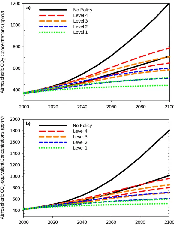
In Table 1, we describe the no-policy and four stabilization scenarios in terms of their cumulative GWP-weighted emissions (denoted as CO2-equivalent (CO2-eq.) emissions)
over 2001-2100, which are 2.3, 3.4, 4.5, and 5.4 trillion (1012 or Tera) metric tons for Levels 1, 2, 3, and 4, respectively. The no-policy scenario has median cumulative emissions of 8.0 trillion metric tons. Table 1 also summarizes the ensemble results for the median levels of
• CO2 concentrations,
• CO2-equivalent concentrations, calculated using radiative forcing due to
long-lived greenhouse gases only (they are listed in Table 2) relative to the pre-industrial level,
• Change in total radiative forcing attributable to the long-lived greenhouse gases and tropospheric ozone and aerosols, and
• Change in global mean surface temperature.
These calculated medians, stated in relation to the 1981-2009 average to be
comparable with results in the IPCC AR4, can help inform policy discussions by giving some idea of the relations between emissions, concentrations and temperature increase.
4
Scenarios where there is low growth in emissions can lead to some ensemble members where emissions are below the constraint level, especially for the Level 4 and Level 3 cases. The variation in GWP-weighted emissions is less than 1%.
5
Both the EPPA and earth system components of the IGSM have been updated since the CCSP study but these emissions scenarios remain of interest in terms of how our current best estimate of the cost of
Table 1. Policy Constraints and Median Values of Key Results from Emissions Scenarios.
Policy
Scenario Cumulative Emissions
Constraints
Median Results for Each Ensemble Decadal Average for 2091-2100 (Changes Relative to 1981-2000 Average) 2001-2100 (Tt CO2-eq)1 CO2 Concen-trations (ppm)2 CO2–eq Concen-trations Long-lived GHGs (ppm)2 Change in Radiative Forcing (W/m2)3 Change in Annual Mean Surface Temperature (°C)3 Level 1 2.3 480 560 2.4 1.6 Level 2 3.4 560 660 3.5 2.3 Level 3 4.5 640 780 4.5 2.9 Level 4 5.4 710 890 5.3 3.4 No-Policy 8.04 870 1330 7.9 5.1
1Calculated using 100-year GWPs as calculated in Ramaswamy, et al. (2001). Includes gases
listed in Table 2.
2 Rounded to nearest 10 ppm.
3 Difference between the average for the decade 2091-2100 and 1981-2000; from
pre-industrial to 1981-2000 the net forcing for the included substances is estimated to be 1.8 W/m2).
4 Ensemble medians.
Table 2. Cumulative ensemble median CO2-equivalent emissions1,2, 2001-2100.
CO2 Emis. (Gt CO2 -eq) CH4 Emis. (Gt CO2 -eq) N2O Emis. (Gt CO2 -eq) HFCs Emis. (Gt CO2 -eq) PFCs Emis. (Gt CO2 -eq) SF6 Emis. (Gt CO2 -eq) Level 1 1400 651 275 3.1 0.4 0.8 Level 2 2330 733 305 4.1 0.4 0.8 Level 3 3340 811 332 4.7 0.4 0.8 Level 4 4120 886 361 5.2 0.4 0.8 No-Policy 5890 1300 531 181 7.3 16.2
1Calculated using 100-year GWPs (Ramaswamy, et al., 2001). 2 Rounded to nearest 3 significant figures.
Table 2 shows the cumulative emissions of each of the long-lived greenhouse gases. The IGSM represents the group of hydrofluorocarbons (HFCs) as HFC-134a and
perfluorocarbons (PFCs) as perfluoromethane (CF4). Other assumptions in constructing the stabilization scenarios are provided in Clarke et al. (2007).
3. RESULTS OF THE ANALYSIS
3.1 Uncertainty in Climate under Stabilization Scenarios
Following Sokolov et al. (2009b), which examined the uncertainty in climate projections in the absence of climate policy, we report results as decadal averages, for example using 2091-2100 to represent the end period of the simulation. The 21st century change is then expressed as the difference from the average for the period 1981-2000. The resulting distributions of outcomes are presented graphically as frequency
distributions of the ensemble results. For each quantity, we choose a bin size such that roughly 50-80 bins are used, and then smooth the results over five-bin intervals. The specific binsize is given in the caption for each figure. The vertical coordinates are normalized so that the area under each distribution integrates to unity.
3.1.1 Emissions
The uncertainty in greenhouse gas emissions under the five scenarios was described in Webster et al. (2008a). Before describing the uncertainty in climate outcomes, we first show the path of the median emissions over time and the 5% and 95% bounds on
emissions for total greenhouse gas emissions in CO2-eq. from that study (Figure 1). The
no-policy case (black lines) has a large uncertainty range, while the policy cases do not exhibit uncertainty, because the emissions constraint is binding – i.e., for the four constraint cases the three lines are on top of one another because of this lack of
uncertainty in total emissions. (In fact, there is some uncertainty, too small to be seen in the figure, in the initial year of the Level 4 and Level 3 scenarios, because under the low-growth ensemble members the constraint is not binding.) There is some uncertainty in the emissions of individual greenhouse gases, such as CO2 or CH4, because of variation
in the relative costs of abatement of the different gases and trading among greenhouse gases is allowed using GWPs (see Webster et al., 2008a).
2000 2020 2040 2060 2080 2100 G lob al G ree nh ou s e Ga s Em is s io n s (B illi on Met ric T ons CO 2 -e q) 0 20 40 60 80 100 120 140 160 180 No Policy Level 4 Level 3 Level 2 Level 1
Figure 1. Global anthropogenic greenhouse gas emissions in CO2-eq in billion metric
tons per year over 2000-2100. Solid lines indicate median emissions, and dashed lines indicate 5% and 95% bounds on emissions. The policy scenario is indicated by the color of lines: no-policy (black), Level 4 (Red), Level 3 (Orange), Level 2 (Blue), and Level 1 (Green).
3.1.2 Concentrations
In Figure 2, we show the uncertainty in concentrations of the main long-lived greenhouse gases averaged for the decade 2091-2100, expressed as frequency
distributions. Naturally, CO2, CH4, and N2O concentrations have a smaller variance in the
stabilization cases than under a no-policy assumption: the policy ensembles implement an absolute constraint on emissions, so almost all emissions uncertainty has been eliminated (see Figure 1). The main source of uncertainty in CO2 concentrations in simulations
under emissions constraint is the rate of carbon uptake by the ocean and terrestrial ecosystems.6
The 95% bounds (0.025 to 0.975 fractile range) of the modeled CO2 concentrations
(Figure 2a) for the no-policy case are 691 – 1138 ppm (a difference of 447 ppm). In
6
As noted above, the IGSM considers uncertainty in carbon uptake by both ocean and terrestrial vegetation. The IGSM accounts for the effect of nitrogen limitation on terrestrial carbon uptake, this significantly reduces both strength of feedback between climate and carbon cycle and uncertainty in this feedback (Sokolov et al., 2008).
simulations applying median no-policy emissions they are 777 and 932 ppm (155 ppm) respectively (which gives an indication of the relative contribution of emissions and earth-system uncertainty). The stabilization policies reduce these concentrations to 95% bounds of 640 – 771 ppm for Level 4 controls (a 131 ppm difference), 580– 696 ppm for Level 3 (a 116 ppm difference), 506 – 597 ppm for Level 2 (a 91 ppm difference), and 442 – 511 ppm for Level 1 (a 69 ppm difference). One implication of these results is that emissions targets intended to achieve specific stabilization goals would need to be
adjusted over time as the uncertainty in the carbon cycle is resolved.
In the CCSP exercise (Clarke et al., 2007) the targets were designed to achieve radiative forcing levels and, given the earth system parameters in the version of the MIT IGSM used there, they also were consistent with ultimate stabilization of CO2 at 750,
650, 550, and 450 ppm. For all but the tightest Level 1 control case, actual stabilization is modeled to occur after the 2100 horizon of the exercise and so concentrations in 2100 as simulated by the IGSM in the CCSP exercise were 677, 614, 526, and 451 ppm in the Level 4 to Level 1 control cases, respectively. The median concentrations for the last decade (2091-2100) in the ensembles developed here are 714, 643, 554, and 477 ppm in the Level 4 to Level 1 in these same cases. The difference in CO2 concentration levels is
due primarily to changes in the parameterization of the carbon uptake by the deep ocean between the two IGSM versions, which leads to lower carbon uptake in the version of the model applied here, as explained in Sokolov et al. (2007).
For CH4 (Figure 2b) and N2O (Figure 2c), there is also still some uncertainty under
the stabilization cases due to the natural emissions of these gases, which depend in turn on temperature and precipitation. Surface temperature influences microbial metabolism, and therefore variations in estimated temperature among ensemble members will result in variations in the estimated rates of methanogenesis and denitrification and the
corresponding natural emissions of CH4 and N2O, respectively. In addition, the intensity
and frequency of precipitation influences the formation of anaerobic zones within the soil where denitrification occurs (Schlosser et al., 2007). Hence, variations in precipitation will alter the extent and duration of these soil anaerobic zones and influence
CO2 Concentrations (ppmv) for (2091-2100) - (1981-2000) 400 600 800 1000 1200 Pro babi lity Den s it y 0.000 0.002 0.004 0.006 0.008 0.010 0.012 0.014 0.016 0.018 No Policy Level 4 Level 3 Level 2 Level 1 a) CH4 Concentrations (ppm) for (2091-2100) - (1981-2000) 2 3 4 5 6 Pr obabi lity Dens ity 0 1 2 3 4 5 6 No Policy Level 4 Level 3 Level 2 Level 1 b) N2O Concentrations (ppb) for (2091-2100) - (1981-2000) 360 380 400 420 440 460 480 500 Pr ob ability De ns ity 0.00 0.02 0.04 0.06 0.08 0.10 0.12 0.14 0.16 No Policy Level 4 Level 3 Level 2 Level 1 c)
Figure 2. Frequency distributions of concentrations averaged for the decade
2091-2100 for (a) CO2, (b) CH4, and (c) N2O. Frequency distributions calculated
using bins of 1.0 ppm/ppb intervals, and smoothed over five bin interval. Horizontal lines show 5% to 95% interval, and vertical line indicates median.
The frequency distribution of the total greenhouse gas concentrations expressed as CO2-eq concentrations – calculated as the CO2 concentrations that would be needed to
produce the same level of radiative forcing, relative to the pre-industrial level (see Huang et al., 2009 for more detail) – is shown in Figure 3. The paths over time of the median and 95% bounds of CO2 are given in Figure 4a. The time paths for CH4 and N2O (not
included here) show similar patterns. Figure 4b shows the same patterns for the CO2-eq
concentrations, considering all the greenhouse gases.
The policies also affect the concentrations of black carbon (BC) and ozone that contribute to radiative forcing (see Appendix B, Tables B3 and B4). Specifically, the concentrations of both species decrease with increasing stringency of the policy.
CO2-equivalent Concentrations (ppmv) for (2091-2100) - (1981-2000)
400 600 800 1000 1200 1400 1600 1800 2000 Pr oba bi lit y Den s ity 0.000 0.002 0.004 0.006 0.008 0.010 0.012 0.014 0.016 0.018 No Policy Level 4 Level 3 Level 2 Level 1
Figure 3. Frequency distributions of concentrations averaged for the decade
2091-2100 for CO2-equivalent for the total of CO2, CH4, N2O, HFCs, PFCs, and SF6.
CO2 equivalence is calculated using instantaneous radiative forcings.
Frequency distributions calculated using bins of 2.0 ppm intervals, and smoothed over five bin interval. Horizontal lines show 5% to 95% interval, and vertical line indicates median.
2000 2020 2040 2060 2080 2100 A tm o sp he ri c C O 2 Con c entr a tion s ( ppm v ) 400 600 800 1000 1200 No Policy Level 4 Level 3 Level 2 Level 1 a) 2000 2020 2040 2060 2080 2100 Atm o spher ic CO 2 -equ iv alent Conc entr a tions ( ppm v ) 400 600 800 1000 1200 1400 1600 1800 2000 No Policy Level 4 Level 3 Level 2 Level 1 b)
Figure 4. 95% probability bounds for decadal averages of (a) CO2 concentrations
3.1.3 Radiative Forcing
The uncertainty in total radiative forcing, which is the sum of the effects of all long-lived greenhouse gases plus troposphere ozone and aerosols, is shown in Figure 5. By the end of this century, radiative forcing has a 95% range of 5.9 – 10.1 W/m2 in the absence of climate policy (7.3 – 8.5 W/m2 due to climate uncertainties only). This range decreases under the stabilization scenarios to 4.0 - 6.0 W/m2 (Level 4), 3.3 – 5.2 W/m2 (Level 3), 2.3 – 4.1 W/m2 (Level 2), and 1.5 – 3.0 W/m2 (Level 1), relative to the average for 1981-2000. The uncertainty in radiative forcing under the stabilization scenarios is due to two factors: (1) as shown above, concentrations vary because of earth system feedbacks on CO2, CH4 and N2O, and (2) there remains emissions uncertainty for sulfates
and carbonaceous aerosols as well as ozone precursors. 3.1.4 Temperature Change
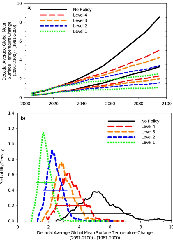
The resulting uncertainty in global mean surface temperature change under each scenario is given in Figure 6. Figure 6a shows the 95% bounds on the decadal average surface temperature change relative to the average for 1981-2000, and Figure 6b shows the frequency distribution of the difference between the average surface temperature for the period 2091-2100 and the average for the period 1981-2000. (Numerical values for selected fractiles are provided in Table B1, Appendix B.) The effect of the stabilization scenarios is to lower the entire distribution of future temperature change, including the mean, median, and all fractiles. The 95% bounds in the no-policy simulations are 3.3 – 8.2oC (3.7 – 7.4oC for climate-only uncertainty). The stabilization scenarios lower this range to 2.3 – 5.0oC (Level 4), 2.0 – 4.3oC (Level 3), 1.6 – 3.4oC (Level 2), and 1.1 – 2.5oC (Level 1).
2000 2020 2040 2060 2080 2100 T o tal Ra diative Fo rc ing ( w /m 2 ) 0 2 4 6 8 10 12 No Policy Level 4 Level 3 Level 2 Level 1 a)
Total Radiative Forcing (w/m2)
0 2 4 6 8 10 12 Pr oba bility Dens ity 0.0 0.2 0.4 0.6 0.8 1.0 1.2 1.4 No Policy Level 4 Level 3 Level 2 Level 1 b)
Figure 5. Total radiative forcing relative to 1981-2000 (greenhouse gases and aerosols) from all emissions for each policy case, shown as (a) 95%
probability bounds over time, and (b) frequency distributions averaged for the
decade 2091-2100. Frequency distributions calculated using bins of 0.1 w/m2
intervals, and smoothed over a five bin interval. Horizontal lines show 5% to 95% interval, and vertical line indicates median.
2000 2020 2040 2060 2080 2100 Dec ada l Aver age Glob al Mean Sur fac e T e m per atur e Chan ge (2091-2100) ( 198 1-20 00) 0 2 4 6 8 10 No Policy Level 4 Level 3 Level 2 Level 1 a)
Decadal Average Global Mean Surface Temperature Change (2091-2100) - (1981-2000) 0 2 4 6 8 10 P rob ab ili ty D e nsi ty 0.0 0.2 0.4 0.6 0.8 1.0 1.2 1.4 No Policy Level 4 Level 3 Level 2 Level 1 b)
Figure 6. Decadal average global mean temperature change shown as (a) 95% bounds over time relative to average for 1981-2000, and (b) frequency distributions of temperature change between the 1981-2000 average and the 2091-2100 average. Frequency distributions calculated using bins of 0.1 degree intervals, and smoothed over a five bin interval. Horizontal lines in b)
An important feature of the results is that the reduction in the tails of the temperature change distributions is greater than in the median. For example, the Level 4 stabilization scenario reduces the median temperature change by the last decade of this century by 1.7oC (from 5.1 to 3.4 oC), but reduces the upper 95% bound by 3.2oC (from 8.2to 5.0oC). In addition to being a larger magnitude reduction, there are reasons to believe that the relationship between temperature increase and damages is non-linear, creating increasing marginal damages with increasing temperature (e.g., Schneider et al., 2007). While many estimates of the benefits of greenhouse gas control focus on reductions in temperature for a reference case that is similar to our median, these results illustrate that even relatively loose constraints on emissions reduce greatly the chance of an extreme temperature increase, which is associated with the greatest damage.
Also, unlike the uncertainty in concentrations and radiative forcing, the uncertainty in temperature change, expressed as percent relative to the median, is only slightly less under the stabilization cases than under the no-policy case. For example, in the decade 2091-2100, the 95% range without policy goes from 40% below the median to 60% above, while the equivalent range under the Level 2 emission target is –33% to +44% of the median. In contrast, the 95% range for CO2-eq concentrations under Level 2 is ±9%
of the median, and the range for radiative forcing is –33% to +18% of the median forcing. Long term goals for climate policy are sometimes identified in terms of temperature targets. As illustrated by these calculations, a radiative forcing or temperature change target does not lead to an unambiguous emissions constraint because, for a given emissions constraint, the resulting temperature changes are still uncertain within this factor of 30 to 40%.
Unclear in such statements regarding temperature targets is whether an emissions constraint set today should be based on the median climate response, or if the goal should be to avoid exceeding a target level of temperature change with a particular level of confidence. The emissions path would need to be much tighter, for example, if the goal was to reduce the probability of exceeding a temperature target to, say, less than one in ten or one in twenty.
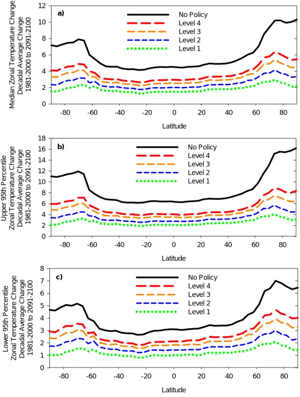
The temperature change resulting from increasing greenhouse gases and other substances will not be uniform with latitude, with the change being greater at high
latitudes and lesser in the tropics (Meehl et al., 2007). Figure 7 shows our estimates of the projected change in the zonal distribution of mean surface air temperature from the 1981-2000 average to the 2091-2100 average under each of the scenarios for the median (Figure 7a), the upper 95% bound (Figure 7b), and the lower 95% bound (Figure 7c). As is the case for global temperature change the reduction due to stabilization in the upper 95% bound is greater than the reduction in the median temperature change.
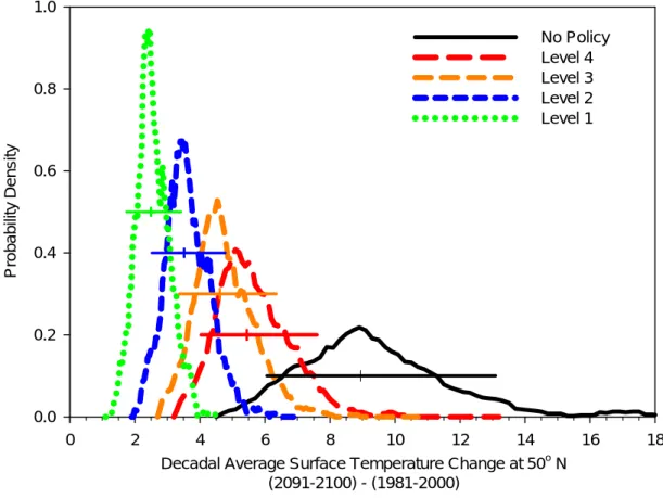
As an example of the impact on high latitude temperature changes, we show the frequency distributions for 60oN–90oN (Figure 8). Numerical values for mean, standard deviation, and selected fractiles are given in Table B3 in Appendix B for a range of zonal bands. As can be seen from these results, climate policies have a larger effect on
temperature changes at high latitudes than on global mean surface warming. The Level 4 policy scenario, for example, would reduce surface temperatures in high latitude regions by between 2 and 7oC relative to the no-policy case or a 40% decrease, compared to a range of 1 to 3oC or a 30% decrease in global mean surface warming.
3.1.5 Sea Ice
Since changes in sea ice are highly correlated with changes in high latitude
temperature, it is not surprising that emissions reductions have a very strong impact on changes in sea ice area in both hemispheres. Figure 9 shows changes in sea ice area (2091-2100 average minus 1981-2000 average) as a fraction of 1981-2000 sea ice area. In the absence of climate policy the median decrease in summer Arctic sea ice is 70% of present day coverage, while even relatively moderate policy (Level 4) decreases the median sea ice loss to 40%. The effect of emission reductions on sea ice changes during local winter is smaller.7
Latitude -80 -60 -40 -20 0 20 40 60 80 Med ian Z onal T em per atur e Change Dec adal Aver age Change 1981 -200 0 to 2091-2100 0 2 4 6 8 10 12 No Policy Level 4 Level 3 Level 2 Level 1 a) Latitude -80 -60 -40 -20 0 20 40 60 80 Upper 95th Per c e n ti le Z onal T em per atur e Change Decadal Av er age Change 1981-2000 to 2091-2100 0 2 4 6 8 10 12 14 16 18 No Policy Level 4 Level 3 Level 2 Level 1 b) Latitude -80 -60 -40 -20 0 20 40 60 80 Low er 95th Per c entil e Zonal T em per atur e Change Decada l A v er age C hange 1981-2000 t o 2091-2100 0 1 2 3 4 5 6 7 8 No Policy Level 4 Level 3 Level 2 Level 1 c)
Figure 7. Zonal mean surface temperature change from the 1981-2000 average to the 2091-2100 average by policy case (a) median zonal temperature change, (b) upper 95th percentile zonal temperature change, and (c) lower 95th percentile zonal mean temperature change.
Decadal Average Surface Temperature Change at 50o N (2091-2100) - (1981-2000) 0 2 4 6 8 10 12 14 16 18 Pr obability Dens ity 0.0 0.2 0.4 0.6 0.8 1.0 No Policy Level 4 Level 3 Level 2 Level 1
Figure 8. Frequency distributions for the decadal average surface temperature
change at 60o-90oN between 1981-2000 and 2091-2100. Frequency
distributions calculated using bins of 0.1 degree intervals, and smoothed over a five bin interval. Horizontal lines show 5% to 95% interval, and vertical line indicates median.
Fractional Change in Sea Ice - September, Northern Hemisphere Change from 1981-2000 average to 2091-2100 Average
-1.0 -0.8 -0.6 -0.4 -0.2 0.0 Pr o b a b ility D e ns ity 0 2 4 6 8 10 12 14 16 18 No Policy Level 4 Level 3 Level 2 Level 1 a)
Fractional Change in Sea Ice - March, Southern Hemisphere Change from 1981-2000 average to 2091-2100 Average
-0.8 -0.6 -0.4 -0.2 0.0 P robab ility Dens ity 0 5 10 15 20 25 30 No Policy Level 4 Level 3 Level 2 Level 1 b)
Figure 9. Changes in sea ice area (2091-2100 relative to 1981-2000) as a fraction of 1981-2000 coverage for (a) Northern Hemisphere in September, and (b) Southern Hemisphere in March. Frequency distributions calculated using bins of 0.0025 intervals, and smoothed over a five bin interval. Horizontal lines show 5% to 95% interval, and vertical line indicates median.
3.2 Reduction of the Probability of Exceeding Targets or Critical Levels
An important feature of uncertainty results is the ability to demonstrate that emissions control brings greater reduction in the tails of distributions than the median. And because there is evidence that marginal damages are increasing with the degree of climate change, targets are frequently stated in terms of conditions “not to be exceeded” as noted in the Introduction. Thus a useful way to represent the results in Section 3.1 is in terms of the probability of achieving various targets. Three examples are shown here. Global mean surface temperature is often used as an indicator of climate change for this purpose, as it relates to impacts on human and natural systems. Temperatures in the high latitudes are important for the stability of the large ice sheets of Greenland and Antarctica as well as the stability of permafrost regions. And reduction of sea ice extent, along with polar temperatures, is an important input to study of the fate of the deep ocean circulations.
We show the probability of exceeding several illustrative targets for global mean temperature change (from 1981-2000 to 2091-2100) under the policy scenarios in Figure 10. For a very low temperature change target such as 2°C, the Level 4 and Level 3 cases decrease the probability only slightly. The Level 1 case reduces the probability of
exceeding 2°C to about 25% or a 1 in 4 odds. In contrast, higher temperature change targets, such as 4°C, exhibit convexity; Levels 4 or 3 reduce the probability of
exceedence significantly, with little incremental gain from more stringent reductions in the Level 2 and Level 1 cases. The numerical values in the form of odds are given in Table C1 in Appendix C.8
8
Regarding the precision of the odds of low probability outcomes, the Latin Hypercube sample of 400 model runs cannot resolve likelihoods of outcomes of less than 1 in 400, and the actual precision is less than that due to the random nature of the draw for any one sample. Also, as noted earlier, there are hard to quantify aspects of climate response and economic activity, such as how ocean temperatures were used to constrain climate parameters, how to represent economic growth, and processes that are not well characterized and thus not represented in our (or any) modeling system (such as the behavior or large ice sheets, or possible large scale biogeochemical feedbacks from Arctic systems). Methods that could address some of these issues include; a larger sample size or an importance sampling design
(Rubenstein and Kroese, 2008) or a meta-uncertainty analysis weighting estimates derived from different data sets. Complementary methods, such as expert elicitation may be of some use for incorporating highly speculative processes because they can more readily integrate different lines of
REF Level 4 Level 3 Level 2 Level 1 Pro bab ility of E x ce edin g Il lustrativ e Glo bal M ea n S urf a c e Tem pe ratu re T arget (%) 0 20 40 60 80 100 2 Degrees C 3 Degrees C 4 Degrees C 5 Degrees C 6 Degrees C
Figure 10. Change in the probability of exceeding illustrative targets for global mean surface temperature change, as measured by the change between the
average for 1981-2000 and the average for 2091-2100. Lines indicate the change in probability under different policy cases for exceeding a given
target: 2oC (green dotted line), 3oC (blue dashed line), 4oC (orange dashed
line), 5oC (red dashed line), and 6oC (black solid line).
As an illustration of how the probability of exceeding temperature targets at high latitudes change, we calculate the average temperature change between 60oN and 90oN. In Figure 11, we show the probability for each ensemble that the temperature change for this latitude band over the next century will exceed 3, 4, 5, 6, 7, and 8oC. For example, the odds that the average surface temperature change for 60oN-90oN exceeds 5oC are 98 in 100 in the no-climate policy ensemble, and decrease to 9 in 20 under Level 4, 2 in 10 under Level 3, 1 in 100 under Level 2, and there are no simulations above 5oC under Level 1 (Table C3).
Besides the likelihood of achieving particular policy targets with an emissions limit, this form of presentation may also be useful in illustrating the effects on specific components of the climate system. One candidate is the change in sea ice at the end of summer (September for the Northern Hemisphere, March for the Southern Hemisphere).
REF Level 4 Level 3 Level 2 Level 1 Pr obabi lity o f E x c e eding Illu str ativ e T ar g et f o r A v e rag e Sur fac e T e m p er atu re C hang e 60 N-90N ( % ) 0 20 40 60 80 100 3 Degrees C 4 Degrees C 5 Degrees C 6 Degrees C 7 Degrees C 8 Degrees C
Figure 11. Change in the probability of exceeding illustrative targets for average
surface temperature change at 60oN to 90oN, as measured by the change
between the average for 1981-2000 and the average for 2091-2100. Lines indicate the change in probability under different policy cases for exceeding a
given target: 3oC (green dotted line), 4oC (blue dashed line), 5oC (orange
dashed line), 6oC (red dashed line), 7oC (black solid line), and 8oC (brown
REF Level 4 Level 3 Level 2 Level 1 Pr obab ility ( % ) of Ex ceeding Ill u str a tiv e T a rg et f o r Chan g e in Sea Ic e Ex ten t fr om 1 981-2000 Av e ra g e Septe m be r, N or th er n H emisphe re 0 20 40 60 80 100 ΔSea Ice < -20% ΔSea Ice < -30% ΔSea Ice < -40% ΔSea Ice < -50% ΔSea Ice < -60%
Figure 12. Change in the probability of exceeding illustrative targets for changes in sea ice extent in September in the Northern Hemisphere relative to the average for 1981-2000. Lines indicate the change in probability under different policy cases for exceeding a given target: 20% decrease (green dotted line), 30% decrease (blue dashed line), 40% decrease (orange dashed line), 50% decrease (red dashed line), and 60% decrease (black solid line).
Figure 12 shows the probability from this analysis that the decrease in September northern hemisphere sea ice cover from the 1981-2000 average to the 2091-2100 average exceeds 20%, 30%, 40%, 50%, and 60%. For example, the odds of a decrease in sea ice cover of more than 40% is 97 in 100 without climate policy, and falls to 2 in 5, 15 in 100, 1 in 100, and less than 1 in 400 under Levels 4, 3, 2, and 1, respectively (Table C4). Similar odds are given in Table C5 for the Southern Hemisphere in March.
3.3 Uncertainty in the Global Cost of Emissions Mitigation
The CCSP study of stabilization scenarios (Clarke et al., 2007) yielded, for each participating model, a set of single estimates of the cost of achieving the atmospheric targets, but of course the cost of achieving any global emissions target also is uncertain. Monetized, global estimates of the cost of emissions mitigation over the century are subject to many qualifications, discussed by Clarke et al. (2007), but nonetheless we extend our illustration of the risk management framing of climate policy decisions by
No Poli cy Lev el 4 Leve l 3 Lev el 2 Lev el 1 Gl o bal Consumpti o n L o ss (% ) 0 1 2 3 4 95% Probability Bounds 50% Probability Bounds Median a) No Poli cy Leve l 4 Level 3 Leve l 2 Leve l 1 G lo bal C o n s umption L o ss (% ) 0 2 4 6 8 10 12 14 95% Probability Bounds 50% Probability Bounds Median b) No Po licy Leve l 4 Leve l 3 Leve l 2 Leve l 1 G loba l Co nsu m pt io n Los s ( % ) 0 5 10 15 20 25 95% Probability Bounds 50% Probability Bounds Median c)
Figure 13. Median, 50%, and 95% probability bounds of consumption loss (%) relative to no-policy case for the years (a) 2020, (b) 2060, and (c) 2100. Solid black line indicates median, dark grey shading indicates 50% probability interval, and light grey shading indicates 95% probability interval.
reproducing the results for uncertainty in the costs of emissions reductions as computed by Webster et al. (2008a). As in Webster et al. (2008a) and Clarke et al. (2007), we use the loss in global aggregate consumption as the measure of cost. Figure 13 shows the uncertainty in the costs of abatement in 2020, 2050, and 2100 for the five scenarios. In
contrast to the probability of exceeding climate targets, which falls as the emissions cap is tightened; the uncertainty in costs grows as the emissions cap is decreased.
4. COMPARISONS WITH OTHER STUDIES
Formal uncertainty analysis of the type shown here is computationally demanding, and as a result is infrequently conducted. Sometimes, however, assessments interpret the range of outcomes across models as a proxy for the uncertainty range, or include uncertainty in some but not all of the relevant processes. What is gained by the more complete representation of uncertainty in this paper can be shown in a comparison of our results with examples of other approaches.
One example is the CCSP study from which we drew the greenhouse gas constraints used in the IGSM calculations performed for that study and adopted here. The IGSM was one of three models used in the study; the other two were the MERGE and
MiniCAM models (Clarke et al., 2007). These models have very different structures, and in the CCSP study no effort was made to calibrate them to common assumptions about economic growth, technology costs or other aspects of economic and emissions behavior. As a result of these inter-model differences, there was in the CCSP study, as in other multi-model assessments, the potential to take the difference in results among the model results as a measure of uncertainty—this despite warnings by the CCSP report’s authors that such a procedure was inappropriate.
Figure 14 shows why this warning was warranted and illustrates the limitations of multi-model assessments as a basis for forming judgments about uncertainty. For the reference and each constraint, Level 1 through Level 4, the figure repeats the probability distributions of CO2 concentrations in 2091-2100 from Figure 2a. Also shown in Figure
14 are five horizontal lines with black circles indicating the range of point estimates from the different models in Clarke et al. (2007) for the particular policy scenario. For the IGSM, the reference case used in the CCSP study is below the median in the current calculations, in part because of model changes since the earlier analysis was done. But what is important for this comparison is the magnitude in estimated uncertainty between the two approaches. In all cases, the range of model point estimates is much narrower
CO2 Concentrations (ppmv) in 2100 400 600 800 1000 1200 Pr oba bi lity Dens ity 0.000 0.002 0.004 0.006 0.008 0.010 0.012 0.014 0.016 0.018 No Policy Level 4 Level 3 Level 2 Level 1
Figure 14. Frequency distributions, and medians and 95% bounds, of CO2
concentrations averaged for the decade 2091-2100. Frequency distributions calculated using bins of 1.0 ppm/ppb intervals, and smoothed over five bin interval. Horizontal lines with single vertical line in center indicate 5%-95% range and vertical mark indicates median from this study. Horizontal lines with three circles indicate range of reported results from Clarke et al. (2007), and circles indicate the point estimates from the three models.
than the uncertainty range—indeed, less than 50% of the range calculated for the IGSM alone.9
Taking another step toward uncertainty analysis, Wigley et al. (2009) used these same CCSP emissions scenarios to conduct an analysis similar to the current study, but
incomplete in its representation of uncertainty. The authors propagate the emissions scenarios developed by the three models in Clark et al. (2007) through the MAGICC model, a single simplified gas-cycle/climate model, to assess the ranges of results for concentrations, radiative forcing, temperature change and sea level rise associated with the uncertainty in anthropogenic emissions.
9
Climate related uncertainty in temperature change was estimated using just the emissions scenario from the MiniCAM model, with uncertainty in system response represented just by the lower and upper bounds from the IPCC’s 90% confidence interval for climate sensitivity: 1.5oC and 6.0oC. It is then asserted that, because contributions from uncertainties in other climate parameters are much smaller, the resulting ranges of temperature change should represent the 90% confidence interval on temperature change (conditional, of course, on a given emissions projection). The 90% ranges in this study are 3.5oC to 7.4oC for No Policy and 0.7oC to 2.4oC for Level 1 cases, with median warming of 2.8oC and 1.4oC, respectively.
The 90% range for the no-policy case in our study that can be compared with the Wigley et al. (2009) estimate is the range for a single (median) emissions projection as estimated by Sokolov et al. (2009b) which is 3.8oC to 7.0oC, whereas our range for Level 1 is 1.2oC to 2.4oC.10
Our median warming is larger in both cases, with values of 5.1oC and 1.8oC,
respectively. In the no-policy case, the difference is partly due to higher emissions; for example, Wigley et al. (2009) calculate a 3.5oC warming for EPPA no-policy emissions. Because the median value of climate sensitivity in our simulations (2.9 oC) is very close to the median value used by Wigley et al. (2009), the remainder of the differences between the two studies is the result of differences in the heat uptake by the ocean and radiative forcing. While our absolute 90% range for temperature changes in the no-policy case is slightly wider than the one in Wigley et al. (2009), our relative ranges are
narrower for both scenarios: from 26% below the median to 360% above the median for no-policy and from -31% to 39% for Level 1. The smaller uncertainty ranges in our projections of surface warming is explained by the fact that we use a joint probability distribution of climate sensitivity, aerosol forcing, and ocean heat uptake that is
constrained by the climate change observed during 20th century. As discussed by Forest et al. (2008), 20th century climate changes rule out low values of climate sensitivity (our 90% range is 2.0oC to 5.0oC) and also impose correlation between climate sensitivity, the rate of ocean heat uptake, and the strength of aerosol forcing.
10
The comparison of results is not exact since Wigley et al. (2009) show the difference between values at 2100 and 2000 rather than between 2091-2100 and 1981-2000 averages.
0 2 4 6 8 10 12 Cum ulative Pr o bab ility 0.0 0.2 0.4 0.6 0.8 1.0 No Policy Level 4 Level 3 Level 2 Level 1
Figure 15. Cumulative probability distributions of global mean temperature change from decadal average for 1861-1870 (preindustrial) to the decadal average for 2091-2100.
As a consequence of the above differences, the likelihood of meeting a temperature target of 2oC above preindustrial (adding 0.7oC to the calculated results to include the warming since pre-industrial) under the Level 1 policy differs between these two studies. Wigley et al. (2009) estimate a 50% probability whereas the relatively small change in the lower tail of the distribution in our analysis lowers this probability to only 20% (Figure 15).
Another example of partial uncertainty analysis is the IPCC Fourth Assessment Report (AR4), which presented probability bounds on some of its projections, conditional on each of several different SRES emission scenarios (Nakicenovic et al., 2000). These scenarios together with the 90% range of results from the IPCC AR4 AOGCMs (where available), and the distribution of temperature change from our simulations, are shown in Figure 16. This comparison suggests that the IPCC projections significantly
underestimate the risks of climate change in the absence of an emissions constraint. The significantly larger chance of greater climate change in this study than in the IPCC is due
emissions for the IPCC SRES scenarios with the emissions used in this study can be found in Prinn et al. (2008) and Webster et al. (2008a). As noted by Webster et al. (2008a) only the A1FI and A2 scenarios fall within the uncertainty range for our no-policy case. Given our analysis, the other SRES scenarios are unlikely absent the influence of climate policy. It has been widely observed that the SRES scenarios,
originally constructed in the mid-1990s, underestimated emissions trends of the last 10 to 15 years and are well-below observed emissions today (Canadell et al., 2007; Pielke et al., 2008). IPCC B1 IPCC A1T IPC C B 2 IPC C A 1B IPCC A2 IPC C A 1FI No Polic y Lev el 4 Lev el 3 Leve l 2 Lev el 1 Gl oba l M ean S ur fa c e T em p erature C hang e ( o C) Di ff erence B etw een 19 81-200 0 an d 20 91-210 0 0 2 4 6 8 10 12
Figure 16. Comparison of global mean temperature change (from 1981-2000 to 2091-2100) uncertainty ranges for IPCC SRES scenarios (Meehl et al., 2007) and from this analysis. The grey bars for IPCC results indicate the “likely” range (between 66% and 90% probability), and solid black line indicates the 5-95% range of AOGCM results (only provided for B1, A1B, and A2). Results from this analysis are shown as box plots, where box indicates the 50% range and center line is median, outer whiskers indicate the 10-90% range, and the dots indicate the 5-95% range.
With regard to the climate response, Prinn et al. (2008) compared the IGSM forced by the anthropogenic emissions for SRES scenarios and showed significantly higher surface warming than that produced by the IPCC AR4 AOGCMs. The difference is explained by a few factors. Due to a different treatment of carbon-nitrogen interactions, the terrestrial carbon uptake simulated by the IGSM is smaller than the one simulated by the carbon-cycle model used by the IPCC. The IGSM also takes into account climate change related increases in the natural emissions of methane and N2O. As a result, greenhouse gas
concentrations simulated by the IGSM for a given SRES scenario are higher than the concentrations for the same scenario used to force the AOGCMs in the simulations described in IPCC AR4 (Meehl et al, 2007). As can be seen from results presented by Prinn et al. (2008), changes in surface air temperature (SAT) in the IGSM simulations with median no-policy, Level 4 and Level 2 emissions are very close to surface warming obtained in simulations in which the IGSM was forced by the IPCC concentrations for A1FI, A1B and B1 scenarios, respectively. In addition, the rates of oceanic heat uptake for almost all of the AR4 AOGCMs lie in the upper half of the range implied from the Levitus et al. (2005) estimates of the 20th century changes in the heat content of the deep ocean. As shown by Sokolov et al. (2009a), surface warming projections obtained in the IGSM simulations with climate input parameter distributions based on the Domingues et al. (2008) estimates of changes in deep ocean heat content are closer to the results of the IPCC AR4 AOGCMs.
As can be seen from Figure 16, the “likely”11, ranges given by the IPCC AR4 are significantly wider than both 90% ranges in the simulations with the MIT IGSM and the 90% probability ranges based on the simulations with the AR4 AOGCMs. Meehl et al. (2007) construct a “likely” range for temperature change of 40% below the best estimate to 60% above the best estimate, with the best estimate being a mean value of surface warming projected by the AOGCMs. The long upper tail of the “likely” range is explained, in part, by the possibility of a strong positive feedback between climate and the carbon cycle (Knutti et al., 2008). As mentioned above, taking into account the nitrogen limitation on terrestrial carbon uptake makes this feedback much weaker (Sokolov et al., 2008). However, as noted earlier, ocean data and other aspects of the
analysis, if varied produce a different range, and so a meta-analysis across these different data sources and approaches would yield still greater uncertainty. A detailed comparison between our no-policy case and the IPCC AR4 results is given by Sokolov et al. (2009).
Currently, a new round of scenario analyses is underway that would provide for a common basis for climate model runs in the IPCC AR5. Guidance for those scenarios is provided in Moss et al. (2008). Four Representative Concentration Pathways (RCPs) are being prepared, which are described as: “one high pathway for which radiative forcing reaches > 8.5 W/m2 by 2100 and continues to rise for some amount of time; two intermediate "stabilization pathways" in which radiative forcing is stabilized at approximately 6 W/m2 and 4.5 W/m2 after 2100; and one pathway where radiative forcing peaks at approximately 3 W/m2 before 2100 and then declines.” The radiative forcing increase in the RCPs is specified from the preindustrial level. All RCP pathways reflect cases in the published literature with the first three based on the CCSP scenarios. Thus, not coincidentally, the analysis reported here is approximately consistent with the RCP scenarios. In particular, the median of our no-policy case (see Table 1) — when corrected to a change from pre-industrial by the addition of an estimated of 1.8 W/m2 increase12 — is consistent with the “high and rising” RCP, while our Level 2 (3.5 + 1.8 = 5.3 W/m2 above preindustrial by 2100) and Level 1 (2.4 + 1.8 = 4.2 W/m2) are roughly consistent with achieving stabilization sometime after 2100 at 6.0 and 4.5 W/m2
respectively.13 The analysis presented here thus may provide an assessment of uncertainty to complement the scenario analysis being developed for the IPCC AR-5.
5. DISCUSSION
Deciding a response to the climate threat is a challenge of risk management, where choices about emissions mitigation must be made in the face of a cascade of
uncertainties: the emissions if no action is taken (and thus the cost of any level of control), the response of the climate system to various levels of control, and the social
12
Our estimate of 1.8 W/m2 is derived from the GISS model (Hansen et al., 1988), the radiation code from
which is used in the MIT IGSM. The IPCC estimates the change in radiative forcing from preindustrial
to present to be 1.6 W/m2, based on their estimates of the forcing from individual GHGs (Forster et al.,
2007). 13
We do not have a case comparable to the 3 W/m2 as that was not in the CCSP scenario design, and