Analysis of fuel behavior in the spark ignition engine start-up process

ANALYSIS OF FUEL BEHAVIOR IN THE

SPARK IGNITION ENGINE START-UP PROCESS

by

Michael J. Sampson

Submitted to the

Department of Mechanical Engineering in Partial Fulfillment of the Requirements

for the Degrees of

MASTER OF SCIENCE IN MECHANICAL ENGINEERING and

BACHELOR OF SCIENCE IN MECHANICAL ENGINEERING at the

MASSACHUSETTS INSTITUTE OF TECHNOLOGY May 1994

© 1994 Massachusetts Institute of Technology All rights reserved

Signature of Author

Department of•ecdanical Engineering May 6, 1994 Certified by

Jdhn B. Heywood

Professor, Department of Mechanical Engineering

...-'- .-- -Thesis Supervisor

/

Accepted by

Ain A. Sonin C airman, Department Graduate Committee

Eng

MASSACHUJS'.i I NSIT

Or .F l

_ I_

ANALYSIS OF FUEL BEHAVIOR IN THE SPARK IGNITION ENGINE START-UP PROCESS

by Michael J. Sampson

Submitted to the Department of Mechanical Engineering on May 6, 1994 in partial fulfillment of the requirements for the degrees of

Master of Science in Mechanical Engineering and Bachelor of Science in Mechanical Engineering

ABSTRACT

An analysis method for the characterization of fuel behavior during spark ignition engine start-up has been developed and applied to several sets of start-up data. The data sets were acquired from modem production vehicles during room temperature engine start-up. Two different engines, two control schemes, and two engine temperatures were investigated. The fuel accounting used was a cycle-by-cycle mass balance for the fuel, where the amount of fuel injected was compared with the amount burned or exhausted as unburned hydrocarbons. The difference was measured as "fuel unaccounted for". The calculation for the amount of fuel burned used an energy release analysis of the cylinder pressure data. The results include an overview of starting behavior and a fuel accounting

for each data set. Differences between start-up strategies are discussed and areas for improvement are identified.

Overall, starting occurred quickly, with combustion quality, manifold pressure and engine speed beginning to stabilize by the seventh cycle, on average. To facilitate this rapid starting at cold engine conditions, approximately five times the amount of fuel required for a stoichiometric mixture is injected during the first one or two cycles. A large portion of this fuel, equivalent to nearly ten injections at stoichiometric idle conditions, remains "unaccounted for" after ten cycles of this analysis. Close to 10% of the fuel injected during the initial overfueling that is "unaccounted for" at first, shows up later in underfueled cycles as burned fuel or as hydrocarbon emissions. Similar trends occurred with both engines, temperatures, and start-up strategies; although, during warm engine start-up conditions the overfueling is only 130% of stoichiometric, and the mass "unaccounted for" after ten cycles represents only one injection at idle. The most successful start-up strategies that were analyzed injected close to the stoichiometric requirement for each cycle after the initial overfueling. The stoichiometric requirement for a particular cycle is directly proportional to the manifold pressure at a given

temperature and therefore it is recommended that methods for using manifold pressure in start-up strategies be investigated.

Thesis Advisor:

John B. Heywood

"And to love life through labour is to be intimate with life's inmost secret." K.G.

ACKNOWLEDGMENTS

During my six year visit at M.I.T. there have been many people who have made my life and my education (is there a difference?) more enjoyable. This is my opportunity to thank them:

My parents - without their love and support none of this would have happened. The Tech Sports Car Club / M.I.T. Racing Team - perhaps the most important and certainly the most enjoyable aspect of my M.I.T. experience.

Professor John Heywood - for the guidance, advice, insights and introductions, and for teaching me the methods associated with good research and engineering.

Professor Chris Atkeson - for the support (monetary and otherwise), enthusiasm, and willingness to take a risk; your energy is contagious - hope you're enjoying the warm weather.

Ed VanDuyne - a mentor, an inspiration, a racer, a friend - thanks.

Doug Foster - for all the work with the model and the "lawnmower from hell", thanks for saving me from South Carolina; for the racing and the friendship. Hi Sandy!

Paul, my blood brother - words don't seem appropriate; I'll shake your hand next time I see you.

Soon, Adam, Sean, Mike, Moon, Faris, Steve, Jim, Jabo, Goose and anyone who ever went to a "MechE social" for all the good times here. Pam, Michelle and Derek -old friends are the best.

Doug Hamrin - for the help with FORTRAN, the proofreading, the beer and for helping me keep things in perspective this past year.

The folks at the Sloan Lab and at Adrenaline, especially Paul, Bob, Joan and Brian.

Doug and Hillary for the proofreading; Tina for the data entry; Bob Warshow for Figure 1.3.

Bill Kryska, Tom Rolewicz, Steve Smith and John Hoard from Ford's Advanced Powertrain Division - for the data used in this project and for the advice and feedback.

TABLE OF CONTENTS ABSTRACT ... 3 ACKNOWLEDGMENTS ... 5 LIST OF FIGURES ... 7 LIST OF TABLES ... 8 CHAPTER 1 - INTRODUCTION 1.1 Motivatio n .. ... 9 1.2 Background ... 10

1.2.1 Air & Fuel Behavior ... 10

1.2.2 Engine Control Systems ... 11

1.3 Objective ... 13

CHAPTER 2 - EXPERIMENTAL OVERVIEW 2.1 Vehicles and Engines ... 16

2.2 Data Acquisition ... 16

2.3 Test Conditions and Procedure ... 17

2.4 Overview of Start-up Performance ... 18

CHAPTER 3 - FUEL AND AIR MODELS 3.1 Fuel Injector Mapping ... 25

3.2 Energy Release Analysis ... 25

3.2.1 Overview ... 25

3.2.2 Mixture Model ... 26

3.2.3 Other Assumptions ... 29

3.2.4 Outputs ... 31

3.2.5 Sensitivities ... 32

3.3 Feedgas Hydrocarbon Measurement...34

CHAPTER 4 - FUEL ACCOUNTING 4.1 Fuel Injected ... 41

4.2 Fuel Burned ... 41

4.3 Hydrocarbon Output ... 42

4.4 Fuel Unaccounted For ... 43

CHAPTER 5 - RESULTS AND DISCUSSION 5.1 Simultaneous Injection...50

5.2 Sequential Injection ... 53

5.3 Warm Start... .55

5.4 Discussion ... 57

5.5 Summary and Conclusions ... 58

REFERENCES ... 73

LIST OF FIGURES

Figure 1.1 Liquid Fuel in the Intake Manifold and Port Runners ... 14

Figure 1.2 Diagram of a Typical Intake Port ... 14

Figure 1.3 Schematic of a Typical Control System ... 15

Figure 1.4 Visualization of a Spark Timing "Map" ... 15

Figure 2.1 Behavior of Manifold Pressure, Speed and Cylinder Pressure During Start-up ... 21

Figure 2.2 Fuel Injected vs. Fuel Required for a Stoichiometric Mixture During Start-up ... 22

Figure 2.3 Normalized Cylinder Work Output During Start-up ...23

Figure 2.4 Overview of Engine Behavior During Start-up ... 24

Figure 3.1 Fuel Injector Calibration Curves ... 36

Figure 3.2 Example Output from the Burn Rate Program ... 37

Figure 3.3 Effect of the Mass In Estimate on the Fuel Mass Burned Result ...38

Figure 3.4 Effect of the Stoichiometry Estimate on the Mass Fraction Burned Result ... 38

Figure 3.5 Effect of the Stoichiometry Estimate on the Fuel Mass Burned

Result

...

39

Figure 3.6 A Sample Feedgas Hydrocarbon Measurement ...40

Figure 4.1 A Sample Injector Pulsewidth Measurement ... 45

Figure 4.2 Mass of Fuel Injected Per Cylinder During Start-up ...46

Figure 4.3 Window for the Estimation of Engine Speed and Manifold

Pressure ...

47

Figure 4.4 A Sample Feedgas Hydrocarbon Trace ... 48

Figure 4.5 Sample Result of Fuel Accounting ... 49

Figure 4.6 Sample Cumulative Fuel Unaccounted For Result ...49

Figure 5.1 Mass of Fuel Injected during the Simultaneous Start-up ...61

Figure 5.2 Fuel Injected vs. Fuel Requirement - Simultaneous Start-up ...61

Figure 5.3 Speed, Manifold Pressure, Hydrocarbon Output, and Cylinder Pressure traces - Simultaneous Start-up ... 62

Figure 5.4 Normalized Work Output - Simultaneous Start-up ...63

Figure 5.5 COVimep - Simultaneous Start-up ... 63

Figure 5.6 Fuel Accounting Result for One Cylinder of the Simultaneous Start-up ... 64

Figure 5.7 Cumulative Mass of Fuel Unaccounted For - Simultaneous Start-up ... 64

Figure 5.8 Mass of Fuel Injected during the Sequential Start-up ...65

Figure 5.9 Fuel Injected vs. Fuel Requirement - Sequential Start-up ...65

Figure 5.10 Speed, Manifold Pressure, Hydrocarbon Output, and Cylinder Pressure traces - Sequential Start-up ... 66

Figure 5.11 Normalized Work Output - Sequential Start-up ...67

Figure 5.12 COVimep - Sequential Start-up ... 67

Figure 5.13 Fuel Accounting Result for One Cylinder of the Sequential

Start-up

...

68

Figure 5.14 Figure Figure Figure Figure Figure Figure 5.15 5.16 5.17 5.18 5.19 5.20 Figure 5.21

Cumulative Mass of Fuel Unaccounted For - Sequential

Start-up ... 68

Mass of Fuel Injected during the Warm Start-up ... 69

Fuel Injected vs. Fuel Requirement - Warm Start-up ...69

Speed, Manifold Pressure, Hydrocarbon Output, and Cylinder Pressure traces - Warm Start-up ... 70

Normalized Work Output - Warm Start-up ... 71

COVimep - Warm Start-up ... 71

Fuel Accounting Result for One Cylinder of the Warm Start-up .. .... ... 72

Cumulative Mass of Fuel Unaccounted For - Warm Start-up ... 7... 72

Engine Parameters ... 16

Experimental Test Matrix ... 18

Sensitivity of Burn Rate Predictions to Key Inputs ... 32 LIST OF TABLES

Table 2.1 Table 2.2 Table 3.1

CHAPTER 1- INTRODUCTION

1.1 Motivation

For many years the government and the public have been demanding an increase in fuel efficiency and reduction in pollutant emissions from the spark ignition engine. Recent Clean Air Act amendments have placed very strict limits on the amount of hydrocarbon fuel that can be emitted. This work has been motivated by the belief that the understanding of fuel behavior during engine start-up, which is an extreme transient process under open loop control, will aid in the development of systems and strategies that improve emissions and efficiency.

During gasoline engine starting, a large amount of fuel is injected into the intake port to get the engine started as quickly as possible. A large fraction of this fuel ends up as a liquid film, or 'puddle', on the port walls, on the intake valve, and in the cylinder. This 'puddle' also exists during many normal, warmed-up engine operating conditions. Figure 1.1 (page 14) indicates operating conditions where liquid fuel was observed in an engine with central fuel induction. Engines with port injection frequently have fuel puddles due to the short amount of time allowed for vaporization. If the size and transient behavior of this puddle were better understood then the overfueling, and resulting hydrocarbon emissions, that commonly occur during transients might be reduced. Additionally, when liquid fuel from this puddle enters the cylinder, it reduces the effectiveness of the oil. Over a time this dilution contributes to the breakdown of the entire oil supply. Liquid fuel in the cylinder also increases pollutant emissions.

To compensate for an incomplete knowledge of the fuel behavior, a complicated control system incorporating air measurement, fuel metering, engine and exhaust sensing, microprocessor feedforward and feedback control has been developed by automobile manufacturers. However, even with current feedback and lead/lag compensators it is not

always possible to obtain the desired performance. Compensation schemes that predict air and fuel behavior can significantly improve the performance of these systems, but further advancements need to be made with these prediction techniques in order to meet stricter demands.[Hendricks] Because of the dynamics involved and the previous work in the field, fuel behavior is generally considered more difficult to estimate than airflow.

The start-up process has recently become the focus for efforts aimed at reducing emissions. Approximately 75% of the CO and hydrocarbon emissions occur in the first minutes of engine operation during the Federal emissions test cycle. [Almkvist] This is due to the time required to warm-up the exhaust catalyst and the oxygen and airflow sensors. With the improvement of feedback control systems and exhaust gas catalysts, the total amount of hydrocarbons that are emitted is being reduced. However, since these systems require time to warm up, an increasing proportion of the emissions are occurring at engine starting and warm-up. In order to meet the most stringent upcoming standards, it will be necessary to improve hydrocarbon output during the start, run-up and early warm-up phases of engine operation. At the same time, customer expectations require a rapid start under all operating conditions. It is a great challenge to meet these stringent and conflicting demands.

1.2 BACKGROUND

1.2.1 Air & Fuel Behavior

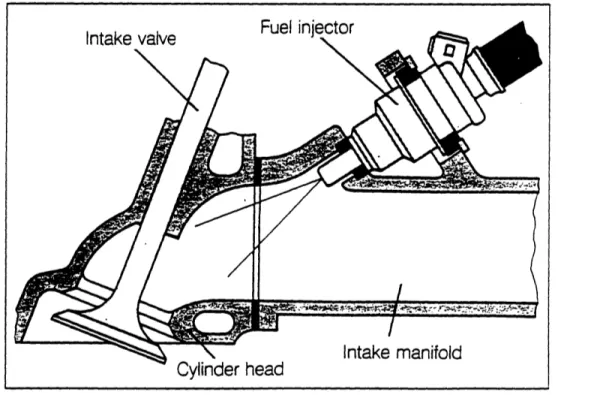
The generation of a combustible mixture within the cylinder, and specifically at the spark plug, is governed to a large part by the fuel behavior within the port. The fuel metering in most modern engines is accomplished with injectors located at the entrance to each intake port, with the fuel spray aimed at the back of the intake valve. Figure 1.2

injected during the exhaust stroke when the intake valve is closed. The injectors atomize the fuel into small droplets (-100m) that either evaporate or form a film on the port walls and intake valve. Vaporization of this film puddle within the port depends on factors such as engine speed, port and valve temperatures, and inlet pressure. As the intake valve opens there is often hot exhaust back flow from the cylinder that further enhances fuel vaporization. This flow then reverses and the mixture of exhaust gasses, fresh air and evaporated fuel flow into the cylinder. A portion of any liquid fuel remaining in the port may also be drawn in before the valve closes.

During transient engine operation the air and fuel behavior is rapidly altered. Fuel evaporation, puddle behavior and liquid fuel flows are unsteady. Changing manifold pressures and air flows cause difficulty in determining the proper amount of fuel to inject. The cycle-to-cycle timing of injection is also a consideration because of the difference in the dynamic time constants of the air and fuel flows. A less than

optimal mixture is inducted into the cylinder if there is not proper compensation for these effects.

At engine start-up, the air transients are extreme and the fuel evaporation is poor. According to [Shayler], at 16 deg. C, only 25-30% of the injected fuel is in vapor form inside the cylinder during the first few cycles of cranking. Current starting strategies compensate for this by injecting approximately five times the required fuel during the first cycle or first two cycles at room temperature.

1.2.2 Engine Control Systems

To meet the conflicting demands of higher performance, lower emissions and greater efficiency, microcontroller based feedback systems have been developed. A typical system is shown in Figure 1.3.

The controller attempts to optimize combustion by sending signals to the fuel injector drivers and spark coils based on inputs from the various sensors. The readings

from the sensors reference predetermined look-up table 'maps'. Typically the spark timing map is based on the engine speed and air flow. Figure 1.4 is a visualization of a spark timing map. In many systems this base map is altered due to conditions such as knocking and the amount of exhaust gas recirculation. The fuel injection map is also based on air flow and engine speed. During most operating modes the signal from the exhaust gas oxygen sensor is used as a feedback signal to trim the fuel injection command to produce the required air/fuel ratio for the exhaust catalyst. The fuel command is also commonly altered by engine temperature, sudden large throttle

transients and battery voltage. Several engine operating modes, notably engine start-up and idle, are usually treated as distinct modes of operation that are not controlled from the 'base maps', but have their own strategies.

During engine start-up, fuel injection and spark timing are controlled using an open loop strategy. The exhaust oxygen sensor and most air flow sensors require several seconds to reach operating temperature before their signals can be used as control inputs. The fuel injection command is based primarily on temperature. After several very large injections (how large and how many depending on how cold the engine is) fuel is cut back. The subsequent level of enrichment is based on time and temperature. Usually, during warmed-up engine operation, each injector is fired at the same relative point in the cycle for its respective cylinder (sequential injection). An older alternative is for the injectors to open at the same point in time (simultaneous injection). However, for the first cycle or two during start-up the injectors do not have the ability to fire sequentially due to the nature of the shaft encoder that provides speed and position information. Therefore, the injectors are commonly fired simultaneously until the encoder can provide absolute position information. The injections then gradually adjust to their proper

sequential timing over the next several cycles. At start the spark timing is fixed at a retarded value, based on engine speed, until a certain engine speed is reached and the

1.3 OBJECTIVE

The objective of this research is to characterize engine start-up behavior, focusing on the fuel transport. Several sets of start-up data have been analyzed, incorporating runs with two different engines and both room temperature soaked and warm-engine room temperature starts. The results include: 1) an overview of behavior during starting, and 2) a fuel 'accounting' for each run based on fuel injected, engine-out hydrocarbon measurements and estimates of fuel burned using an energy release analysis of the cylinder pressure traces.

This thesis summarizes the analysis method and explains the results of the preliminary data sets. An overview of the experimental setup and procedure is given, including engine specifications, measurements, and operating conditions. The fuel accounting method is explained in detail, with descriptions of the air, fuel and energy release models. Results for several starts are presented and discussed. Suggestions are made for future work as well as possible improvements to the starting strategy and control methodology.

0 1000 2000 3000 4000 Engine speed, rev/min Engine speed, rev/min

(a) (b)

Figure 1.1 Regions of engine operation with liquid fuel in (a)

port runner, for centrally inducted fuel. [Heywood]

intake manifold and (b)

Figure 1.2 Diagram of a typical inlet port in a modem engine displaying

and orientation of the fuel injector. [Probst]

the position m -imcj E .m to C me a .F -U _=. CE 400 300 200 100 0 5000 Cylinder nead _ __ v 30

i

I

Figure 1.3 Schematic of a Typical Control System. Signals from the sensors are used by the electronic engine controller to determine values for the control of the actuators.

Igniticn advance

-_, 'seer

Figure 1.4 Visualization of a Spark Timing "Map" showing the dependence of the

spark ignition timing signal on engine speed and load. [Probst]

CHAPTER 2 EXPERIMENTAL OVERVIEW

2.1 VEHICLES AND ENGINES

All of the data used in this research was provided by the Advanced Control Systems Group of Ford's Advanced Powertrain Division. Two different vehicles were tested: a 1991 Thunderbird with a 3.8 liter V6 engine, and a 1992 Lincoln Town Car with a 4.6 liter V8. The tests were conducted in the Allen Park test facility where the cars were on chassis dynamometers. A description of the engine parameters is given in Table 2.1. These engines and vehicles were production units except for alterations to the starting strategy as noted in Section 2.3.

Table 2.1 ENGINE PARAMETERS

4.6L V8 3.8L V6

Bore [mm] 90.2 96.8

Stroke [mm] 90.0 86.0

Con. Rod Length [mm] 150.7 150.2

Compression Ratio 9.02 9.00

Valves/Cylinder 2 2

Valve Events: IVO [BTC] 12 18

IVC [ABC] 64 56

EVO [BBC] 63 70

EVC [ATC] 21 20

Firing Order 1-3-7-2-6-5-4-8 1-4-2-5-3-6

Approx. vehicle mileage 2,000 8,000

2.2 DATA ACQUISITION

The engines were thoroughly instrumented during the start-up testing. Data acquisition was performed using a high speed digital sampling system to capture the first thirty cycles of engine operation. For each cylinder the fuel injector pulse and

information was also collected. A fast response, flame ionization hydrocarbon detector (FID) was used to sample the exhaust. The sample point was located in the head pipe before the catalytic converter and after the union of the manifold pipes. Other recorded quantities include signals used by the engine controller to represent different modes of operation (such as crank or run-up) and a clock channel that allows the data to be displayed in a time representation.

2.3 TEST CONDITIONS AND PROCEDURE

The tests represent the first portion of the Environmental Protection Agency's Federal Test Procedure emissions driving cycle. The test conditions reproduced an 'in-service, typical' start as closely as possible. Each start-up test was conducted at room temperature and atmospheric pressure (approximately 1 bar and 230C) with the vehicles in park on a chassis dynamometer. The engine was either at room temperature or close to operating temperature, depending on the test. Both cars had low mileage and were running on indolene. The battery was always fully charged. Starting was initiated by a driver in the vehicle turning the ignition key, and the data acquisition was triggered automatically by the turning of the crankshaft.

The tests include starts with two different engines, two different control schemes, and two different engine temperature conditions. The test matrix is outlined in Table 2.2. The two vehicles/engines are described above in Section 2.1. The 'Cold' temperature condition refers to the engine at room temperature. This was achieved by allowing the car to sit for an extended period, or by force cooling with external heat exchangers and fans. The 'Hot' start was done after the engine had reached operating temperature. The car was shut down, and started again before any significant cooling had occurred.

The two starting strategies differed in the manner that fuel injection was synchronized at the early stage of start. The 'simultaneous' scheme is representative of the production strategy, where all the injectors are fired simultaneously until the control

unit can determine the absolute position of the engine. At that point each injection is gradually shifted, over the next few cycles, to the correct relative location for its cylinder. The 'sequential' injection strategy is a method where additional position information is provided to the controller. This allows each injector to start delivering fuel at the same relative point for its cylinder from the very beginning of start. There are also other, more subtle changes in the start-up strategy, such as the exact point where the controller changes modes. These changes do not effect the objective of this study, and are not included in this analysis.

Table 2.2 EXPERIMENTAL TEST MATRIX

Test Engine Strategy Temperature

1 V6 Sequential Cold

2 V8 Simultaneous Cold

3 V8 Sequential Cold

4 V8 Simultaneous Hot

2.4 OVERVIEW OF START-UP PERFORMANCE

A close look at the starting process allows a better understanding of the tradeoffs and difficulties involved. Identifying trends in engine parameters can aid in discovering particular phases of the process and may help with the development of control strategies. This description will also make it easier to understand the analysis explained later.

Figure 2.1 (page 21) shows several of the outputs for a typical start. The intake manifold pressure is initially at atmospheric pressure, and starts to decrease after the first complete cycle. The pressure falls rapidly as the engine utilizes the air in the manifold while the throttle remains nearly closed. By the sixth cycle the pressure is

approximately one half of atmospheric pressure and the rate of pressure drop has decreased. By 12 cycles the pressure is very close to the minimum value, and after

approximately 20 cycles the minimum of 1/3 atmosphere has been reached and the pressure starts to increase slightly.

The crankshaft speed increases drastically during the first several cycles. The transition from the cranking speed of 150 RPM occurs before the end of the first engine cycle as one of the cylinders late in the sequence fires on its first pass. Within three cycles the speed has reached 1000 RPM. After this point the acceleration is less pronounced, and the maximum speed of 1500 RPM occurs at 8 cycles. The speed then decreases almost linearly until it levels out at approximately 900 RPM.

The in-cylinder pressure for cylinder number two is shown as a reference point. The first cycle is a non-firing cycle, as shown by a low maximum pressure relative to the manifold pressure. The second cycle is clearly a firing with a high intake pressure. The subsequent cycles have a peak pressure that follows the same trend as the manifold pressure.

Figure 2.2 shows the amount of fuel injected and the amount of fuel required for a chemically optimal (stoichiometric) air/fuel ratio during a typical room temperature start. The strategy consists of three distinct phases: the initial, very large injections where there is substantial excess fuel, the following injections that are below the stoichiometric level, and the subsequent injections that are close to the amount of fuel required for that cycle. Two different cylinders are displayed, showing that occasionally a cylinder will only get one very large injection pulse. For the data provided, the

overwhelming majority of cylinders (greater than 80%) received two large injections. Figure 2.3 presents the relative work output for each cycle of each cylinder normalized by the manifold pressure during the intake process for each cycle. Work is measured as indicated mean effective pressure (IMEP), which is the work output divided

by cylinder volume. Dividing again by manifold pressure gives insight into the stability of the combustion process, since the manifold pressure is proportional to the mass of charge in the cylinder. Since all of the cylinders show a negative work output, the first

cycle is a cranking cycle. During the next cycles, only a fraction of the cylinders have a significant output. By the seventh cycle the balance between the cylinders has improved, and the variation remains almost constant. It can also be noted that the work output scales well with the manifold pressure, since the outputs are all of the same magnitude.

Figure 2.4 gives an overview of several engine parameters based on data from numerous starts. The process can be divided up into several distinct phases: Cranking, Unstable Combustion, Combustion Stabilization, and Steady Idle. The cranking phase commonly lasts for less than two cycles before a significant firing of cylinders. Unstable combustion occurs in the following three to five cycles, as the manifold pressure rapidly drops and the fuel and air flows rapidly change. Combustion stabilization starts as the engine reaches peak RPM, the manifold pressure begins to level out, and each cylinder begins to receive a similar charge of air and fuel. Approximately 15 to 20 cycles after the first firing, the engine settles into a fairly steady idling with minor changes in manifold pressure, speed, and cylinder work output.

I ' OK I ' 5K 10K Degrees l lT l I I I I I I I I I I I I 15K 20K 25K

Figure 2.1 Behavior of Manifold Pressure, Speed and Cylinder Pressure verses

crankshaft degrees during engine Start-up. Peak cylinder pressure approximately

follows the trends of manifold pressure. Engine speed rises rapidly during the first eight cycles. 14- 12- 10o-8-p S -6-: 4- 2- 0-3 400] .50] I I 25Oxj 100-3_I I 150: 3 o-i . I Speed -1400 --1200 -1000 .-800 R P M d Pressure ler Pressure -5K -600 r -400 --200 3-0 30K - -.V 1 1 . 1 1 1 l. - 1 .l l . . - . . . - 'l

0.180.16 0.14 -0.12 0 I 0.1-' 0.08 0.06- 0.04-0.02 n-I _ I

IL IL

Z,

IL

Figure 2.2 Mass of fuel injected vs. mass of fuel required for a stoichiometric mixture

with the inducted air. Examples of the first five cycles of the 3.8L V6 start-up showing that some cylinders receive two injections of overfueling and some have only one.

* Fuel Injected O Fuel Required for a

Stoichiometric Mixture

* Fuel Injected

[l Fuel Required for a Stoichiometric Mixture rA U.Z

i,

1,

_L

1,

1,

12 10 8 a_m

E6

Figure 2.3 Normalized work output for each individual cylinder in sequence during

P mnifold Atmospheric

Peak cylinder pressure decreases to approx. half of WOT fire

Many cycles are late burning

Crank Rapid acceleration (aprox. 200 rpm/cycle)

R450 -almost constant

pH ai ce~cto (po.20rncce

Peak RPM Occurs

Peak IMEP IMEP decrease from 2/3 peak to 1/3 peak

occurs

per-cycle StDev IMEP has leveled of f by this point

Slight decrease

Nearly steady (within 200rpm)

nearly steady at 1/3 original

peak

Key on Manifold Pressure Stabilizng rank Unstable Combustion

Combustion Stabilizlng

-2 _{0 2 6}

CycLes

per

CyLinder

Figure 2.4 Overview of engine behavior during Start-up compiled from observations

of many raw data sets. Average behavior is displayed.

P cylinder non large I (VOT) firing freT FIRST FIRE I RPM IMEP 8 ₁₀ 12 Nearly steady

CHAPTER 3 - FUEL AND AIR MODELS

The primary objective of this work is the determination of the fuel behavior during start-up. This determination is performed for each cycle of each cylinder, and involves the calculation of the amount of fuel that is injected, the amount that is burned, and the amount that leaves the exhaust manifold as unburned hydrocarbons. This chapter describes the models, assumptions and estimated accuracy of these calculations.

3.1 FUEL INJECTOR MAPPING

The quantity of fuel injected into an engine can be accurately determined by recording the signal to the injector solenoid. The pulse width time of this signal is proportional to the time that the injector is open. The injectors are calibrated by measuring fuel flow for a given pulse width and battery voltage. Figure 3.1 (page 36) presents an injector calibration graph.

From the multiple calibrations developed for an injector, one curve was produced which was used in the determination of fuel input. This was done by assuming the battery voltage was 13.5 V. Since the calibration data only included points for average length injections, and there are several very long duration injections during starting (5

times average), the calibration curve was assumed to extrapolate linearly. Changing battery voltages, variations between injectors, and the resolution of the data acquisition results in an estimated uncertainty of 5%.

3.2 ENERGY RELEASE ANALYSIS 3.2.1 OVERVIEW

A single-zone burn-rate model based on in-cylinder pressure was used to determine the amount of fuel oxidized during the combustion process. This model,

developed by Cheung at the Sloan Automotive Lab at M.I.T., uses a heat release approach based on the First Law of Thermodynamics [Cheung]. The model inputs include: the cylinder pressure data, the engine geometry, the amount of charge inducted each cycle, a fuel/air ratio and several thermodynamic parameters. The program first calculates the fraction of residual and the resulting mass of fuel inducted. The central part of the program then calculates the mass fraction burned and burning rate profiles. The outputs consist of the burn profiles, as well as statistics for these parameters and for the pressure data. To determine the mass of fuel burned during each cycle, the maximum mass fraction burned value is multiplied by the estimate for the mass of fuel inducted that cycle. The assumptions for the model inputs, and the uncertainty of the outputs, are discussed in the following sections.

3.2.2 MIXTURE MODEL

The primary inputs for the fuel burn model are the in-cylinder pressure and the makeup of the fuel/air charge in the cylinder. The pressure is acquired from the engine, but the constituents of the charge must be estimated. During steady state, warmed-up engine operation the air mass-flow sensor can determine the air inducted per cycle, and the fuel mass can be calculated from the exhaust oxygen sensor reading and the air flow measurement. However, during the early part of start-up these sensors are not

functioning. Even if they did function, the information would be difficult to use because of the transient behavior of the flows.

The in-cylinder charge estimate was performed in two steps: first, the total mass of charge in the cylinder at intake valve closing was estimated, and second, the makeup of the charge was estimated based on a residual gas model and an assumed air/fuel ratio.

The ideal gas law was used to calculate the mass of charge inside the cylinder. Using the cylinder at the point of intake valve closing as the control volume, the gas law,

solving for mass, is:

m PV (3.1)

RT

Where: m = mass of mixture P = cylinder pressure

V = cylinder volume at intake valve closing R = gas constant for a stoichiometric mixture T = in-cylinder gas temperature

The cylinder pressure was determined by averaging the manifold pressure

between the times of bottom center piston position (BC) and intake valve closing (IVC). This was necessary since the cylinder pressure is only a relative measurement and does not supply any absolute pressure information. During this time near bottom center the piston is at its slowest velocity, so the dynamic pressure effects are minimal, and the manifold pressure is changing by less than 5% in a nearly linear fashion. Possible

sources for error in the pressure estimation include the accuracy of the transducer and volumetric efficiency effects. The 'ram charging' effect is not present at the low speeds involved, and any acoustic or backflow phenomena are considered to be insignificant or accounted for in the manifold pressure average.

Cylinder volume was calculated at intake valve closing using the engine geometry provided. The valve closing volume was used due to the slow speeds encountered and the absence of any charging or tuning effects at these speeds.

The gas constant is for a stoichiometric air/fuel mixture, and is equal to 292 J/Kg*K . Although this value does not account for residual gases or conditions other than stoichiometric, it is unlikely to be significantly different because of the dominant fraction of nitrogen in the mixture.

One of two values was used for in-cylinder temperature, depending on the cycle conditions. For the first cycles, where the previous cycle did not contain any significant combustion, the temperature was assumed to be room temperature (295.9 K ). For cycles

following burning cycles, a higher temperature was used due to the fraction of hot combustion products that remain in the cylinder. This residual mass fraction increases from 0% to approximately 10% during the first ten cycles of start-up due to the

increasing speed and decreasing manifold pressure. For the temperature estimate, the average value of 5.5% residual mass was used. The temperature for this residual portion was estimated to be 700 K based on the high backflow and low cylinder and manifold wall temperatures at start-up. The resulting mass averaged temperature for these cycles was 318 K. The temperature estimate is possibly the largest source of uncertainty in the analysis. Heat transfer to and from the piston, cylinder, port, and valves is not easily determined at start-up. The residual mass and temperature are only approximations. Error in the temperature could be as high as 15%, and no measurements are available to improve the estimations.

Once the total mass in the cylinder was calculated using Equation 3.1 with the values described above, the composition of the mixture was determined. First, the mass fraction of residual gas was computed using a model developed by Fox at M.I.T. [Fox]. The remaining mass was assumed to be a stoichiometric mixture of fuel and air.

The residual gas model is an empirical fit based on a theoretical structure of six parameters. Residual mass fraction is related to: engine speed, inlet and exhaust

pressures, compression ratio, fuel/air equivalence ratio, and a valve overlap factor. An expression relating these variables to residual mass fraction was developed by

incorporating the physical processes into the structure using theoretical and dimensional arguments. This structure was then correlated to a database of engines operating under various conditions. Although the regression coefficient for the fit is very good, there are several possible sources of error when this model is used under starting conditions. The lowest speed used in the regression was 700 RPM, but there are several cycles during start-up below 700 RPM that have burned gas residual. Also, the data used for the model

residual gas is denser, so the mass fractions may be greater. In addition to residual due to backflow, there may also be exhaust gas recirculation. It is unlikely that any

recirculation is supplied during the start and run-up phases, but this assumption is a possible source of error. Although the residual mass fraction estimate may have a

substantial factor of uncertainty, the fraction itself is small enough so the overall effect is minimal.

A stoichiometric air/fuel mixture was assumed to comprise the remaining fraction of the cylinder charge. Although the fuel is injected at levels much richer than stoichiometry, only a limited fraction of this fuel is in vapor form in the cylinder. Since the injection strategy is optimized through calibration, it is likely that the gas phase air/fuel ratio is close to stoichiometric for most cycles during the start-up. Fuel that has entered the cylinder in liquid form is only accounted for by the fact that it may evaporate to form a stoichiometric mixture. Observations of the cylinder pressure traces indicate many late burning cycles, but it is unclear if this is due to a lean mixture, late spark timing, or other effects. If the actual mixture composition deviates from stoichiometric then the determination of mass fraction burned could be incorrect. The fraction burned output will be low if the actual mixture is lean. However, if the actual mixture is rich, the output will not be significantly different, since the oxidation is air limited. The results of this on the output are described in more detail in Section 3.2.5. In this analysis

the exact in-cylinder air/fuel ratio can not be determined, so it is assumed based on engine performance and the impact of this assumption on the final analysis.

3.2.3 OTHER ASSUMPTIONS

The results of the fraction burned analysis are dependent on a number of

assumptions in addition to the in-cylinder composition. Inputs are required for the inlet temperature, atmospheric pressure, spark timing, inlet pressure, engine speed, wall temperature, swirl ratio, heat transfer calibration constant and crevice volume. It is

assumed that there are no significant errors in the engine geometry and valve timing inputs.

The inlet temperature is assumed to be room temperature (22.8 °C), and

atmospheric pressure is assumed to be 1.00 bar. Although the actual ambient conditions may vary slightly about these values, the changes are small and the effect on the output is insignificant compared to the overall error.

The spark timing input is used as a "start of computation" point for the burn rate computations. Although this alone has no effect on the results of the bum analysis, it is also used as a reference point in the determination of the ratio of specific heats for the in-cylinder gas. The spark timing is not known accurately for most of the data sets, but since some of the sets do contain spark timing data, the strategy can be approximated and the timing assumed within approximately five degrees. The effect of the spark timing uncertainty on the mass burned result has not been quantified, but it is likely

insignificant compared to other estimated quantities.

The calculation of the ratio of specific heats (gamma) for the in-cylinder gas is another source of uncertainty. Gamma is computed by a database that references air/fuel ratio and residual fraction. There may be slight errors in the burn computation due to the fact that the database is made up of engines running under normal operating conditions.

The inlet pressure is used to calibrate the cylinder pressure data. Calibration is accomplished by averaging the cylinder pressure between bottom center and 22 degrees after bottom center. This value is set equal to the intake pressure given in the program input, and the rest of the cylinder pressure is shifted accordingly. This is appropriate since the inlet pressure input is estimated as the average manifold pressure value between BC and 64 degrees after BC (intake valve closing). The manifold pressure transducer was installed specially for these tests, and has a relatively high degree of accuracy.

transferred from the hot combustion gasses to the cooler piston and cylinder walls. This reduces the cylinder pressure and, if this effect is not compensated for, the burned fraction will also be reduced. The details of the heat transfer subroutine are discussed in

[Cheung].

The engine speed for each cycle was taken as the average speed over the

compression and expansion strokes. The wall temperature was set to 300 K for the room temperature starts, and 400 K for the warm start. Swirl ratio was assumed to be zero due to the low speeds involved, and the heat transfer coefficient was left at the nominal value. The uncertainty of these inputs is assumed to be small compared to their relative impact on the outputs.

The crevice volume for these engines is taken to be 3% of the clearance volume, since values for warmed-up engines are given as 1-2%. Crevices are considered outside the system control volume, and therefore represent a decrease in the system mass. Therefore, larger crevices will result in higher mass fraction burned estimations. This model does not account for the effect of blowby, a similar effect, because "the

significance of blowby is small in modern engines." [Cheung] However, at start-up, blowby is significant. Up to 16% of the cylinder charge is lost to blowby at cranking

speeds, and approximately 5% at 400 RPM. [Gonzalez] This is likely a major source of "lost fuel" during the early part of the start-up analysis.

3.2.4 OUTPUTS

The outputs of the burn rate analysis include mass fraction burned and burning rate profiles, statistics for these profiles, and statistics for the cylinder pressure data. The primary output for the start-up fuel analysis is the maximum fraction burned value. This value is multiplied by the mass of fuel in the cylinder to give the total mass of fuel burned. Sample mass fraction burned and mass burning rate profiles are shown in Figure 3.2.

In addition to the maximum fraction burned value, a number of statistics were recorded for each cycle. These included: gross Indicated Mean Effective Pressure, residual mass fraction, crank angle of peak pressure, peak burning rate, crank angle of peak burning rate, 10-90% burn angle, and polytropic coefficients for compression and expansion. An example of this database is located in the Appendix. These values can indicate the quality of combustion and/or the quality of the pressure data.

3.2.5 SENSITIVITIES

The sensitivity of the maximum burn fraction to the key parameters is summarized in Table 3.1.

Table 3.1 Sensitivity of Burn Rate Predictions to Key Inputs

[Cheung]

Resulting Change

Parameter Parameter Changes in Burn Fraction Result

Wall Temperature 50 K 0.5%

Swirl Ratio 0 - 0.75 2%-5%

Crevice Volume 1% of clear. vol. 0.5%-1%

Polytropic Constant 1.30-0.05 <1%

Initial Mass 5% 4%-6%

Pressure Inaccuracy 5% 5%-6%

Lean Mixture 40% 45%

Rich Mixture 40% 5%

Most of the uncertainties in the parameters result in a minimal change in the maximum fraction burned. However, the initial mass estimate, the mixture stoichiometry and the accuracy of the pressure data have a direct effect on the peak fraction burned. Unfortunately, these are also areas that have potentially large uncertainties. The

accuracy of the pressure data is tied to the accuracy of the intake manifold pressure and the assumption that the two pressures are equal during the period shortly after bottom center during the intake process. The accuracy of the mass estimate is directly

proportional to the accuracy of the pressure measurement and the temperature estimate. The fuel/air mixture is unknown but assumed to be stoichiometric since this is the target for the engine control scheme. It is difficult to estimate how accurate this assumption is, but a 15% variation would not be surprising. The inaccuracy due to the pressure signal is likely less than 7%, but the uncertainty of the temperature value may be much greater (close to 15%).

The uncertainty of the total mass and fuel/air mixture estimates are large, but these uncertainties are less important to the final analysis since the product of fuel mass and maximum fraction burned is the important quantity. For example: if the mass of mixture is estimated to be 10% too large, then the burn rate program will output a maximum fraction burned value that is approximately 10% too small. The result is that the product of fuel mass and fraction burned will be almost constant. The reverse situation has the same results, so the mass of fuel burned is robust to errors in the estimated mass of mixture in. This is displayed graphically in Figure 3.3. Forty percent variations in the estimated mass of the charge inducted into the cylinder are shown to

alter the fuel burned result by less than 2%.

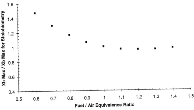
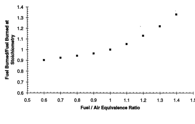
The other assumption with significant uncertainty is the value for air/fuel ratio of the inducted mixture. Fortunately, the results show a robustness similar to that of the total mass estimate described above. This can be seen in Figure 3.4. Lean Fuel/Air equivalence ratio estimates (less than 1) are seen to increase the maximum fraction burned. Unfortunately rich Fuel/Air ratio estimates have little effect on the burned fraction result. Figure 3.5 shows that the product of fuel in and fraction burned will stay nearly constant for estimates leaner than stoichiometric, but the fuel burned calculation will be significantly higher if the estimate is richer. The result is that if the actual vaporized fuel/air ratio is leaner than the estimate of stoichiometry, then the analysis is robust. Estimates 40% lean show a difference of less than 10% for the burned fuel result. Rich estimates of the same magnitude alter the fuel burned result by over 30%. Most

cycles during start-up seem to have lean vaporized Fuel/Air mixtures, even though the injected fuel/air ratio is rich, due to blowby and liquid fuel transport. If this is correct then the overall effect of the mixture composition estimate is minimal.

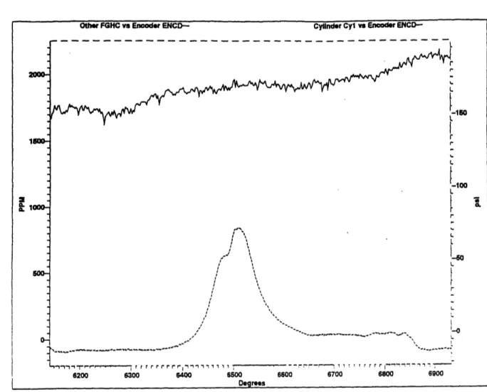
3.3 FEEDGAS HYDROCARBON MEASUREMENT

Each set of start-up data included output from a fast flame ionization type hydrocarbon detector. The probe was located in the collector pipe after the union of the exhaust manifolds and before the catalyst. The detector output was sampled 164 times per crankshaft revolution, and the signal was calibrated to parts per million (ppm) of

Propane (C3). The delay in the measurement system is believed to be very short, so the

ppm value for each cycle was taken to be the value of the sample at top center of the exhaust stroke. Figure 3.6 shows the typical variation of a feedgas hydrocarbon trace over the course of a cycle. To convert the ppm hydrocarbon value to a mass of fuel exhausted for that cycle, the molar fraction (ppm) value was converted to a mass fraction and multiplied by the mass of mixture for that cycle:

pprHC Mp~p

mmi x x - = mHc (3.2)

1,000,000 M=*

Where: mmix = the mass of mixture inducted that cycle

ppmhc = Hydrocarbon measurement value- parts per million Mpro = molecular weight of propane (44)

Mvexh = molecular weight of exhaust gasses (29) mhc = mass of hydrocarbons out

The uncertainty of this calculation is related to the variation and phasing of the ppm hydrocarbon signal. If the transport time for the exhaust gas does not correspond to the correct measurement being taken at top center then the estimate will be incorrect. The

magnitude of the error will depend on how rapidly the ppm signal is changing. Rapid changes that occur close to the fifth cycle may be 10% off, while slower changes will be less.

0.0 c.5 t.0 .5

PULSEW DTH (X) MSEC/PULSE

Figure 3.1 Fuel injector calibration curves for varying battery voltage. Higher voltage

produces faster solenoid operation, resulting in higher fuel flow for a given pulsewidth time. [Ford Motor Company]

r

I

1.0

0.8

0.6

0.4

0.2

I

I

CRANK ANGLE [deg]

0.03

0.02

0.01

0

-50

50

CRANK ANGLE [deg]

Figure 3.2 Sample profiles from the Bum Rate Analysis program. [Cheung]

I

r"

_-0

-

1.1 1.08 1.06 1.04 1.02 1 0.98 -0.96 -0.94 -0.92 -no U E . . . . . _. . 0.5 0.6 0.7 0.8 0.9 1 1.1 12 1.3 1.4 1.5

Mass Estimate/Original Mass Estimate

Figure 3.3 Effect of the Mass In estimate on the Fuel Mass Burned result. Large

changes in estimated charge mass result in less than 2% difference in the calculated burned mass. 1.6 1.4 1 *1 .2 -1 0.8 -0.6 . . a . . * * a . 0.6 0.7 0.8 C Fuel ).9 1 1.1

/ Air Equivalence Ratio

1.2 1.3 1.4 1.5

Figure 3.4 Effect of the Stoichiometry estimate on the Mass Fraction Burned result.

la₀ 3 1 LL _0 0 E o ._o n x x x

x

1.4 1.3 i 1.2

i3

m

1.1

Fuel / Air Equivalence Ratio

1.2 1.3 1.4 1.5

Figure 3.5 Effect of the Stoichiometry estimate on the Fuel Mass Burned result.

Differences in the output in the lean regime result in a much smaller change in output than mixtures on the rich side.

0.6 . .. . . .

,

I

F

Other FGHC vs Encoder ENCD-- Cylinder Cyl vs Encoder

ENCD-Figure 3.6 A sample Feedgas Hydrocarbon (HC) measurement showing

approximately 10% change in the engine-out HC reading over a complete engine cycle.

2000-15W 2 1000- 500-r L 1~ r . ~L L I~~~~~ I~~~~~- _r ' u1~~~~~~~~~~~~~~~~~~~~~~~~~~~~~~~~~~ _{\ ~~~~~~~~r}-10 i \} /} s 4~~~~~~~~~ 6200 6300 6400 6500 6600 6700 6800 6900 Degrees

CHAPTER 4 - FUEL ACCOUNTING

Now that the logic and uncertainties associated with the fuel and air modeling have been clarified, an explanation of the fuel accounting process will be given. This explanation will be done by going through an example using the 3.8 V6 data. The accounting is a cycle-by-cycle mass balance for the fuel, where the amount of fuel injected is compared with the amount burned or exhausted as unburned hydrocarbons. The difference is measured as "fuel unaccounted for".

4.1 FUEL INJECTED

A portion of a data trace showing the signal for the fuel injector along with the corresponding cylinder pressure (vs. time) is presented in Figure 4.1 (page 45). It can be seen that the injection process begins at the same point during each cycle. When the injection command drops below 2.5 volts the injector opens. To determine the fuel injected, the pulse width time signal is measured and converted to a corresponding fuel mass using the calibration curve described in Section 3.1. Figure 4.2 shows the mass of fuel injected for each cylinder during the V6 start-up. This is a sequential strategy, and not every cylinder receives the same amount of fuel during the same injection cycle. During the first engine cycle only half of the cylinders receive injections. In the second cycle there is a transition from very large injections to smaller pulses. The subsequent injections are approximately one seventh the amount of the original values.

4.2 FUEL BURNED

To calculate the amount of fuel burned during a cycle, several values must be estimated from the raw data. The burn rate analysis requires engine speed for the heat loss and residual sub-models. The calibration of the cylinder pressure trace and the

calculation of the charge mass requires the manifold pressure during intake for each cycle and cylinder. Figure 4.3 illustrates the points where the manifold and speed values were averaged: between bottom center of the intake stroke (BC) and intake valve closing (IVC) for the manifold pressure, and between intake valve closing (IVC) and bottom center (BC) of the expansion stroke for speed. This average manifold pressure was used in Equation 3.1 to calculate the total charge mass inducted for the cycle. The mass inducted, along with the average speed and manifold pressure, was then input to the bum rate program and the program was run for each cycle of each cylinder. The fuel burned determination was made by multiplying the mass of fuel inducted by the maximum fraction burned result obtained from the program. This is done for the first ten cycles of each cylinder, except for the V6 test where the first five cycles were analyzed due to problems with the data. For most cycles, the largest portion of the fuel was accounted for through burning.

4.3 HYDROCARBON OUTPUT

The calculation for the mass of engine-out hydrocarbons before the catalyst was based on the mass of charge in the cylinder and the feedgas hydrocarbon measurement at top center of the exhaust stroke for each cycle. Figure 4.4 presents the hydrocarbon trace for the 3.8L V6 with the corresponding mass of fuel exhausted as hydrocarbons for the first five cycles of one cylinder. The original signal contains a high frequency variation, but the trends are clear. There is a steady increase for the first five cycles, up to a maximum value exceeding 6000 ppm. The lower portion of the graph shows that this corresponds to approximately 0.0035 grams of fuel, or nearly one tenth the amount injected for a cycle at that point. It is interesting to note the two peaks that occur during

starting. This pattern was evident in almost all of the start-up data sets, including the warm start. One possible explanation for this trend is that the first peak is due to the

evaporation from these injections. Overall, the injected fuel that is accounted for by hydrocarbon output is a minor, but important fraction compared to the other components.

4.4 FUEL UNACCOUNTED FOR

For each cycle, the mass of fuel burned and the mass exhausted as hydrocarbons are subtracted from the mass injected. The balance is labeled "fuel unaccounted for", and represents fuel that remains in the intake manifold, is blown by the piston rings, absorbed into the oil, is in liquid form in the cylinder or is otherwise retained or lost by the

cylinder or port. It also may represent error in the fuel injected and fuel accounting computations.

The "fuel unaccounted for" can have a negative value due to fuel retention. For example, liquid fuel in the intake port that was injected during previous cycles may evaporate and make its way into the cylinder to supplement the current injection. In this case, the mass of fuel burned could be larger than the mass injected, resulting in a negative "unaccounted for" value.

Figure 4.5 shows a sample of the fuel accounting results for several cycles of one cylinder of the 3.8L V6. The first cycle shows that almost all the injected fuel is

"Unaccounted For" and there was no significant fuel burned. Cycle two displays a much smaller injection, with the mass burned close to 0.03 grams, while the hydrocarbon out value is less than one tenth of this. Some of the fuel injected during cycle one has been accounted for since the "unaccounted for" mass is negative. Cycle three shows little change in the burned mass and a slight increase in the HC Out mass from the previous cycle, but the "unaccounted for" value shifts to a positive value. Cycle four shows an

almost unchanged HC Out and "unaccounted for" mass. The burned mass decreases slightly along with the total mass.

By summing the fuel unaccounted for over each cycle, the cumulative mass of fuel unaccounted for is obtained. This representation gives insight to the fuel transport

behavior over several cycles. Figure 4.6 displays the result for the six cylinder sequential start. The traces begin with a large increasing slope and then level off. Two of the traces continue to increase substantially for a cycle beyond the others, indicating that they received an additional large injection of fuel. The portion of the curves with a flatter slope shows a slight decrease in unaccounted for fuel for most cylinders at first. After this point there is a minor increase. Overall, this graph shows that there is very little fuel recovered from the initial injections over the first several cycles. The mass of fuel "unaccounted for" after five cycles is between 0.15 and 0.35 grams for each cylinder, or the amount of fuel injected during approximately seven to fourteen cycles during idle.

Cylnde C· Ye 11mTM. te Niv ie IE

1250 1300 1350 1400 1450 1500 1550 1600 1650

msec

Figure 4.1 Sample cylinder pressure and fuel injection signals for one cylinder vs. time during a sequential start-up. Note that the injection starts at the same point in each cycle.

v

TIME--0.2 0.18 0.16 0.14 ' 0.12 " 0.1 · 0.08 0.06 0.04 0.02 0 K tR I A 1 2 3 Cycle

I

Figure 4.2 Mass of fuel injected for each cylinder in sequence (numbered) during the

3.8 L V6 start-up. v V x * " I---_ENEI-m :;iiiiii ii::

P

1

1p

Cylinder Cyl vs Encoder ENCD- Othr _MAP vs Encoder ENCD- Instantaneous RPM vs Encoder ENC

-I 460 400 300-P 250-a *, 150 .-1400 -1200 -1000 -80 R :-400 .-200 -O Degrees

Figure 4.3 A sample trace showing the location for the estimation of engine speed and

manifold pressure: Between bottom center (BC) and intake valve closing (IVC) for manifold pressure, and between IVC and BC of expansion stroke for speed.

1001 X 50 0-E ___ .

_yuae · y vs Enoe ENO thrfh v noerEJD !i ~L r

I0

iiuii

VtN.

Figure 4.4 A sample feedgas hydrocarbon trace plotted with one cylinder pressure trace vs. crankshaft degrees (above). Similar peaks occurred during most start-ups. The corresponding mass of fuel exhausted for one cylinder during the first five cycles.

3 2 2 11 10 $ 00- 50-Dl· 0-I i I ./. i' -5K OK ^ ^^^LI U.VU3OO 0.003 0.0025 cis 0 11_. 0.002 -0.0015 0.001 0.0005 - 0-1 0~T ---- 'NI7nn

Cynnoor " vsv Encoder ENC- Othr fghc vs Enodr

ENCD-i I II II I I I I . Y 1 i J~ I II

LI . 1 IM ~I 1 -I 1 1 [-1I l i191 I II 1 -I. II 1 - I. IlJ )'II IM "I ~ l J .i · i i Ll IJ IJ I I I l " l ~ J J l J i ~ I I 1 I l

I0.2 0.18 0.16 0.14 - 0.12-= 0.1-'I. o 0.08 -* 0.06 0.04 -0.02 0.0 -0.02

m

Figure 4.5 Fuel accounting results for the 3.8 L V6 start-up showing the mass of fuel

burned, output as hydrocarbons, and "Unaccounted For" during each cycle.

0.4 __ - 0.35 O 0.3 ° 0.25

0.2

o

Figure 4.6 Cumulative mass of fuel "Unaccounted For" for each cylinder of the 3.8 L

V6 start-up. The two higher traces are cylinders that receive two large pulses vs. only one for the other cylinders.

Cylinder 1 Cylinder 2 -* Cylinder 3 0- Cylinder 4 A-- Cylinder 5 -&-- .Cylinder 6 I I I I I 1

I

CHAPTER 5 - RESULTS AND DISCUSSION

The fuel accounting analysis method was applied to several sets of start-up data to provide a robust overview of the process and to observe differences in the starting

strategies. The engine start-up cases reviewed in this section include a simultaneous strategy, a sequential strategy, and a warm start using the sequential strategy. Each sample was chosen to be representative of data taken at similar conditions. A summary is given and conclusions are made about the effectiveness of the systems and strategies.

5.1 SIMULTANEOUS INJECTION

The majority of automobiles currently in production use the simultaneous injection strategy during starting. This provides quick starting with no additional engine position sensing necessary. However, since all injectors are fired with one command, there is no flexibility for different fuel needs between cylinders as the manifold pressure rapidly changes.

Figure 5.1 (page 61) shows the amount of fuel injected for each cylinder during the first ten cycles of a room temperature start of the 4.6 liter V8 engine using the simultaneous strategy. The first eight injections occur in the same point in time, but because of the timing of this injection in the firing order, the injection happens during either cycle one or two depending on the cylinder. One cylinder shows a slightly lower fuel mass for this injection, which is probably due to inaccuracies in the data acquisition and measurement process. The second eight injections are also simultaneous, and at about 0.13 grams, have a slightly lower mass. The third injection for each cylinder is distinctly different than the previous two. The mass drops to less than 0.02 grams,

almost one seventh the previous value, and the injections become sequential, although not every cylinder has injections occurring at the same relative point in the cycle yet.

cycle four to ten the fuel mass injected decreases by less than 0.01 grams. From Figure 5.1 the fuel strategy can be clearly seen: large initial injections followed by an immediate transition to smaller fuel pulses. Figure 5.2 shows how these pulses compare to the fuel required for the relative Fuel/Air ratio to equal one (a stoichiometric mixture) for one cylinder. Significant overfueling in the first two cycles is followed by slight

underfueling in the following seven shown.

Manifold pressure, engine speed, feedgas hydrocarbon level and the cylinder pressure of cylinder number one are presented in Figure 5.3 vs. crankshaft degrees. At least one misfire can be seen between cycles two and three in the initial acceleration of the speed trace, and the transition to idling speed near cycle four is rather abrupt, indicating poor combustion at this point. Poor combustion can also be seen as a rapid increase of the hydrocarbon output. The hydrocarbon output level peaks at a very high level, over 11,000 ppm C3, but no second peak is visible.

The normalized work output (IMEP/Pman) for each cylinder resulting from the injections is shown in Figure 5.4. Cranking cycles are seen as negative work output. Combustion is intermittent for the first cycle and a half, followed by the highest relative levels of work output. This high output is likely due to fuel that has accumulated from two injections. The variation of work output between cylinders generally decreases with the exception of the group of high output cycles and one cylinder in cycles eight and nine. Figure 5.5 displays the coefficient of variation (COV) for IMEP computed on an individual cycle basis. COVimep is the standard deviation of IMEP for all cylinders within a cycle, divided by the average IMEP value for that engine cycle, and expressed as a percentage. The first cycle is omitted since the majority are cranking cycles and COVimep has little meaning in this case. The second cycle shows a high value because not every cylinder has fired yet. The COVimep is close to 30 for cycles three to five, and drops lower thereafter. A COVimep above 10 is considered problematic for a

warmed-up engine, but for the early part of start-warmed-up a value below 20 by cycle five could be considered average.

Figure 5.6 displays the results of the fuel accounting analysis for one cylinder. The remaining cylinders show closely similar trends. The majority of the fuel injected during the initial large injections is "unaccounted for". Some of this "lost" fuel is accounted for in the following cycles, as evidenced by a negative "unaccounted for" mass. The mass of fuel burned increases slightly from cycle two to three, and then gradually decreases to about half of its peak value of 0.025 grams by cycle ten. Except for the first two injections, the burned mass accounts for the largest fraction of fuel injected, and by cycle eight the other portions are negligible. The hydrocarbon out mass increases to its largest values by the second and third injection (cycles three and four), and by cycle seven the amount is not visible in the figure.

The cumulative mass of fuel "unaccounted for" is shown for each cylinder in Figure 5.7. This is plotted by injection number (where one is the cycle before the first injection) instead of by engine cycle to avoid confusion due to the phasing of the first injection. Cylinders one and four are omitted because of problems encountered by the burn-rate program in analyzing one or more of the cycles for these cylinders. The trend of the data shows the large unaccounted for mass resulting from the first two large injections. The unaccounted mass for each cylinder peaks between 0.2 grams, and 0.24 grams, or approximately ten to twelve times the mass of one injection for cycle five (a "normal" sized injection). After the peak is reached, the unaccounted for mass begins to decrease, at first by close to 0.01 grams, then leveling out. The mass "regained", or "re-accounted for", by the end of ten cycles is around 0.02 grams, approximately 10% of the mass originally "lost", or about one "normal" injection.

This regained fuel is likely liquid fuel that has evaporated after being stored in the port or cylinder for one or more cycles. There are several possibilities for the fuel that