Coleman integration for hyperelliptic curves : algorithms and applications

Coleman Integration for Hyperelliptic Curves:

Algorithms and Applications

by

Jennifer Sayaka Balakrishnan

A.B., Harvard University (2006)

A.M., Harvard University (2006)

ARCHNvES

MASSACHUSETS INSTITUE

OF TECHNOLOGY

=SEPP

0

2 2011

L-LI BRA-R iEF-s

Submitted to the Department of Mathematics

in partial fulfillment of the requirements for the degree of

Doctor of Philosophy

at the

MASSACHUSETTS INSTITUTE OF TECHNOLOGY

June 2011

@

Jennifer Sayaka Balakrishnan, MMXI. All rights reserved.

The author hereby grants to MIT permission to reproduce and

distribute publicly paper and electronic copies of this thesis document

in whole or in part.

A uthor ... ... . . ...

Department of Mathematics

April 26, 2011

Certified by ...

.2. . . ... ...

Kiran S. Kedlaya

Associate Professor

Thesis Supervisor

Accepted by ... .. !. O...

Bjorn Poonen

Chairman, Department Committee on Graduate Theses

Coleman Integration for Hyperelliptic Curves:

Algorithms and Applications

by

Jennifer Shyamala Sayaka Balakrishnan

Subnitted to the Department of Mathematics on April 26, 2011, in partial fulfillment of the

requirements for the degree of Doctor of Philosophy

Abstract

The Colemani integral is a p-adice line integral that can be used to encapsulate several quantities relevant, to a study of the arithmetic of varieties. In this thesis, I describe algorithms for computing Coleman integrals on hyperelliptic curves and discuss some immediate applications. I give algorithms to compute single and iterated integrals on odd models of hyperelliptic curves, as well as the necessary modifications to iplemieit these algorithms for even models. Furthermore, I show how these algorithinis can be used in various situations. The first application is the method of Chabatv to find rational points on curves of genus greater than 1. The second is Mlihyong Kim's recent nonabelian analogue of the Chabauty method for elliptic curves. The last two applications concern p-adic heights on Jacobians of hyperelliptic curves. necessary to formulate a p-adic analogue of the Birch and Swinnerton-Dyer conjecture. I conclude

by stating the analogue of the Mazur-Tate-Teitelbaum conjecture iii our setting and

presenting supporting data.

Thesis Supervisor: Kiran S. Kedlaya Title: Associate Professor

Acknowledgments

It is a pleasure to thank my advisor, Kiran Kedlaya, for his support of the efforts that went into this thesis. He has been incredibly generous with his time and ideas, patiently answering my numerous questions, suggesting many interesting problems, and encouraging several collaborations. One such collaboration led to the results in Chapter 3, which form the backbone of this thesis.

I would also like to thank a few others who have had a direct impact on this

the-sis. During rny first year in college, I happened to take a seminar with William Stein, who introduced me to computational approaches in number theory. Over the years, we have worked on a few things together - most recently, a portion of the material that forms Chapter 9 of this thesis. Special thanks must also go out to two of my coauthors, Minhyong Kirn and Amnon Besser, who kindly explained their work to me; collaborations with them led to Chapters 7 and 8, respectively, of this thesis. Thanks are also due to Barry Mazur, Bjorn Poonen, Alice Silverberg, Michael Stoll, Drew Sutherland, and Liang Xiao, for several productive discussions, and Robert Bradshaw and David Roe for laying much of the p-adic groundwork in Sage.

I must also thank Steffen iller for visiting MIT last summer arid carefully computing (and recomputing) many things in Magma, despite the many ill-posed queries I came up with during the process. It would have been impossible to assen-ble the data in Chapter 9 without his efforts. Repeating names, I would also like to thank Bjorn Poonen, Abhinav Kumar, and Kiran Kedlava for agreeing to serve on rny thesis cornnittee, William Stein for access to his cluster of computers (chief among then {mod, boxen, sage}.math.washington.edu, funded by NSF grant

DMS-0821725), and Kiran Kedlaya for access to dwork.mit .edu.

Finally, to my dear friends and family, thank you for your love, laughter, and sup-port throughout the years. Kartik arid Liz, I have thoroughly enjoyed our adventures in baking arid ballet. And above all, Bala, Shizuko, Stephanie, and Vivek, thank you for always cheering me on, regardless of the time or time zone.

This research was supported by the National Science Foundation Graduate Re-search Fellowship and the National Defense Science arid Engineering Graduate Fel-lowship.

For those in Yamada,

Contents

1 Introduction 15

1.0.1 Why hyperelliptic curves?...

. . . ..

1)

1.0.2 Beyond lyperelliptic curves'? . . . . 16

1.0.3 Outline ... . . . . . . . . . 16

2 Hyperelliptic curves and p-adic cohomology 19 2.1 Hyperelliptic curves... . . . . . . . . 19

2.2 p-adic cohonology . . . . 21

2.2.1 Frobenius... . . . . 23

2.2.2 Kedlaya's algorithm... . . . . . . . . 23

3 Coleman integration: the basic integrals 27 3.1 Coleman's theory of p-adic integration . . . . 27

3.2 Explicit integrals for hyperelliptic curves . . . . 29

3.2.1 A basis for de Rham cohonology . ... 30

3.2.2 T iny integrals . . . . 30

3.2.3 Non-W eierstrass disks . . . . 31

3.2.4 Weierstrass endpoints of integration ... 34

3.3 Implementation notes and precision . . . . 36

3.3.1 Precision estim ates . . . . 36

3.3.2 Complexity analysis . . . . 37

3.3.3 Numerical examples . . . . 38

4 Coleman integration: even degree models 41 4.1 Introduction . . . . 41

4.2 A bit more p-adic cohomology . . . . 41

4.3 Coleman integration on even models . . . . 42

4.3.1 Local coordinates . . . . 42

4.3.2 Integrals . . . . 42

4.3.3 Using the linear system . . . .. 44

5 Coleman integration: iterated integrals 47 5.1 Introduction . . . . . .. .47

5.2 Iterated path integrals . . . . 48

5. 3.1 Examples . . . . . . . . .

5.4 Iterated integrals: linear system... . . . ...

5.5 Explicit double integrals . . . ...

5.5.1 Tiny double integrals . . . .

5.5.2 The linear system for double integrals between Teichnffller points

5.5.3 Linking double integrals . . . . 5.5.4 Without Teichinliler points . . . .

5.5.5 W eierstrass points . . . .

5.6 Future w ork . . . .

5.6.1 Tangential basepoint at infinity . . . .

5.6.2 The fundamental linear system . . . .

5.6.3 The region of convergence in a Weierstrass disk . . . .

6 Explicit computations with the Chabauty method 6.1 Introduction... . . . . . . . . . .. 6.2 Explicit integrals to a parameter . ...

6.3 Example: odd model.... . . . ..

6.4 Future work . . . .

7 Kim's nonabelian Chabauty method 7.1 Introduction: the method...

7.1.1 Elliptic curves. . ....

7.2 A few moire explicit double integrals .

7.2.1 Integrals to a parameter z

7.2.2 Double integrals to a parameter

7.3 Carrying out the nonabelian Chabauty met

7.3.1 An example with 65A . . . . 7.3.2 An example with 37A

7.4 Connection to p-adic heights . . . .

7.5 Future work . . . .

7.5.1 Tangential basepoint . . . .. 7.5.2 Tamagawa number hypothesis

hod 73

73

74

-6 7 7 78

80

81 81 81

83

83 84

89

90 90

90

93 99 99 100 100 8 p-adic heights on Jacobians of hyperelliptic curves

Q 1 I t d t 8.2 The p-8.3 Hypere 8.4 Colem 8.4.1 8.4.2 8.5 The lo 8.5.1 8.5.2 8.5.3 8.5.4

adic height pairing . . . . Iliptic curves. . . . . . . . ..

an integrals . . . . Generalities on Coleman integrals and symbols Integration of forms with poles outside Weierstrass cal height pairing at primes above p . . . .

Computing cup products . . . . The m ap T . . . . Decomposing a divisor D into D' and D"l . . . A form with the required residue divisor . . . . .

8.5.5 8.5.6 8.5.7 8.5.8 8.5.9 Finding wJD for a Finding WD for a Integration when Computation wh Computation wh Weierstrass divisor D... . . . .

.

non-Weierstrass divisor D...

D2 reduces to W'eierstrass points

en

Di

is Weierstrass and D2 is not

en both divisors are non-Weierstrass

.

. .

.. .

.

.

. . . .

. .

8.6 Implementation notes .

8.6.1 Auxiliary choices.. ...

8.6.2 Precision... . . . . . . . .. 8.7 Exam ples . . . .

8.7.1 Local heights: genus 2, general divisors...

8.7.2 Local heights: oenus 2 anti-symnetric divisors

8.7.3 Global heights: genus I...

8.7.4 Global heights: genus 2 ...

8.8 Future work... . . . . . . . .. 8.8.1 Global height pairings. ...

8.8.2 Optimizations.. . . . . . . .. 8.8.3 Comparison with the work of Mazur-Stein-Tate

9 A p-adic Birch and Swinnerton-Dyer conjecture

9.1

Introduction . . . .

...

9.2

p-adic height pairings and regulators...

. . ..

9.3

p-adic L-series . . . ...

9.3.1

Inert case . . . . .

...

9.3.2

Split case . . . ...

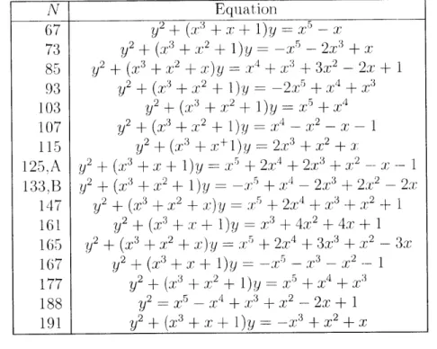
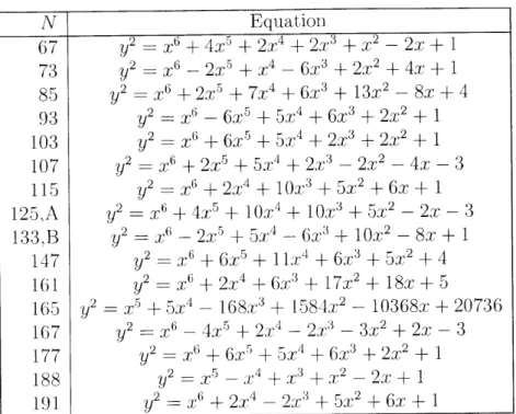
9.4 Data for rank 2 Jacobians of genus 2 curves...

. .

.

9.4.1

Auxiliary data...

. . . .

. . ..

9.4.2

Evidence for Conjecture 9.1.4. . . .

. . . ..

9.4.3

Future work . . . .

A Auxiliary p-adic BSD data

A.1 N=67.

A.2

A.3

A.4

A.5

A.6

A.7

A.8

A.9

A.10

A.11

A.12

A.13

A.14

N = 73.

N = 85 .

N = 93. N = 103 N = 107 N = 115 N = 125,

N

= 133,

N = 147

N = 161 N = 165

N = 177

N = 188

A.15 N = 191 101 101 101 101 101 101 102 102 106 106 107 109 110 110 110 111 111

113

115

1 16 116 118

1 19

119 121 141

143

143 146 147 148 150 152 154 156 157 159 160 162 165 167 169

. . . .. .

. . . .I

. . . .. . . . .

. . . .. . . . .

. . . .

. . . .

. . . .I

. . . .

. . . .

. . . .. .

. . . .

. . . .

List of Figures

3.1.1 Residue disks on an elliptic curve... . . . . ... 28

3.1.2 A wide open subspace . . . . 28

3.2.1 A tiny integral between P and

Q.

. . . .

31

List of Tables

9.4.1 Levels and integral models (Table 1, [FpS+01])... 119

9.4.2 Levels and

y

2 =

f(x)

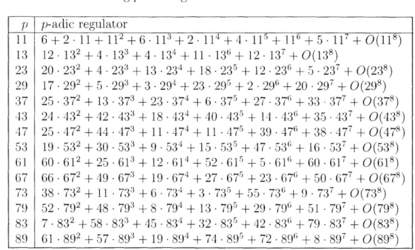
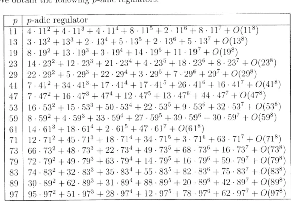
models . . . . 120

9.4.3 BSD data for rank 2 Jacobians of genus 2 curves (Table 2, [FpS+01]) 120 9.4.4 Global generators and itersection data (computed by Steffen Mnller) 121 9.4.5 p-adic regulators, N = 67 . . . . 123

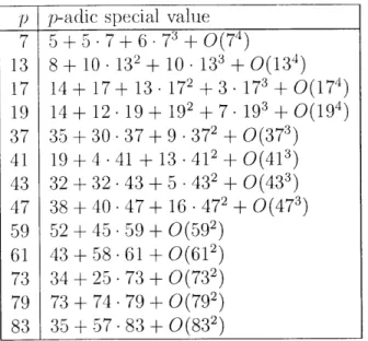
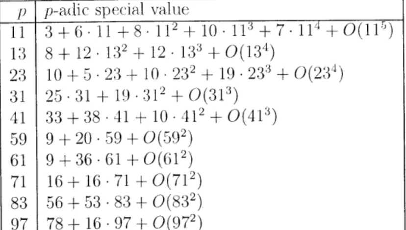
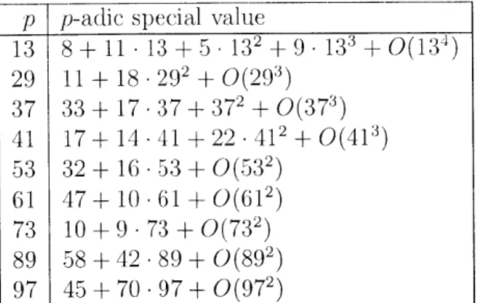
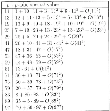
9.4.6 p-adic special values, N = 67 . . . . 123

9.4.7 p-adic regulators, N = 73 . . . . 124

9.4.8 p-adic special values, N = 73 . . . . 124

9.4.9 p-adic regulators, N = 85 . . . . 125

9.4.10 p-adic special values, N = 85 . . . . 125

9.4.11 p-adic regulators, N = 93 . . . . 126

9.4.12 p-adic special values, N = 93 . . . .. 126

9.4.13 p-adic regulators, N = 103 . . . . 127

9.4.14 p-adic special values, N = 103 . . . . 128

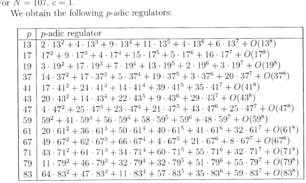
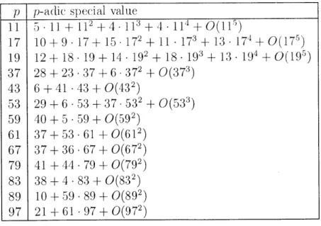
9.4.15 p-adic regulators, N = 107... . . . .. 129

9.4.16 p-adic special values, N = 107 . . . . 129

9.4.17 p-adic regulators, N = 115 . . . . 130

9.4.18 p-adic special values, N = 115 . . . . 130

9.4.19 p-adic regulators, N = 125, A . . . . 131

9.4.20 p-adic special values, N = 125, A . . . . 131

9.4.21 p-adic regulators, N = 133, B . . . . 132

9.4.22 p-adic special values, N = 133, B . . . . 132

9.4.23 p-adic regulators, N = 147 . . . . 133

9.4.24 p-adic special values, N= 147 . . . . 133

9.4.25 p-adic regulators, N = 161 . . . . 134

9.4.26 p-adic special values, N = 161 . . . . 134

9.4.27 p-adic regulators, N = 165 . . . . 135

9.4.28 p-adic special values, N= 165 . . . . 136

9.4.29 p-adic regulators, N = 177 . . . . 137

9.4.30 p-adic special values, N= 177 . . . . 137

9.4.31 p-adic regulators, N = 188 . . . . 138

9.4.32 p-adic special values, N= 188 . . . . 139

9.4.33 p-adic regulators, N = 191 . . . . 140

9.4.34 p-adic special values, N= 191 . . . . 140

A.2.1 a factors for N 73 . . . . 146

A.2.2 e factors for N 73 . . . . 146

A.3.1 a factors for N 85 . .... ... .. ... 147

A.3.2

c

factors for N

85 . . . .

147

A.4.1 a factors for N 93 . . . . 148

A.4.2 c factors for N 93 ... .... .. ... 149

A.5.1 a factors for N 103 . . . . 150

A.5.2 c factors for N 103 . . . . 151

A.6.1 a factors for N 107 . . . . 152

A.6.2 e factors for N 107 . . . . 153

A.7.1 a factors for N 115 . . . . 154

A.7.2 e factors for N = . . . . 155

A.8.1 a factors for N 125, A . . . . 156

A.8.2 c factors for N = 125, A . . . . 156

A.9.1 a factors for N 133, B . . . . 157

A.9.2 C factors for N - 133, B . . . . 158

A.10.1a factors for N 147 . . . . 159

A.10.2c factors for N = 147 . . . . . 159

A.11.1a factors for

N

161... . . . .. 160

A.11.2c factors for N 161 . . . . 161

A.12.1a factors for N 165 . . . . .163

A.12.2e factors for N = 165 . . . . 164

A.13.1a factors for N 177 . . . .. . 65

A.13.2e factors for N 177... . . . . . . . ... 166

A.14.1a factors for N 188 . . . .. 167

A.14.2c factors for N 188 . . . . 168

A.15.1a factors for N 191 . . . . 169

A.15.2c factors for N 191 . . . . 169

Chapter 1

Introduction

The Coleman integral is an analytic tool that serves as the p-adic analogue of the usual (real-valued) line integral. These p-adic integrals help us understand the arithmetic and geometry of curves and abelian varieties. For example, certain integrals allow us to find rational points or torsion points; certain others give us p-adic height pairings.

Constructing this p-adic analogue is not at all obvious, as the totally disconnected topology of p-adic spaces makes it difficult to introduce a neaningful forim of olobal antidifferentiation. Nevertheless, in a series of papers in the 1980s, Robert Coleman circumvented this problem using Dwork's principle of Frobcnius equiva riance. Using this idea, Coleman introduced a p-adic integration theory first on the projective line [Col82], then (partly jointly with de Shalit) on curves and abelian varieties [Col85],

[CdS88].

Since then, alternative treatnents have been given by Besser [Bes02a] using nethods of p-adic cohomology, and by Berkovich

[Ber07]

using the nonarchiniedean Gel'fand transform.

It was not immediately obvious that Coleman's p-adic integration theory was suitable for wide-scale computation. The first implementation (due to Besser and de Jeu [BdJ08]) was for curves of genus 0. In 2001, Kedlaya [Ked0l] gave an algorithm computing the action of Frobenius on appropriate cohomology groups of hyperelliptic curves and in 2007 demonstrated [BCD+08] that this algorithm could realize the Frobenius equivariance necessary for computing global Coleman integrals on such curves.

Motivating these algorithms is the fact that Coleman integration plays an impor-tant role in a study of the arithmetic of curves and abelian varieties. For example, appropriate integrals allow us to find torsion points and certain others describe in-tegral points. Yet others give us a means to compute p-adic heights and regulators. Explicitly computing these quantities serves as motivation for several of our algo-rithms.

1.0.1

Why hyperelliptic curves?

The key input for all of our Coleman integration algorithms is the matrix of the action of Frobenius on an appropriate cohomology group of the variety. In particular, given a curve C, what is necessary is an algorithm that can compute the action of

a p-power lift of Frobenius on a differential and then "reduce"' it within the first de Rhan cohoiology group of the curve, HR,(C): that is, express it in terms of an exact differential plus a linear combination of basis (or pseudo-basis) differentials of

H(, R(C).

Since Kedlaya's algorithm [Ked01], which does precisely this, was originally pur-posed for hyperelliptic curves (and p > 2), the class of hyperelliptic curves was a natural starting point for our integration algorithms. Moreover, several applications of Coleman integration concern Jacobians of curves of genus greater than 1. Jacobians of hyperelliptic curves provide many interesting examples.

1.0.2

Beyond hyperelliptic curves?

Nevertheless, since Kedlaya's work, several generalizations have been formulated. Denef and Vercauteren [DVOG] extended Kedlaya's algorithm to hyperelliptic curves in characteristic 2. Subsequent work by Gaudry and Girel [GG01] treated the case of superelliptic curves. Castryck, Denef, and Vercauteren [CDV06] generalized Ked-laya's algorithm to nondegenerate curves. Any of these algorithms could be used to give Coleman integration algorithms on the relevant classes of curves. Moreover. the work of Abbott-Kedlaya-Roe [AKR09] (riot to mention. David Harvey's recent optimriized version [Har10b]), which does the analogous task for snooth hypersurfaces in projective space. could be used to ext end Coleman integration beyond curves. It should also be possible to compute Coleman integrals using Frobenius structures on Picard-Fuchs (Gauss-Manin) connections, extending Lauder's deforma[ion method for conputing Froberius matrices [Lau04].

1.0.3

Outline

This thesis presents several algorithms for p-adic integration on hyperelliptic curves. We begin with an introduction to hyperelliptic curves and Kedlaya's algorithm for computing the action of Frobenius on their cohomology. In Chapter 3, we rise this to give algorithms to compute single Coleman integrals on odd models of hyperelliptic curves of good reduction over C, for p > 2, as first appeared in joint work of the author with Bradshaw and Kedlaya [BBK10]. Chapter 4 builds on the work of Harrison

[Harl0a] to extend our techniques to even models of hyperelliptic curves. Chapter 5

presents algorithms to handle iterated Coleman integrals, with an emphasis on the

particular case of double Coleman integrals.

The subsequent chapters of this thesis deal with applying these methods to study

problems of interest in arithmetic geometry. In

Chapter 6, we give an exposition of

the method due to Chabauty and Coleman to find rational points on higher genus

curves and demonstrate our algorithms in the case of hyperelliptic curves. Chapter

7

highlights Kim's recent work on a nonabelian analogue of this method as well as a

few more algorithms and a behind-the-scenes look at numerical examples that first

appeared in joint work of the author with Kedlaya and Kim in the Appendix and

Erratum to [Kiml0a]. In Chapter

8,

we discuss the techniques of Coleman and Gross

in joint work with Besser

[BB]

which adapt previous Coleman integration techniques to allow for differentials having residue divisors with non-Weierstrass support. This work gives the first algorithm to compute the Coleman-Gross local height pairinlg for Jacobians of hyperelliptic curves. Finally, we conclude in Chapter 9 with joint work of the author, Miller and Stein on explicit computations of p-adic regulators and p-adic L-series associated to Jacobians of hyperelliptic curves. We present some evidence toward a higher-dimensional analogue of the p-adic Birch and Swinnerton-Dyer conjecture.

Throughout, our algorithms have been implemented in the Sage computer algebra system [S+11]. It is our hope that this thesis will serve as an introduction to the vast landscape of explicit methods involving p-adic integration.

Chapter 2

Hyperelliptic curves and p-adic

cohomology

Ve begin by recalling some facts about hyperelliptic curves

[CF05].

We continue with an introduction to some tools from p-adic cohonology, following the exposition in [CF05), as well as previous joint work of the author with Bradshaw and Kedlaya [BBK1O]. These foundations will allow us to formulate the Coleman integration algorithms in subsequent chapters of this thesis.

2.1

Hyperelliptic curves

Let K be a field of characteristic not equal to 2.

Definition 2.1.1. A hyperelliptic curve C/K is a smooth projective curve of genus

g > 1 such that, an affine model of C can be written as

y2

=

f

(X),

f (x)

E K[x],

with deg(f) < 2g + 2.

Let t denote the hyperelliptic involution t : (x, y) k (x, -y).

Definition 2.1.2. The Weierstrass points P1..., P2, 2 are the K-rational fixed points of t.

A point that is not a Weierstrass point is a

non-

Weierstrass

point.

If deg

f

(x)

2g

+

2, then there are two distinct K-rational non-Weierstrass points P+, P"- lying over oc. If deg f(x) = 2g + 1, then there is a single Weierstrass point P, at oC.

If

f(x)

has a K-rational root, we may apply yet another change of coordinates to obtain a model of the form

y =f(x), deg

f

(x) = 2g

+

1.

We refer to this as an odd model for C. We distinguish between this case and that of the even model: when the curve is of the form y2 =

f(x)

with deg

f (x) = 2g + 2.

Unless otherwise mentioned, for sirmplicity, we present our algorithms for odd m1od-els of hyperelliptic curves and shall henceforth assume that deg f(x) = 2g + 1. In

Chapter 4, we suspend this restriction and specifically address the situation of even models.

Let K(C) denote the field of rational functions of C. Recall that a local parameter or a local coordinate at a K-rational point P is a function t E K(C) such that ordp(t) = 1. Having explicit local coordinates at points on C is crucial to our integration algorithms. Here we record our local coordinate algorithms:

Algorithm 2.1.3 (Local coordinate at a non-Weierstrass point).

Input: A non-Weierstrass point P = (a, b) on C (with b

$

0) and precision n.

Output: A parametrization (x(t), y(t)) at P in terms of a local coordinate.

1. Let x(t) = t

+

a, where t is a local coordinate.

2. Solve for y(t) -

f(x(t))

by Newton's method: take yo = b, then set

yi=

(yi1

, z>1

2

y41M

with yj (t) -+ y(t). The nuirner of iterates i to be taken depends oii the iecessary power series precision; for precision O(t"), one can take 1 to be [log2 "

Example 2.1.4. Let C be the hyperelliptic curve y2 = x5 - 23x 3 + 18r2 _{+ 40x and}

consider the point P = (1, 6) on C. Then the local coordinates (x(t) , y(t)) at P are

x(t) = 1 + t,

7

13

254

y(t) = 6+t

- -t2 _ _t

-2 t4 +

0(t 5 ).

2

2

48

Algorithm 2.1.5 (Local coordinate at a finite Weierstrass point).

Input: A finite Weierstrass point P = (a, 0) on C and precision n.

Output: A parametrization (x(t), y(t)) at P in terms of a local coordinate.

1. Let y(t) = t where I is a local coordinate.

2. Iteratively solve for x(t). One way is as follows: since

f(a)

= 0, note that g(x) :=

f(x)/(x -

a)

is a polynomial in x. Take

1 xo= a

+

t2

g(a)

let h(x, t)

f(x)

- t2, and compute h'(x, t) =h-c,) Newton's method yields_ax x +I) -= xiMt) -_(xi (t), t)

with xi (t) -+ x(t). The number of iterates i to be taken depends on the necessary power series precision; for precision

O(t"'),

one can take

i

to be [log2 nl

Example

2.1.6. Let

C

be the hyperelliptic curve

y2

= 5-23x3 + 18X2

+

40x and let P = (4, 0) on C. Then the local coordinates (x(t),

q(t))

at P are

1

1 _{191 4}

₇₅₇₉

+0(t 7_), 360 23328000 188956800000

y(t) = t.

Finally for the case of infinity, since y2

=

f

(x), where

deg

f

(x) = 2g +

1, we have

that x has a pole of order 2 at oo, while y has a pole of order 2g + 1 at o. Let t be the local parameter at cc. To find the parametrization, we do as follows:

Algorithm 2.1.7 (Local coordinate at infinity).

Input: The point

P,

above

x = o

on

C

and precision n.

Output: A local coordinate (x(t), y(t)) at P, such that t has a zero at c.

1. Take

X0 = t-2

let h,2(x, t) = +f

f/x)

and compute

['(x,

t) = h3x. Newton's metliod yields

h(x

1

(t), t)

with x(t) -+

x(t).

The number of iterates i to be takein depends on the necessary power series precision; for n digits of precision in t, i can be taken to be [log2 o.

2. Take y(t) = (x(t)).

Example

2.1.8. Let

C

be the

iyperelliptic

curve y2 _{=X - 23X3}

+ 18x2

₊

_{40x. At oc,} we have x(t) = t-2 ₊

_23t

2 _{- 18t}4 - 569t' + 0(t 7),

y(t) = t-

+

46t-

-

36t

-

609t3 + 16,56t" + 0(t6)

2.2

p-adic cohomology

To discuss the differentials we will be integrating, we briefly introduce the necessary p-adic cohomology and sone core definitions from [KedO 1]. Let p > 2g - 1 be a prime and K an unramified extension of

Q,.

Let C/K be a curve with good reduction. We will assume in addition that, we have been given a model of C of the form y2 ₌

_f(X)

with

f(x)

having coefficients in the valuation ring 0 K of K. We will assume that the leading coefficient, of

f

is a unit, that (leg f(x) 29 + 1, and that

f

has no repeated roots modulo p. Let C' be the affine curve obtained by deleting the Weierstrass points from C. Let A = K[x, y, z]/(y2 _-

_f(x),

_yz

_{1) be the coordinate ring of C'.}

Definition 2.2.1. The Monsky-Washnitzer (MW) weak completion of A is the ring

At consisting of infinite sums of the form

Bi(x)

3

Bi

(x)

C

K[x], deg Bi < 2

,

further subject to the condition that vp(Bi(x)) grows faster than a linear function of

i as i -s ±oo. We make a ring out of these by using the relation y2 _f(X).

Associated to each element h

E

At is a differential dh such that the Leibniz rule holds: d(hg) = h dg+q dh and such that da = 0 for each a

C

K. Let (2 be the module of these differentials: then the operator d defines a K-derivation from At to 2. Since

y2

-

f(X) =

0,

we

conclude

that

dy

f'(x)

and thus .2= At d.

2y 2y

Let,

H7R (C) = ker(d) ={h CAt

Idh

= 0}, HjiR(C)

= coker(d)

=

(At

(d t)

Thus elements of HjR(C) are differentials modulo exact, differentials dh for soni

h

E

At. The next leinia [IKed0l, @3] gives a basis for Hja(C').

Lemma 2.2.2. The

first

de Rham

cohomoloqy

H

j(C')

splits into eigenspaes under

the hyperelliptic involution

/:

* a positive eigenspace H

jR(C')+

with basis {x'

k}

for i

= 0,... , 2g.

e

a

negative eigenspace Hj(C')~ with basis

{x'

}

for

i = 0, . .. ,29 - 1.

For reasons which will become clear in the next chapter, we focus our attention on 1-forms that are odd, i.e., which are negated by the hyperelliptic involution. Let

dx

wki =

x~i

(i =0,)

2g - 1).

(2.2.1)

2y

By the lemma above, any odd differential w E 2 can be written uniquely as

o= df

+

cowo + - + C2g-1W2g-1

(2.2.2)

with

f

E At and c, E K, since the w-j form a basis of the odd part of the de Rham cohomology of At. The process of putting w in the form (2.2.2), using the relations

y2

d(x'ya) =

(21i-

yj+1

+

jif(x)yj-,)

d ,

can be imade algorithmic; this is Kedlaya's algorithm, which we describe below. (Briefly, one uses the first relation to reduce high powers of x, and the second to reduce large positive and negative powers of y.)

2.2.1

Frobenius

Since K is an unramified extension of

Qp,

it carries a unique automorphism

#K

lifting the Frobenius automorphism x x xP on its residue field. Extend

#K

to a Frobenius lift

#

on At by setting

OW XI),

(Y)

+

O(f)(x) -

f(X)P)

1/2

Y (1/2) -

f(x)P)1

i=0i

We will also need (y)', which can be cornputed as

1/2 (fx - f(x)P)i

i=0i

RCrmark 2.2.3. Note that one needs y- as an element of At. which explains why we conpute with C' instead of C.

Note also that for ease of exposition, we describe all of our algorithms as if it were possible to compute exactly in At. This is not possible for two reasons: the elements of At correspond to infinite series, and the coefficients of these series are polynomials with p-adic coefficients. In practice, each cornputation will be made with suitable p-adic approximations of the truly desired quantities, so one must keep track of how much p-adic precision is needed in these estimates in order for the answers to bear a certain level of p-adic accuracy. We postpone this discussion to

53.3.1.

2.2.2

Kedlaya's algorithm

To compute in H),1(C), we need to express an arbitrary differential form as the sum of a K-linear combination of the basis in Lemma 2.2.2 and an exact differential. We refer to this process as reduction in cohomology and carry it out as follows.

First note that any differential form can be written as O 2g

ajk

dx,

a&

aL. c

K.

k=-oc i=O

Indeed, using the equation of the curve, we can replace h(x)f(x) with h(x)y 2 as many times as needed. Next, a differential )

dx

with P(x) E K[x) and s E N

can be reduced as follows. Since J(x) has no repeated roots, we can always write

P(x)

=

U(x)f(x)

+

V(x)f'(x). Since d

(> )

is exact, we obtain

P(x)

_PWdx=

dx

(V'x

_U

_x)+ + xi

)

dx-2

_d

y S s -2 )y s-2'

where = means equality rnodulo exact differentials. This congruence can be used to reduce a differential form involving negative powers of y to the case = 1 and s = 2. Moreover, a differential )

dx

with deg P = n > 2g can be reduced by repeatedly

subtracting appropriate multiples of the exact differential d(xi -29,) for i

n,

... , 2g.

Finally, note that the differential P dx is congruent to ( x mod f (x) dx niodulo exact

differentials. A differential of the form P(x)y" dx with P(x) E K [x] and s e N is exact if s is even and equal to dx if s is odd and thus can be reduced using the above reduction formula.

Since the q-power Frobenius

#4

is

#d,

it suffices to cornpute the matrix Ml through which the p-power Frobenius acts on the anti-invariant part HdR(C) of HJ(() te

iatrix of the q-power Frobenius can then be obtained as A =fM(MJ) - . -(M\).

The action of 6 on the basis of H'R(C> (an be computed as

#

dx

1X

=

dx,

2( 26(y)

for i 0. 2g -- 1. Given a sufficiently precise approximation to . we caII use

reduction in cohoiology to express

#(wi)

on the basis of Hj'(C)~ and coimpute the

matrix Ml. This is Kedlaya's algorithm:

Algorithm 2.2.4 (Kedlaya's algorithm). Input: The basis differentials (og)2,.

Output: Functions

fi

e At and a 2g x 2g matrix M over K such that 29-1

) df

+

E

>3Mip

j=0

for all i.

1. Compute

#(x), #(y)

as infinite series in At.

2. Use a Newton iteration to compute 0. Then for i = 0,...,2g - 1, proceed as in @'2.2.2 to write

-*(wi)

=

px""' 9

= df' +

gM- 1 (2.2.3)

0(y) 2y .

For sone applications, it may be convenient to use a

different

basis of de

Rharm

cohomology.

For instance, the basis d(i 0,... ,2g - 1) is crystalline (see

[Harl0a], as well as the erratum to [KedOl), so Frobenius will act via a iatrix with

p-adically integral entries.

Chapter 3

Coleman integration: the basic

integrals

Most of the material in this chapter originally appeared in joint work of the author with Bradshaw and Kedlaya [BBK1O].

3.1

Coleman's theory of p-adic integration

In this section, we recall Coleman's p-adic integration theory in the case of curves with good reduction. This theory involves some concepts from rigid analytic geon-etry which it would be hopeless to introduce in such limited space: some standard

references are [BGR84) and [FvdP04]. (See also [Col85,

1).)

Let C, be a completed algebraic closure of

Qp,

and let 0 be the valuation subring

of CP. Choose once and for all a branch of the p-adic logarithm, i.e., a homomorphism

Log : C' -* C, whose restriction to the disk

{x

E C, : Ix - 11 < 1} is given by the logarithm series log(x) I- -(1 x)'/i. (The choice of branch will have no

effect on the integrals of differentials of the second kind, i.e., everywhere meromorphic differentials with all residues zero.)

We first introduce integrals on disks and annuli within IP.

Definition 3.1.1. Let

I

be an open subinterval of [0,+o0). Let A(I) denote the

annulus (or disk) {t E

:

It|

E I}. For

eZcit'dt E

I

and P, Q E A(I),

define

cit' dt c_1Log(Q/P)

+

>3

N

-

.

iEZ i:7 -I

This is easily shown not to depend on the choice of the coordinate t.

Remark 3.1.2. Note that because of the division by i+1 in the formula for the integral, we are unable to integrate on closed disks or annuli (as this affects convergence on the "boundary").

Definition 3.1.3. By a curve over 0, we will mean a smooth proper connected

scheme X over 0 of relative dimension 1. Equip the function field K(X) with the p-adic absolute value, so that the elements of K(X) of norm at most 1 constitute the local ring in X of the generic point of the special fibre X of X.

Let X " denote the generic fibre of X as a rigid analytic space. There is a natural reduction map from X " to X(Fp); the inverse image of any closed point of X is a subspace of Xa" isomorphic to an open unit disk. We call such a disk a residue disk

of X.

Figure 3.1.1: Residue disks on an elliptic curve

re7 P

r/

'I~

~

e d.

'& 'F'

Definition 3.1.4. Let X

will mean a rigid analytic finite collection of disjoint

be a curve over 0. By subspace of Xa" that is

closed disks of radius AN

a wide open subspace of X", we

the complement of the union of a

< 1.

Figure 3.1.2: A wide open subspace

Coleman made the surprising discovery that there is a well-behaved integration theory on wide open subspaces of curves over 0, exhibiting no phenomena of path

Xza

5 _M

dependence. (One needs to consider wide open subspaces even to integrate differ-entials which are holomorphic or reromorphic on the entire curve.) In the case of hyperelliptic curves, Coleman's construction of these integrals using Frobenius lifts will be reflected in our technique for computing the integrals. For the general case, see [Col85, @2], [Bes02a, @4], or [Ber07, Theorem 1.6.1].

Let Div(W) denote the free group on the elements of W and Div0(W17) denote the kernel of the degree map deg : Div(W) -- Z taking each element of W to 1

Theorem 3.1.5 (Coleman). We May assign to

each curve X over 0

and each wide open subspace W of X" a map pw Div0(W) x §2, - Cp., subject to the following conditions.

(a) (Linearity) The map pw is linear on Div0(I/V) and Cp-linear on '

(b) (Compatibility) For any residue disk D of X and any isomorphisrrm

: WnD

-+ A(I) for some interval

I,

the restriction of pw

to

Div5(W

n

D) x

is

compatible with Definition 3.1.1 via -.

(c) (Change of variables) Let X' be another curve over (9, let Wt' be a wide open

suibspace of X', and let y: W/ W' be any morphism of rigid spaces relative1

to a continuous autornorphism of Cp.

Then

pw,( (-, .) =pw ( *(.)). (3.1.1)

(d) (Fundamental theorem of calculus) For any

Q

=

(

cilPi

e

Div")(W 1) and any

f

e

(W), pt(Q df)

=Zcif(Pi).

The map pw is uniquely determined by these conditions.

Examplc 3.1.6. The Frobenius c defined in Chapter 2 may be interpreted a morphism from a wide open subspace of X to X'n>

Remark 3.1.7. One cannot expect path independence in the case of bad reduction. For instance, an elliptic curve over C, with bad reduction admits a Tate uniformization, so its logarithm map has nonzero periods in general. In Berkovich's theory of integration, this occurs because the nonarchimedean analytic space associated to this curve X has nontrivial first homology.

3.2

Explicit integrals for hyperelliptic curves

We now specialize to the situation where p > 2g - 1 and X is a genus g hyperelliptic curve over an unramified extension K of

Q,

having good reduction. (The assumption on p is so that the matrix of Frobenius with respect to our choice of basis is p-integral.) We will assume in addition that we have been given a model of X of the form y2 =

f(x)

such that deg

f(x) = 2y +

1 and

f

has no repeated roots modulo

p.

(This restriction is inherited from

92.2.2,

where it is used to simplify the reduction procedure. One could reduce to this case after possibly replacing K by a larger

unramified extension of

Qp,

by performing a linear fractional transformation in

x

to put one root at infinity, thus reducing the degree from 2g

+

2 to 2q

+

1. However, we

will also directly formulate integration algorithms when deg

f(x)

2g

+

2 in Chapter 4.) We will distinguish between Weierstrass and non- Weie'rstrass residue disks of X. which respectively correspond to Weierstrass and non-Weierstrass points of X.

Let X' be the affine curve obtained by deleting the Weierstrass points from X, let

A = K[x, y, ]/(y2 -

f

(x), yz - 1) be the coordinate ring of X', and let At be the MW

weak completion of A (as in Chapter 2). These functions g E At are holomorphic on wide opens, so we will integrate 1-forms

dx

o = g(x , Y)-

g(x, y) E At.

(3.2.1)

2_y

Note that we only consider 1-forms which are odd. Even 1-forms can be written in terms of

x

alone, and so can be integrated directly as in Definition 3.1.1. (This last statement would fail if we had taken At to be the full p-adic completion of A, rather than the weak completion. This observation is the basis for Moisky-Washnitzer's formal cohomnology, which is used in [KedO1].)

Note that, the class of allowed forms includes those meromorphic differentials on X whose poles all belong to Weierstrass residue disks. For some applications (e g. p-adic canonical heights), it is necessary to integrate neronorphic differentials with poles in non-Weierstrass residue disks. These will be discussed in Chapter 8.

3.2.1

A basis for de Rham cohomology

As observed in

@2.2.2,

any odd differential w as in (3.2.1) can be written uniquely as W =df

+

como

+

+

c 29-iW 29-1 (3.2.2)

with

f

E At, ci E K, and

Wi

dx

(i= 0,...,2g - 1).

2y

That is, the wi form a basis of the odd part of the de Rham cohomology of At. Using properties from Theorem 3.1.5 (linearity and the fundamental theorem of calculus), the integration of w reduces effectively to the integration of the W.

3.2.2

Tiny integrals

We refer to any Coleman integral of the form

fQ

o in which P,

Q

lie in the same residue disk (Weierstrass or not) as a tiny integral. As an easy first case, we give an

algorithm to compute tiny integrals of basis differentials.

Algorithm 3.2.1 (Tiny Coleman integrals).

without poles in the disk.

Output: The integral

J,

w.

1. Using the relevant algorithm (Algorithm 2.1.3, 2.1.5 or 2.1.7), compute a parametriza-tion (x(t), y(t)) at P in terrns of a local coordinate t.

2. Formally integrate the power series in t:

Q Q dx t(Q) x(t)' dx(t)

2y

0

2y(t) dt

Figure 3.2.1: A tiny integral between P and

Q.

7

Remrrark: 3.2.2. One can similarly integrate any wj holornorphic ini the residue disk

containing P and

Q.

If co is only mneromiorphic in the disk, but has no pole at P or

Q,

we can first make a polar decomposition, i.e., write o as a holomtorphic differential

on the disk plus some term-s of the form c/(t - r)'dt, and integrate the latter terms

directly. (If Lu is everywhere meromorphic, the integration of W is achieved by a partial

fractions decomposition.)

3.2.3

Non-Weierstrass disks

We next compute integrals of the form

fQ

wi in which P,

Q

E X (C[,) lie in distinct

0P 1

non-Weierstrass residue disks. The method of tiny integrals is not available;, we

instead employ Dwork's principle of analytic continuation along Frobenius, in the form of Kedlaya's algorithm (Algorithm 2.2.4) for calculating the action of Frobenius on de Rham cohomology.

Our recipe is essentially Coleman's construction of the integrals in this case.

Algorithm 3.2.3 (Coleman integration in non-Weierstrass disks).

Input: The basis differentials ( i),

Pois

in

w

,

Q

X(C)n

non-Weierstrass

residue disks, and a positive integer m such that the residue fields of P,

Q

are contained

in Fm.

Output: The integrals

(Q

wi 2

1. Calculate the action of the m-th power of Frobenius on each basis element (see

Remark 3.2.4):

2g- I

(#

m

_)*Wi

₌

_{dfi +}

>3

_{Mi W.}

_(3.2.3)

J=0

2. By change of variables (see Remark 3.2.5 below), we obtain 29q-1 _.I

m(P) _.Q

E

(M

-

j),

og

=

fi(P) -

fi(Q)

-

w, wi

(3.2.4)

j=0 /P 1 p m(Q)1,

(the

fundamental linear

system). Since the

eigenvalues

of the matrix

Al

are algebraic integers of C-norm pm/2

-4 I (see [Ked0l,

Q2]),

the matrix M - I is

invertible, and we may solve (3.2.4) to obtain the integrals p Wj.

Rermark 3.2.4. To compute the action of

#m,

first perform Algorithm 2.2.4 to write 2g- 1

wi = dg

1

i +

>3

Bigw

7

.

j=0

If we view

f,

g as coluiin vectors and

Al,

B as matrices, induction on 'M shows that

f

="(g) + BOm- 2_{(g) + + B#}

K(B). #p- 2_(B)g

l

-= B(I(B)-... (B).

Remark 3.2.5. We obtain (3.2.4) as follows. By change of variables.

J11

.5l(Q) w'i =

_#

_{) i} pm(P) JP I Q 29-1 =

(di +

>

M

7

pw

1

)

j=0 2g-1

fi(Q)

-

fi(P)

+

Ali

wi.

j=0

Adding

f

w±

w+

to both sides of this equation yields

W =j'b Q pt +I Q

2g-1

wiQ

=

wi +

i+f(Q)

-

f,

(P) +

M:Aig

wgQ

,

P P

Q'j=0

which is equivalent to (3.2.4).

Definition 3.2.6. A Teichmllcr point of X" is a point fixed by some power of $.

non-Weierstrass point, the Teichinfller point in its residue disk has x-coordinatle equal to the usual Teichmfl1er lift of x. This leaves two choices for the y-coordinate, exactly one of which has the correct reduction modulo p. Note that Teichinller points are always defined over finite unramified extensions of

Qp.

A variant of Algorithm 3.2.3 is to first find the Teichmnller points P',

Q'

in the residue disks of P,

Q,

then use the fundamental system to calculate integrals between these points, and employ additivity to correct endpoints. We illustrate this with a figure below.

Figure 3.2.2: Coleman integration between the points P,

Q

More precisely. we have the following:

Algorithm 3.2.7 (Coleman integration via Teichmnlfler points)

Input: The basis differentials ()

,Points p,

Q

G X(Cp) in non-WYeierstrass

residue disks, and a positive integer mn such that the residue fields of P,

Q

are contained

Output: The integrals

f"w

1. Compute Teichmnlller points P',

Q'

in the disks of P and

Q,

respectively.

2. Use the fundamental linear systern to obtain

2.9-1.'

(M - I)ij og = f?(P') - fl (Q')

J=0

3. Use additivity to correct the endpoints and recover the integral from P to

Q:

Q

P'

+JQ'

Q'

Finally, given an arbitrary odd differential w, we use the previous algorithms, linearity, and the fundamental theorem of calculus to recover the integral of between

non-Weierstrass points P and

Q:

Algorithm 3.2.8 (Coleman integral of an odd ).

Input: Non-Weierstrass points P,

Q

e X(Cp) and an odd differential U holoniorphic outside Weierstrass disks.

Output: The integral

fQ

w.

1. Use Kedlaya's algorithm (Algorithm 2.2.4) to write oc in the form

=df + Como + - + C2 -12 -1

2. For each wci, compute

jfr

wi.

3. Use the fundamental theorerri of calculus and linearity to obtain the integral

c

=

f(Q) -

f(P)

+Co

I

O +

+c2g-

p2-1-P P P

3.2.4

Weierstrass endpoints of integration

Suppose now that P,

Q

lie in different residue disks, at least one of which is Veier-strass. Since a differential w of the form (3.2.1) is not imeroniorphic on Weierstrass residue disks, we cannot always even define

f

W, let alone compute it. We will thius assume (to cover most cases arising in applications) that oc is everywhere mneronior-phic, with no poles in the residue disks of P and

Q.

Lemma 3.2.9. Li P,

Q

G

X(Cp). with P a Veierst'rass point. Let c be an odd,

everywhere

re'romriorphic

differential on X with no poles in the residue disks of P and

Q.

Then

for

t the hyperelliptic involution,

J-Q

oc =

{

o. In particular.

if

s

also a Weie'rst'rass point, then

f*

= 0.

Proof. Let I :=

f/Q

-

fg((-o))

=

f-)

a). Then by additivity in the endpoints, we

have

f

w = 21, from which the result follows.

If P belongs to a Weierstrass residue disk while

Q

does not, we find the Weierstrass point P' in the disk of P, then apply Lemma 3.2.9 to write

/Q

fP' . (3.2.5)

The first integral on the right side of (3.2.5) is tiny, while the second integral in-volves two points in non-Weierstrass residue disks, and so may be computed as in the previous section. The situation is even better if P,

Q

both belong to residue disks containing respective Weierstrass points P',

Q':

in this case, by Lemma 3.2.9,

fQ

c equals the sum

f'

W +

w

c of tiny integrals.

Beware that Lemma 3.2.9 does not generalize to iterated integrals. For instance, for double integrals, if both integrands are odd, the total integrand is even, so the argument of Lemma 3.2.9 tells us nothing. It is thus worth considering alternate

approaches for dealing with Weierstrass disks, which may generalize better to the iterated case. We concentrate on the case where P lies in a Weierstrass residue disk but

Q

does not, since we may reduce to this case by splitting

j,

Q =

fj,

+

f

for some auxiliary point R in a non-Weierstrass residue disk.

In Algorithm 3.2.3, the form

fi

belongs to At, so it need not converge at P. However, it does converge at any point R near the boundary of the disk, i.e., in the complement of a certain smaller disk which can be bounded explicitly. We may thus write

fj

w

-

ff

i

+

fR wi for suitable R in the disk of P, to obtain an analogue

of the fundamental linear system (3.2.4). Similarly, when we write o as in (3.2.2), we can find R close enough to the boundary of the disk of

P

so that

f

converges at

R, use Algorithm 3.2.3 to evaluate

fj

w, then compute

f,'P

as a tiny integral. One defect of this approach is that forcing R to be close to the boundary of the residue disk of P forces R to be defined over a highly ramified extension of

Qp,

over which computations are more expensive.

An alternate approach exploits the fact that for P in the infinite residue disk but distinct from oo, we may compute

fw

o directly using Algorithm 3.2.3. This works because both the Frobenius lift and the reduction process respect the subring of At consisting of functions which are nieroiorphic at infinity. When P lies in a finite Weierstrass residue disk, we may reduce to the previous case using a change of variables on the x-ine to move P to the infinite disk. However, one still must use the approach of the previous paragraph to reduce evaluation of

fQ

o to evaluation of i lie

jfP'Wi.

We have the following algorithms:

Algorithm 3.2.10 (Finding a near-boundary point iii a finite Weierstrass disk). Input: A finite Weierstrass point P, and a positive integer d.

Output: A point R = (x(pl/d),pld) in the dish of P defined over the totally ramified

extension Q,(p l/d).

1. Compute a parametrization (r(t), t) at P in terms of the local coordinate t.

2. Evaluate local coordinates at t = pl/d. This is R.

Algorithm 3.2.11 (Coleman integration in a finite Weierstrass disk).

Input: A finite Weierstrass point P, a positive integer d, a non-Weierstrass point

Q.,

and a basis differential wi.

Output: The integral

jQ

W.

1. Use Algorithm 3.2.10 to find R. Keep the local coordinate (x(t), t) at P.

2. Compute

fR

as a tiny integral:

R L I d x(t)idx(t)dt

3. Use the fundamental linear system to compute - W .