Climatic influences on hillslope soil transport efficiency

(1)

Climatic Influences on Hillslope Soil Transport Efficiency by Naomi D. Schurr

ASS

H

ES

OF TECHNOLOGY

JUN

10 201

LIBRARIES

Submitted to the Department of Earth, Atmospheric and Planetary Sciences

in Partial Fulfillment of the Requirements for the Degree of Bachelor of Science in Earth, Atmospheric and Planetary Sciences

at the Massachusetts Institute of Technology

May 12, 2014

The author hereby grants to MIT permission to reproduce and to distribute publicly paper and electronic copies of this thesis document in whole or in part in any medium now known or hereafter created.

Signature redacted

Author

DepartmeLo Earth, Atmospheric and Planetary Sciences

Signature redacted

May 12,2014

Certified by_

Signature redacted

J. Taylor Perron Thesis Supervisor Accepted by Richard Binzel Chair, Committee on Undergraduate Program

(2)

Abstract

The soil transport coefficient D represents the relationship between local topographical gradient and soil flux in the landscape evolution model. This work presents new estimates of the soil transport coefficient D at 9 sites and compares them,

along with a compilation of 16 previously published estimates of D, against three climate proxies (mean annual precipitation, aridity index, and mean annual temperature) with the goal of characterizing climatic influences on soil transport efficiency. The new

measurements were performed at sites that extend the range into both drier and wetter climates than those published. Together the data suggest that D increases with mean annual precipitation and aridity in dry climates, and levels off or decreases gradually in wetter climates.

(3)

Acknowledgements

I would like to thank my advisors Taylor Perron and Paul Richardson for sharing their enthusiasm for surface processes with me, teaching me geomorphology from scratch, and guiding me through this adventure. Paul has spent countless hours meeting with me every week, running analyses with and for me, and explaining concepts as many times as necessary.

I would like to thank Jane Connor for providing moral support and encouragement (and delicious honey walnut raisin cream cheese at thesis meetings!) in addition to instruction in communication.

I would also like to thank Hosea Siu for reading drafts, making sure I had enough food in lab and answering random thesis questions; Anders Kaseorg for help with code to extract data from the compilations; my roommate Erika Ye for making sure I came home from

lab eventually; and all of my housemates at the Women's Independent Living Group for supporting me and putting up with replies of "thesis, thesis, thesis!" to any inquiry. Finally, I would like to thank all my friends and family for their constant encouragement and support.

(4)

List of Tables

Table 1. Summary of Results ... 28

Table 2. Extended table showing individual measurement data... 42

List of Figures

Figure 1. Control volume analysis ... 10

Figure 2: Locations of soil transport coefficient estimate sites ... 17

Figure 3. Tennessee Valley Basin 2... 19

Figure 4. Tennessee Valley Basin 2 Laplacian map ... 20

Figure 5. Tennessee Valley Basin 2 Laplacian vs area-slope product... 20

Figure 6. Tennessee Valley Basin 2 hillshade ... 21

Figure 7. D vs MAP, published estimates... 25

Figure 8. D vs MAP, new estimates ... 25

Figure 9. D vs MAP, all estimates ... 25

Figure 10. D vs Al, published estimates ... 26

Figure 11. D vs Al, new estimates ... 26

Figure 12. D vs Al, all estimates... 26

Figure 13. D vs MAT, published estimates ... 27

Figure 14. D vs MAT, new estimates ... 27

Figure 15. D vs MAT, all estimates ... 27

Figure 16. D vs MAP with sites identified ... 40

Figure 17. D vs Al with sites identified ... 41

Figure 18. Laplacians calculated over a DEM that has not been pre-processed... 46

(6)

1 Introduction

1.1 Motivation

There is strong evidence that climate affects Earth's landscape. For example, precipitation feeds the flow in river channels, which form deep canyons and steep slopes as they erode through rock. However, quantifying the effects of climate on landscapes is more challenging because many parameters are coupled and difficult to isolate. In this work, I seek to determine if a quantitative relationship exists between hillslope soil transport efficiency and climate.

Landscape evolution is commonly described by a mathematical model that includes terms for smoothing by diffusive soil transport, incision by streams, and uplift

[Howard et al., 1994; Dietrich et al., 2003]. Characterization of the parameters can

better constrain the model, allowing for more accurate estimation of landscape response time, interpretation of past conditions that led to existing landscapes, and prediction of future landscapes as a result of modem inputs.

Much attention has been devoted to climatic effects on rivers [diBiase et al.,

2010; Tucker and Bras, 1998], but there has been relatively little investigation of how

climate affects erosion and sediment transport on hillslopes. While precipitation is expected to affect erosion rates via soil thickness on hillslopes, past comparisons of hillslope erosion rates to mean annual precipitation and mean annual temperature have shown no clear relationship [Riebe et al., 2001 a], likely because erosion rates are also influenced by tectonics. This work instead examines the soil transport coefficient D, which represents the relationship between local topographical gradient and soil flux in the diffusive soil transport term of the landscape evolution model. D is related to the erosion

(7)

rate, but, unlike the erosion rate, is considered to be relatively independent of tectonics, leaving open the possibility of a discernible relationship with climate.

Much attention has been devoted to climatic effects on rivers [diBiase et al.,

2010; Tucker and Bras, 1998], but there has been relatively little investigation of how

climate affects erosion and sediment transport on hillslopes. While precipitation is expected to affect erosion rates, past comparisons of hillslope erosion rates to mean annual precipitation and mean annual temperature have shown no correlation [Riebe et

al., 2004a], likely because erosion rates are also influenced by tectonics. This work

instead examines the soil transport coefficient D, which relates the local topographical gradient to soil flux on hillslopes. Unlike the erosion rate, D is considered to be relatively independent of tectonics, leaving open the possibility of a discernible relationship with climate.

1.2 Background

Soil transport efficiency is a measure of how easily soil is transported downslope due to slope-dependent processes. Factors thought to affect soil transport efficiency include bioturbation, precipitation, salt shrink-swell cycles, bedrock geology, and temperature [Nash, 1980a; Owen et al. 2011].

Bioturbation, the disturbance of soil caused by plants and animals, facilitates soil transport. Common types of bioturbation that occur on hillslopes include burrowing, root dilation and shrinkage, and tree throw. Burrowing by gophers has been determined to be a primary means of soil transport in several landscapes [Gabet, 2000].

Precipitation is expected to have competing effects on soil transport efficiency. In addition to mechanically perturbing the soil to cause transport, varying degrees of

(8)

precipitation support different biota that interact with the soil. At the dry end, Owen et

al. [2011] observed that erosion rates and vegetation increased together with mean annual

precipitation (MAP) at semi-arid to hyperarid sites in the Atacama Desert. At higher MAP, the explanation that additional precipitation beyond a threshold reduces stream erosivity by promoting growth of vegetation [Perron et al., 2009] may also apply to soil transport efficiency on hillslopes. That is, additional root systems may have an effect of anchoring the soil to reduce transport efficiency. If both these effects are present, an increase in soil transport efficiency should be observed with MAP until a threshold is reached. Once the threshold is exceeded, soil transport efficiency should decrease.

Salt shrink-swell and frost heaving are other types of slope-dependent soil transport processes whose efficiency is influenced by climate, namely aridity and temperature. Differences in bedrock geology have also been used to explain variation in soil transport efficiency [McKean et al., 1993]. Of these factors that affect soil transport efficiency, this work focuses on precipitation, aridity, and temperature.

The hillslope soil transport model is described in greater detail in Section 1.2.1, methods of estimating soil transport efficiency are outlined in Section 1.2.2, and existing estimates are summarized in Section 1.2.3.

1.2.1 Mathematical Models of Hillslope Soil Transport

Soil transport efficiency can be represented by the soil transport coefficient, a diffusivity-like coefficient with dimensions [length]2/[time] that arises from a landscape evolution model where soil flux is proportional to the local topographic gradient.

(9)

- = DVzz - KA"IVz +

-U

at PS

where z is elevation, t is time, D is the soil transport coefficient, A is drainage area, K and

m are constants, U is the surface uplift rate, and p and p, are bedrock and soil densities,

respectively [Perron et al., 2009]. The D 2z term represents the smoothing effects of diffusion-like soil transport, and KA'" IzI is a fluvial incision term representing soil transport and channel incision by running water.

The diffusion-like form of D Vz results form treating the soil flux q, as

proportional to the local topographical gradient with constant of proportionality D. This form of the transport law was was presented mathematically by Culling [1960] and is commonly used in models for hillslope evolution [Dietrich, 2003]. Initially considering the problem in one dimension gives Equation ( 2 ).

dz

qs = -D -x (2)

dx

Applying conservation of mass through a control volume of length Ax as in Figure 1 gives az qsO - qsin at Ax which yields

az

02z -= D (4)

at

ax2

in the limit as Ax->0. In the two-dimensional model, by similar arguments, the relationship

(10)

-= DVzz (5) t

is obtained, where V2

z is the Laplacian of surface elevation and gives a measure of the topography's curvature. In this diffusive soil transport term, the rate of elevation change is related to the Laplacian by the soil transport coefficient D, the same constant that relates soil flux to topographical gradient.

+qsoult

Ax

Figure 1. Control volume analysis. Treating a section of the soil as a control volume and applying conservation of mass relates rate of elevation change to flux.

The preceding derivation assumed that the soil flux is proportional to

topographical gradient. However, Roering et al. [1999] noted that hillslopes exhibit convex forms near the ridge but become increasingly flat downslope while the linear dependence predicts hillslopes of constant curvature, and proposed a nonlinear slope dependence of the form

D",Vz qs = (1 -

IVzI/sc)

2

(6)

where Dn1 is a coefficient for non-linear transport, and parameter sc is a critical slope near

which flux increases rapidly and landsliding is more prevalent than diffusive transport. At slopes near se, landslides and non-diffusive soil transport dominate. In regions where

(11)

the gradient Vz is low, however, such as on gentle slopes or on ridgetops, the denominator is approximately equal to 1, and the dependence on slope can be approximated as linear.

Returning to equation ( 1 ), the coefficient D can be isolated by imposing two conditions, namely the assumption that the landscape is in steady state and the restriction that the equation be applied only on ridgetops. The steady-state assumption removes the

time-dependence term a and allows the topographical uplift rate to be considered_at

approximately equal to the bedrock erosion rate Eb, which can be determined as described in Section 2.2.2. Imposing the ridgetop constraint removes the fluvial incision term since

A approaches zero at the ridgetop. Solving the remaining terms for the soil transport

coefficient as in equation (7 ) gives D in terms of quantities that can be measured.

PbU PbEb (7)

PSV2Z pSV2z

This approach was used by Perron et al. [2012] and is also used in this work. Other methods that have been used to estimate the soil transport coefficient are described

in Section 1.2.2.

1.2.2 Methods of Estimating Soil Transport Efficiency

Three main methods have been used so far to estimate soil transport efficiency. First, there are mass balance approaches, which have been used by Reneau [1988] and McKean et al. [1993]. Reneau examined infilling of a dated landslide scar, while

McKean et al. used chemical tracers to plot flux against gradient, the slope of which is D.

The second method involves forward numerical modeling from assumed initial conditions and elapsed time, and selecting D to match the present-day profile. Nash

(12)

[1980b, 1984], Hanks [1984], and Rosenbloom and Anderson [1994] have used this method on the marine terraces north of Santa Cruz, CA, and scarps in Michigan, Montana, and Utah.

The third method combines erosion rate data and high-resolution measurements of the ridgetop Laplacian to estimate D, and has been used by Roering et al. [2007], Hurst,

et al. [2012], and Perron, et al. [2012]. This approach is the basis for the method

described in Section 2 and was used to create the new estimates we present here.

1.2.3 Existing Estimates

Fernandes and Dietrich [1997] compiled 9 estimates of D and classified each

site's climate qualitatively. The data was limited in both number and precipitation range, but suggested that a trend may be present. Seven additional published estimates have been included in the compilation presented here.

Previously published estimates fall primarily within the 300 to 1000 mm/yr range on mean annual precipitation, with no data in the very dry regions or the very wet regions. These extremes are of particular interest because Owen et al. [2011] observed a positive correlation between erosion rates and precipitation at low mean annual

precipitation, and because the relationship could be expected to level off or even decrease as anchoring effects of vegetation increase with MAP.

In summary, a comprehensive data set that relates D to climate over a wide range of climates has not yet been compiled. The purpose of this work is to extend the range of climate variability and generate a relationship of D versus climate that holds across a range of different sites, using published soil transport coefficients and new estimates calculated with the analysis described in the Method section.

(13)

2 Method

2.1 Overview of Approach

Estimates of the soil transport coefficient from many locations around the world have been plotted against climate proxies, such as mean annual precipitation and the aridity index. I present both a compilation of previously published soil transport coefficient estimates, and a set of new estimates that have been computed from erosion rate data and topography in locations where prior estimates have not been made. The

method used to create the new estimates is outlined here and described in further detail in Sections 2.2-2.4.

In order to complete the analysis, an erosion rate, an estimate of the nearby ridgetop Laplacian, and climate data are required for each site. Erosion rates have been estimated in many independent studies, and have been compiled in publications including those by Portenga and Bierman [2011] and Willenbring et al. [2013]. The ridgetop Laplacian is calculated from high-resolution topographic data. Since modern global climate data is readily available, the regions for this study were primarily constrained to

where erosion rate and high-resolution topographic data exist.

Once a suitable region was located, the corresponding data set was imported into MATLAB. Code developed to perform the analyses described in the work of Perron et

al [2009, 2012] was used to identify ridge tops, calculate their Laplacians, and return an

estimate of the soil transport coefficient given an erosion rate estimate for the area.

I completed this procedure for seven sites, and include two sites (Atacama

hyper-arid and Atacama semi-hyper-arid) analyzed by Paul Richardson (personal communication, 2014) in a similar manner. The range in mean annual precipitation (MAP) across the

(14)

sites is 2200 mm/yr and the range in the aridity index (Al) is 2.6. I analyzed the resulting data to determine whether a relationship could be identified between climate and the soil transport coefficient.

2.2 Site Selection

Site selection was constrained primarily by the availability of high-resolution topographical data and erosion rate data at locations with soil-mantled landscapes that appear to be in steady-state. Hillslopes in steady state are approximately symmetric and bounded by incising river channels such that material is uplifted at the same rate at which it erodes. The applicability of the steady-state assumption can be tested when the

Laplacian is computed since the model predicts that landscapes in steady state should have a spatially uniform Laplacian along the ridgeline.

2.2.1 Topographic Data

Digital elevation models (DEMs) used to make estimates were obtained from LIDAR surveys available for free download through the Open Topography

(opentopo.sdsc.edu) and USGS National Map Viewer (viewer.nationalmap.gov/viewer) websites. Data from OpenTopography at Im and 3m resolution were downloaded in ASCII format. Data from USGS National Map at 1/9 arcsecond (~3m) resolution were

downloaded in IMG format and converted to ASCII format with UTM projection in ArcGIS. Ground or bare-earth download options were selected where applicable. The DEMs were examined alongside Google Earth imagery to screen for topographic features such as transient hill forms that would invalidate the assumptions required for the

(15)

2.2.2 Erosion rate estimates

Bedrock erosion rate estimates used to make soil transport coefficient estimates were obtained from data compiled by Portenga and Bierman [2011], and Willenbring et

al. [2013]. Bedrock erosion rates have been estimated for locations around the world

from measurements of cosmogenic isotopes, particularly 10Be. 1Be is naturally rare, except when produced in the upper few meters of Earth's surface by the interaction of cosmic rays with Earth's surface [Portenga and Bierman, 2011]. Production and decay rates of 1Be can be used with measurements of '0Be abundance to estimate erosion rates.

Previously published estimates were recalculated and modified with the standardized CRONUS method [Balco, 2008] in the compilations for better consistency.

Erosion rates are often calculated from samples obtained in a drainage basin, giving a catchment-averaged estimate over the region that drains through the sample site. Erosion rates can also be calculated from outcrop samples at a particular site. Outcrop erosion rates are slower than catchment-averaged erosion rates on average [Portenga and

Bierman, 2011], but can be used as a lower bound on the soil transport coefficient when

used in conjunction with nearby soil-mantled ridgelines. A few measurements based on outcrop erosion rates and nearby topography have been included in this work for comparison.

The soil and rock densities for individual sites were used when found. For locations where bedrock or soil densities were not reported, a default bedrock density ratio of 2.7 g/cm3 and a default soil density of 1.6 g/cm3 were used to convert to bedrock erosion rates to soil erosion rates.

(16)

2.2.3 Measurement Sites

There are three main clusters of published erosion rate data in the United States, which form approximately north-south strips on the West Coast, in the West through Utah and New Mexico, and in the East along the Appalachian Mountains. Published erosion rate data also exists in South America, Europe, Asia, Australia, and parts of Africa [Portenga and Bierman, 20111, but LIDAR data in these locations are less accessible or do not exist.

Based on the accessibility of data, measurements were taken using the above method at seven sites where D had not previously estimated, and one site where a previous estimate existed (Tennessee Valley, CA). Three of the new sites were in California, while the rest were in Oregon, Utah, and North Carolina / Tennessee (Figure 2). Two additional measurements were made for the Atacama Desert using Trimble global positioning system data provided by Owen (personal communication) for the sites discussed in Owen, et al. [2011] since LIDAR data were unavailable and the sites were of

interest in order to extend the lower range of MAP values.

(17)

Published Estimates * New Estimates (catchment)

* New Estimates (outcrop)

00

Figure 2: Locations of soil transport coefficient estimate sites in the US

with a close-up view of California. Not pictured: 1 site at the Nunnock

River, Australia, and two sites in the Atacama Desert, Chile.

2.3 Hilltop Laplacian Analysis

The procedure for estimating the soil transport coefficient involves selecting the basin of interest within the DEM, calculating the Laplacian, gradient, and drainage area for points in the selection, determining the points that represent ridgelines, and finally, computing the coefficient.

The DEMs are first masked manually through a graphical user interface. Ridgelines of the basin that contribute to the sample are included in the selection on which subsequent calculations will be run, while roads and river bottoms, which may have outputs that are similar to ridges, are excluded. (Examples of these features and how they affect ridgeline selection are given in Appendix 7.3). Google Earth imagery, such as the Tennessee Valley Basin 2 example in Figure 3, may be useful for determining landscape suitability and identifying features to include or exclude.

The Laplacian at each point is calculated from the coefficients of a two-dimensional quadratic surface that is fit to the data over the 15m-by-15m geographic

(18)

region surrounding the point using a least-squares regression with an inverse-distance weighting scheme. The 15 m window was selected experientially to cover an extent large enough that the calculation is relatively robust to topographic noise, but not so large that actual curvature is lost to smoothing. Figure 4 shows the resulting calculated Laplacian for the topography shown in Figure 3.

The gradient, drainage area, and area-slope product are also computed at each point. The area-slope product is then binned logarithmically, and the mean value of the corresponding Laplacian within the bin is defined as the bin Laplacian. The Laplacian is plotted against the area-slope product in order to allow for the identification of ridgeline data, which is contained in the bins where the area-slope product is small and the Laplacian is relatively constant, as predicted by the linear slope dependence that this analysis assumes. If there is no flat region in the Laplacian versus area-slope product curve, then the steady-state assumption is unlikely to hold. An example Laplacian vs

area-slope product graph with the ridgeline portion highlighted is shown in Figure 5, and

the corresponding ridgeline is highlighted on a hillshade in Figure 6.

An algorithm was developed to automatically identify ridgeline points since visual estimation of the appropriate bins can be subjective and tedious. The algorithm first rejects bins that have less than a threshold number of data points, set at 20 in this analysis. The first bin accepted, the "low bin," is the bin with minimum area-slope product after which all bins (excluding the right tail) have more than the threshold number of data points. The algorithm then finds the "top bin" such that the cumulative mean of bin Laplacians is most negative. (Note that this algorithm differs from selecting the bin with the most negative bin Laplacian as the top bin, since this algorithm also

(19)

includes bins that are less negative than the minimum as long as they are more negative than the cumulative mean up to that bin.) The points contained between the low bin and top bin, inclusive, are considered to comprise the ridgeline. This algorithm is useful

when a clear transition is not discernible between the portions of the D vs area-slope product curve. A visual quality-check is performed after the algorithm runs to ensure that a representative Laplacian selection has been made.

The reported overall Laplacian is the median of the selected bin Laplacians. The soil transport coefficient is computed by dividing the erosion rate estimate by the overall Laplacian, and negating the quotient, as in equation ( 7).

Figure 3. Tennessee Valley Basin 2. Outcrops and roads are clearly visible. However, the majority appears to be

(20)

CA Tennessee Valley Basin 2 0.15

I

0.1 0.05 -0.1 200m

Figure 4. Tennessee Valley Basin 2 Laplacian Map with roads and large outcrops removed. Ridgetops have negative Laplacians while valleys have positive Laplacians.

CA Tennessee Valley Basin 2

Lap= -0.012958, stdev = 0.0030904 0.251 0.2 F 0.15F 0.1 -0.05F 0 0. C 10-2 100 10 10

Area-slope Product, A IVzI (m2)

Figure 5. Tennessee Valley Basin 2 Laplacian vs area-slope product plot showing in green bins identified by the algorithm as belonging to the ridgetop.

. A. 3. 0 -A1

106

-0.05-

(21)

-0.1-N CA Tennessee Vaiey Basin 22

DTV4,TV5.cree2 = 29, 20, 190 [cm tyr]

elev. 300

200m

Figure 6. Tennessee Valley Basin 2 hillshade showing ridgetop points corresponding to those identified in Figure

5 in green.

2.4 Climate Data

The mean annual precipitation (MAP) and aridity index (Al) were used as proxies for climate. The soil transport coefficient was also plotted against mean annual

temperature (MAT).

The MAP and MAT for sites in the United States were drawn directly from the total precipitation (rain + melted snow) and temperature 30-year PRISM datasets, respectively. The MAP and MAT values for the Australia site [Heimsath 2000, 2005] were taken from the Australian Government Bureau of Meteorology 30-year datasets, while MAP and MAT values listed by Owen et al. [2011] were used for the Atacama Desert.

(22)

The Al is calculated from MAP and the potential evapotranspiration (PET), which is the sum of the evaporation and transpiration that would occur if such quantities of water were available.

MAP (8)

Al= annual PET

As in equation ( 8 ), the Al is equal to MAP divided by PET, making Al a more informative representation of climate since it also reflects the amount of water retained in the soil. Despite its name, higher Al values correspond to wetter regions, where

precipitation exceeds the demand for moisture. I obtained Al values for all sites from the CGIAR-CSI Global-Aridity and Global-PET Database [Zomer et al., 2007, 2008],

available at http://www.cgiar-csi.org.

The analysis proceeds with the caveats that using the climate proxy value at the erosion rate measurement site ignores climatic variations over the basin that influences the measurement, and that the use of recent MAP, Al, or MAT values in our comparison

assumes that current climate data is representative of the climate at the time in which the erosion was occurring.

(23)

3 Results

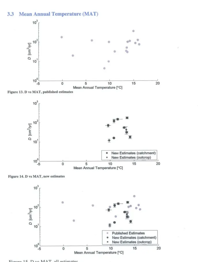
The new and existing soil transport coefficient estimates are shown here plotted against the mean annual precipitation (Figure 7-Figure 9), aridity index (Figure 10-Figure 12), and mean annual temperature (Figure 13-Figure 15). The data for these plots are summarized in Table 1, and a full table with data for individual measurements made is included in the Appendix 7.2 (Table 2). Numbered versions of Figure 9 and Figure 12 with individual sites identified are presented as Figure 16 and Figure 17, respectively, in

Appendix 7.1.

Error bars have been included on the new measurements to show one standard error of the mean in both directions, reflecting uncertainty in estimates of D and climate for sites where multiple erosion rate estimates and ridgelines were used to create the site estimate.

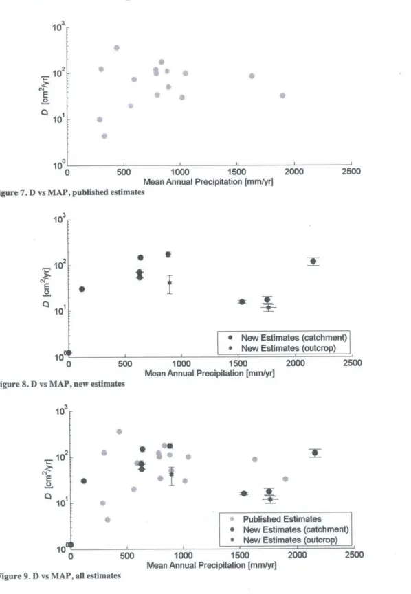
There appears to be an upward trend in both the published and new values of D versus MAP in the precipitation range from 0 mm/yr to 1000 mm/yr (Figure 7). The new estimates show a slightly downward trend from 600 to 1600 mm/yr (Figure 8), but the downturn is not as well-defined, especially when viewed in conjunction with the

published data. Together, the published and new estimates suggest a relationship in which D rises with precipitation for low MAP and either decreases gradually or stays approximately constant with precipitation for higher MAP (Figure 9).

Similar trends are visible in the data for D versus Al (Figure 10-Figure 12), in which there is an upward trend in D for low Al (drier climates) that levels off or gradually decreases for higher Al (wetter climates).

(24)

The Oregon Coast Range, which has both the highest mean annual precipitation and aridity index, appears as an outlier.

(25)

3.1 Mean Annual Precipitation (MAP)

Tr E 1o2 101 1001 0 500

Figure 7. D vs MAP, published estimates

E 102 101 100 0 1000 1500

Mean Annual Precipitation [mm/yr]

0

t

2000

* New Estimates (catchment)

* New Estimates (outcrop)

I I I

500 1000 1500

Mean Annual Precipitation [mm/yr]

2000 Figure 8. D vs MAP, new estimates

C4 E 102 101 10 0

Figure 9. D vs MAP, all estimates

0

*

_I:f

*

Published Estimates New Estimates (catchment) New Estimates (outcrop)

i00 1000 1500

Mean Annual Precipitation [mm/yr]

2000 2500

2500

::C

(26)

3.2 Aridity Index (AI)

103 E 102 10 10 0 0.5 1 1.5 Aridity Index 2 2.5 3

Figure 10. D vs Al, published estimates

E 0 102 101 10 0 0

-v

#.

9.0

* New Estimates (outcrop)

0.5 1 1.5

Aridity Index

2 2.5 3

Figure 11. D vs Al, new estimates

0

9.

*

1

Published Estimates New Estimates (catchment) New Estimates (outcrop)

0.5 1 1.5

Aridity Index

2 2.5 3

Figure 12. D vs AI, all estimates

'U 102 101 E 0 10 0

I

--- L-0

(27)

3.3 Mean Annual Temperature (MAT)

E 0 102 101 100L -5 0

Figure 13. D vs MAT, published estimates

103 E 102 10 -5 5 10

Mean Annual Temperature [*C]

15 20

* New Estimates (outcrop) I

0 5 10

Mean Annual Temperature [*C]

15 20

Figure 14. D vs MAT, new estimates

10 102 10 E 10o -5 Published Estimates * New Estimates (catchment) * New Estimates (outcrop)

0 5 10

Mean Annual Temperature (*CJ

15 20

(28)

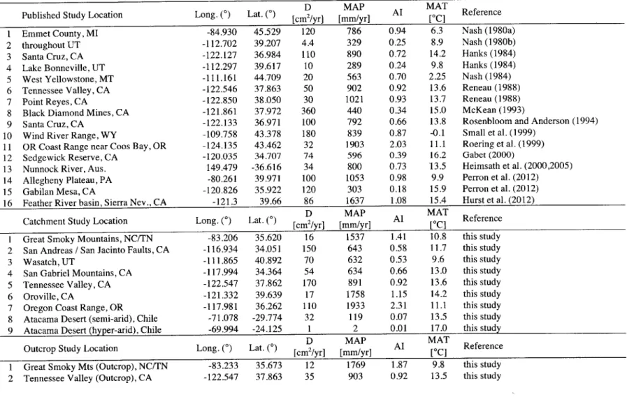
Table 1. Summary of Results

D MAP MAT

Published Study Location Long. (*) Lat. (0) [cm2/yr] [mmyr] Al [C] Reference

1 Emmet County, MI -84.930 45.529 120 786 0.94 6.3 Nash (1980a)

2 throughout UT -112.702 39.207 4.4 329 0.25 8.9 Nash (1980b)

3 Santa Cruz, CA -122.127 36.984 110 890 0.72 14.2 Hanks(1984)

4 Lake Bonneville, UT -112.297 39.617 10 289 0.24 9.8 Hanks(1984)

5 West Yellowstone, MT -111.161 44.709 20 563 0.70 2.25 Nash (1984)

6 Tennessee Valley, CA -122.546 37.863 50 902 0.92 13.6 Reneau (1988)

7 Point Reyes, CA -122.850 38.050 30 1021 0.93 13.7 Reneau (1988)

8 Black Diamond Mines, CA -121.861 37.972 360 440 0.34 15.0 McKean (1993)

9 Santa Cruz, CA -122.133 36.971 100 792 0.66 13.8 Rosenbloom and Anderson (1994)

10 Wind River Range, WY -109.758 43.378 180 839 0.87 -0.1 Small et al. (1999)

11 OR Coast Range near Coos Bay, OR -124.135 43.462 32 1903 2.03 11.1 Roering et al. (1999)

12 Sedgewick Reserve, CA -120.035 34.707 74 596 0.39 16.2 Gabet (2000)

13 Nunnock River, Aus. 149.479 -36.616 34 800 0.73 13.5 Heimsath et al. (2000,2005)

14 Allegheny Plateau, PA -80.261 39.971 100 1053 0.98 9.9 Perron et al. (2012)

15 Gabilan Mesa, CA -120.826 35.922 120 303 0.18 15.9 Perron et al. (2012)

16 Feather River basin, Sierra Nev., CA -121.3 39.66 86 1637 1.08 15.4 Hurst et al. (2012)

D MAP MAT

Catchment Study Location Long. () Lat. () [cm2/yr] [mm/yr] Al [C Reference

1 Great Smoky Mountains, NC/TN -83.206 35.620 16 1537 1.41 10.8 this study

2 San Andreas / San Jacinto Faults, CA -116.934 34.051 150 643 0.58 11.7 this study

3 Wasatch, UT -111.865 40.892 70 632 0.53 9.6 this study

4 San Gabriel Mountains, CA -117.994 34.364 54 634 0.66 13.0 this study

5 Tennessee Valley, CA -122.547 37.862 170 891 0.92 13.6 this study

6 Oroville, CA -121.332 39.639 17 1758 1.15 14.2 this study

7 Oregon Coast Range, OR -117.981 36.262 110 1933 2.31 11.1 this study

8 Atacama Desert (semi-arid), Chile -71.078 -29.774 32 119 0.07 13.5 this study

9 Atacama Desert (hyper-arid), Chile -69.994 -24.125 1 2 0.01 17.0 this study

D MAP MAT

Outcrop Study Location Long. (0) Lat. (0) [cm2/yr] [mm/yr] Al [oC] Reference

1 Great Smoky Mts (Outcrop), NC/TN -83.233 35.673 12 1769 1.87 9.8 this study

(29)

4 Discussion

Both the D versus MAP and D versus Al plots suggest a relationship between D and wetness in which D increases steeply with MAP and Al in drier climates, and

decreases gradually with MAP and Al in wetter climates. The peak D appears to occur at an MAP of approximately 500-1000 mm/yr and an Al of approximately 0.5-1.

The upward trend for low MAP and Al is in agreement with the prediction by

Owen et al. [2011]. In very dry climates, there is little biota to agitate the soil. The

semiarid Atacama site with 120 mm/yr had a plant density of 30%, while the hyper-arid Atacama site with a MAP of less than 2 mm/yr had a plant density of 0. The landscape at the semi-arid site undergoes bioturbation and chemical weathering processes while the

landscape at the hyper-arid site is too dry for bioturbation and is acted upon primarily by salt shrink-swell and overland flow, which are less effective at transporting soil. Thus it seems that the climate is affecting the soil transport efficiency through the biota that it supports.

The lack of a trend in D versus MAT is not surprising for this range of

temperatures. The new sites in particular have a very limited MAT range where biotic factors are not expected to be reflected. Even with the published data, which has a larger MAT range, the lower end where cold-dependent abiotic processes are expected to be more effective is not well represented.

4.1 General Observations

With the exception of the Oregon Coast Range, the new D estimates show a cleaner trend than the published values in both MAP and Al. Consistency in the

(30)

estimation method for the new D values may be contributing to the cleaner trend in the new data, but additional estimates in overlapping climate ranges would need to be compared to see whether this holds in general.

The assumptions that the landscape is in steady state, that linear transport applies, and that modern climate is representative of the climate in which the landscapes formed

are also potential sources of uncertainty. The steady state assumption was tested qualitatively by the area-slope product plot created as part of the Method, and the linear slope dependence is approximated by applying the analysis only on ridgelines. The climate assumption is more challenging. The timescale for hillslope evolution depends on D, but is typically on the order of 105~106 years [Fernandes and Dietrich, 1997],

which is at least as long as a glacial cycle.

One note is that in adding 9 new estimates to the data set over a range of climates, the range of D remains relatively unchanged since Fernandes and Dietrich [1997] noted that existing estimates of D ranged from 4 to 400 cm2/yr. Estimates in the Atacama Desert added a new low D of 1 cm2/yr, but the upper bound of 360 cm2/yr [McKean, et

al., 1993] was not exceeded.

4.2 Specific Site Notes

The estimate presented here for Tennessee Valley is much higher than the existing estimate presented by Reneau [1988], whose estimate is based on the infilling of a dated landslide scar. The topographical curvature method used here is considered to be more

precise, but further investigation is required.

The Great Smoky Mountains have a lower D than anticipated in comparison to D calculated for the Allegheny Plateau [Perron et al., 2012], which is also in the

(31)

Appalachian Mountains. The ridgetops at the Great Smoky Mountains site are relatively sharp and the erosion rates are very low, which results in a low estimate for D.

The site used for the Oregon Coast Range measurement in this study is located in the northern tip of the Siuslaw National Forest, approximately 150 km north of Coos Bay,

where Roering et al. [1999] estimated D to be 32 cm2/yr. The reason why the D value estimated in this study (110 cm2

/yr) is so high is currently unclear, and the measurement at the Oregon Coast Range site will be re-examined. There is, however, a large

variability in erosion rates at this site. Three samples within 500 m of each other have bedrock erosion rates of 66, 138, and 300 mm/kyr, which suggests that the erosion rate is not well-constrained for this site.

The estimate for Oroville, which is at the Feather River site studied by Riebe et al. [2000], is much lower than the estimate presented by Hurst et al. [2012] for the same site.

Hurst et al. used the slope of a Laplacian versus erosion rate trend line over 25 hillslopes

to estimate D for the region as a whole. The estimate presented in this study used only one hillslope, so it is not unsurprising that it does not match the prediction by Hurst et al. Performing this analysis on a subset of the hillslopes used by Hurst et al. will give a better idea of the compatibility of the results.

4.3 Other Factors and Future Work

While several factors have been identified as influencing D (Section 1.2), this work focused solely on annual climate proxies. As such, this work does not attempt to account for differences in D caused by differences in rock and soil type or grain size, which was used to explain variations in D by McKean et al. [1993]. The sites presented here could be classified by bedrock type to determine whether an effect is visible.

(32)

This study also does not track biota directly. In the indirect sense, MAP and Al affect the populations that a region can support, but this relationship is not explored quantitatively here.

By using annually averaged climate proxies, seasonality and higher-frequency variations are not considered. Two sites with similar MAP may experience different soil transport processes if one site has distinct wet and dry seasons and the other does not, just

as two sites with similar MAT may experience different soil transport processes if one has temperatures that vary significantly over the course of a day or a year while the other

has less variation. Interpreting the D values presented here in terms of seasonality may provide further insight.

In addition to including seasonality, understanding of the potential relationship between D and climate could be improved by considering sites with even higher MAP, and by making comparisons of D across a smaller region that still varies significantly in

MAP.

While the new sites analyzed here extended the MAP values through the 0-300 and 1000-2300 mm/yr range, a lack of data remains for the high precipitation values above 2300 mm/yr. Erosion rate estimates have been made for basins in northern Kauai near Hanalei Bay [Ferrier et al., 2013ab] (K. Huppert and K. Ferrier, personal

communication, 2014) and in Luquillo, Puerto Rico, both of which have MAP of approximately 3000 mm/yr. LIDAR also exists for both sites, though the ground return for Luquillo is sparse due to dense vegetation. The value of D is expected to be low for the Hanalei sites since the ridgelines are sharp and the estimated erosion rates are not unusually fast.

(33)

Kauai alone has a wide range of MAP (700 to 7000 mm/yr) at sites where erosion rate estimates have been made. Estimating D at various sites that have soil-mantled landscapes and seeing whether the relationship holds throughout Kauai alone would likely be informative.

(34)

5 Conclusions

This work presents new estimates of the soil transport coefficient D at 9 sites and compares them, along with a compilation of 16 previously published estimates of D, against three climate proxies (mean annual precipitation, aridity index, and mean annual temperature) with the goal of characterizing climatic influences on soil transport

efficiency. The previously published data was primarily clustered at sites with MAP of 300 to 1000 mm/yr, while the new measurements were performed at sites that extend the range into both drier and wetter climates.

The results show no relationship between D and mean annual temperature. However, the results do suggest a relationship between D and "wetness" measured by both the mean annual precipitation (MAP) and the aridity index (Al). At low MAP and Al, D steeply increases with these climate proxies, and at higher MAP and Al, D

decreases gently with these climate proxies. The peak occurs near MAP values of 500 and 1000 mm/yr, and Al values of 0.5 and 1. This is consistent with ideas proposed by

Owen et al. [2011 ] and Perron et al. [2009].

Not all sites in the compilation follow this trend. In particular, the new estimate for the Oregon Coast Range departs from the downward trend of the other data with

MAP above 600 mm/yr. Verifying the quality of the new estimates, particularly at sites with over 1000 mm/yr, and adding data at sites with high MAP (above 2500mm/yr) should better constrain the behavior in wetter climates.

While the relationship is not yet quantifiable, and the data is not complete for the higher ranges of MAP and AI, the data presented here leads to the conclusion that climate

(35)

better clarify a relationship between D and climate that would allow for improvements in landscape evolution modeling and the understanding of the ties between landscape and the climate in which it forms.

(36)

6 References

Balco, G., J. 0. Stone, N. A. Lifton, and T. J. Dunai (2008), A complete and easily accessible means of calculating surface exposure ages or erosion rates from ' Be and 26Al measurements. Quat. Geochronol. 3, 174-195.

Culling, W.E.H., (1960) Analytical theory of erosion, J. Geol., 68, 336- 344.

DiBiase, R. A., K. X. Whipple, A. M. Heimsath, and W. B. Ouimet (2010) Landscape

form and millennial erosion rates in the San Gabriel Mountains, CA, Earth and Planetary Science Letters, 289, 134-144.

Dietrich, W. E., Bellugi, D. G., Sklar, L. S., Stock, J. D., Heimsath, A. M. and Roering, J.

J. (2003) Geomorphic Transport Laws for Predicting Landscape form and Dynamics, in Prediction in Geomorphology (eds P. R. Wilcock and R. M. Iverson), American

Geophysical Union, Washington, D. C.. doi: 10.1029/135GM09

Fernandes, N. F., and W. E. Dietrich (1997) Hillslope evolution by diffusive processes: The timescale for equilibrium adjustments, Water Resources Research, 33(6), 1307-1318. Ferrier, K. L., K. L. Huppert, and J. T. Perron (2013), Evidence for climatic control of bedrock river incision. Nature, 496, 206-209, doi:10.1038/nature11982.

Ferrier, K. L, J. T. Perron, S. Mukhopadhyay, M. Rosener, J. D. Stock, K. L. Huppert,

and M. Slosberg (2013), Covariation of climate and long-term erosion rates across a steep

rainfall gradient on the Hawaiian island of Kaua'i. GSA Bulletin, doi: 10.11 30/B 30726.1.

Gabet, M. J. (2000) Gopher bioturbation: field evidence for non-linear hillslope diffusion,

Earth Surf. Process. Landforms, 25, 1419-1428.

Hanks, T. C., Bucknam, R. C., Lajoie, K. R., and Wallace, R. E. (1984) Modification of

Wave-Cut and Faulting-Controlled Landforms, Journal of Geophysical Research, 89(B7), 5571-5590.

Howard, A. D. (1994) A detachment-limited model of drainage basin evolution. Wat. Resour. Res. 30, 2261-2286.

Hurst, M. D., S. M. Mudd, R. Walcott, M. Attal, and K. Yoo (2012), Journal of Geophysical Research, 117, F02017, doi: 10.1029/2011JF002057.

Matmon, A., P. R. Bierman, J. Larsen, S. Southworth, M. Pavich, R. Finkel, and M. Caffee (2003) Erosion of an ancient mountain range, the Great Smoky Mountains, North

(37)

McKean, J. A., W. E. Dietrich, R. C. Finkel, J. R. Southon, M. W. Caffee (1993)

Quantification of soil production and downslope creep rates from cosmogenic 'OBE accumulations on a hillslope profile, Geology, 21, 343-346.

Nash, D. (1980) Forms of bluffs degraded for different lengths of time in Emmet County,

Michigan, U.S.A., Earth Surface Processes, 5, 331-345.

Nash, D. B. (1980) Morphologic Dating of Degraded Normal Fault Scarps, The Journal of Geology, 88(3), 353-360.

Nash, D. B. (1984) Morphologic dating of fluvial terrace scarps and fault scarps near West Yellowstone, Montana, Geological Society of America Bulletin, 95, 1413-1424. Owen, J. J, R. Amundson, W. E. Dietrich, K. Nishiizumi, B. Sutter, and G. Chong (2011) The sensitivity of hillslope bedrock erosion to precipitation, Earth Surf. Process.

Landforms, 36, 117-135, doi: 10.1002/esp.2083.

Perron, J. T., J. W. Kirchner, W. E. Dietrich (2009), Formation of evenly spaced ridges

and valleys, Nature, 460(7254), 502-505, doi: 10.1038/nature08174.

Perron, J. T., P. W. Richardson, K. L. Ferrier, and M. Lap6tre (2012). The root of branching river networks, Nature, 492, 100-103, doi:10.1038/nature 11672.

Portenga, E. W., and P. R. Bierman (2011), Understanding Earth's eroding surface with

'0Be, GSA Today, 21(8), doi: 10.1130/G 111A.1.

Portenga, E. W., and P. R. Bierman (2011), GSA supplemental data item 2011216, www.geosociety.org/pubs/ft20 11.htm.

Riebe, C. S., J. W. Kirchner, D. E. Granger, and R. C. Finkel (2000), Erosional

equilibrium and disequilibrium in the Sierra Nevada, inferred from cosmogenic 26AI and '0Be in alluvial sediment, Geology 28(9), 803-806. Supplement Data Repository item

200084.

Riebe, C. S., J. W. Kirchner, D. E. Granger, and R. C. Finkel (2001), Minimal climatic control on erosion rates in the Sierra Nevada, California, Geology 29(5), 447-450. Roering, J. J., J. W. Kirchner, and W. E. Dietrich (1999), Evidence for nonlinear, diffusive sediment transport on hillslopes and implications for landscape morphology,

Wat. Resour. Res. 35(3), 853-870.

Rosenbloom, N. A., and R. S. Anderson (1994), Hillslope and channel evolution in a marine terraced landscape, Santa Cruz, California, Journal of Geophysical Research, 99(B7), 14013-14029.

(38)

Small, E. E., R. S. Anderson, and G. S. Hancock (1999), Estimates of the rate of regolith production using ' Be and 26

Al from an alpine hillslope, Geomorphology, 27, 131-150. Tucker, G. E. and R. L. Bras (1998) Hillslope processes, drainage density, and landscape

morphology. Wat. Resour. Res. 34, 2751-2764.

Willenbring, J. K., A. T. Codilean, B. McElroy (2013) Earth is (mostly) flat:

Apportionment of the flux of continental sediment over millennial time scales.

Supplement. GSA data repository 2013091.

Willenbring, J. K., A. T. Codilean, B. McElroy (2013) Earth is (mostly) flat:

Apportionment of the flux of continental sediment over millennial time scales, Geology,

42(1),e316,doi: 10.1130/G34846C..

Willgoose, G., R. L. Bras, and I. Rodriguez-Iturbe (1991), Results from a new model of river basin evolution. Earth Surf. Process. Landf. 16, 237-254.

Zomer R. J., A. Trabucco, D. A. Bossio, 0. van Straaten, and L. V. Verchot (2008),

Climate Change Mitigation: A Spatial Analysis of Global Land Suitability for Clean

Development Mechanism Afforestation and Reforestation. Agric. Ecosystems and Envir. 126,67-80.

Zomer, R. J., D. A. Bossio, A. Trabucco, L. Yuanjie, D. C. Gupta and V. P. Singh (2007),

Trees and Water: Smallholder Agroforestry on Irrigated Lands in Northern India.

Colombo, Sri Lanka: International Water Management Institute, IWMI Research Report, 122,45.

(39)

7 Appendix

Appendix Contents:

7.1 Selected plots with site identification 7.2 Individual measurement summary 7.3 Sample features to mask from DEM 7.4 Analysis output images

This section contains satellite views, hillshades, Laplacian maps, Laplacian vs area-slope product plots, and ridgeline selection map for each site at which calculations were made.

(40)

7.1 Selected plots with site identification

10I 102 E5 101 10.5 '15 *14 1& -,13 .9 -16 .6 .11 *1

10 --

r

I 0 500 10 1500

Mean Annual Precipitation [mm/yr]

Published Estimates New Estimates (catchment) * New Estimates (outcrop)

2000 2500

Published Study Location

1 Emmet County, MI, Nash (1980a)

2 throughout UT, Nash (1980b) 3 Santa Cruz, CA, Hanks (1984) 4 Lake Bonneville, UT, Hanks (1984) 5 West Yellowstone, MT, Nash (1984) 6 Tennessee Valley, CA, Reneau (1988) 7 Point Reyes, CA, Reneau (1988)

8 Black Diamond Mines, CA, McKean (1993)

9 10 I1 12 13 14 15 16

Published Study Location

Santa Cruz, CA, Rosenbloom and Anderson (1994)

Wind River Range, WY, Small et al. (1999) Coast Range near Coos Bay, OR, Roering et al. (1999)

Sedgewick Reserve, CA, Gabet (2000)

Nunnock River, Aus., Heimsath et al. (2000,2005) Allegheny Plateau, PA, Perron et al. (2012) Gabilan Mesa, CA, Perron et al. (2012)

Feather River, Sierra Nev., CA, Hurst et al. (2012)

1 2 3 4 5 6 7 8

Figure 16. D vs MAP with sites identified

Catchment Study Location

Great Smoky Mountains, NC/TN

San Andreas / San Jacinto Faults, CA

Wasatch, UT

San Gabriel Mountains, CA

Tennessee Valley, CA

Oroville, CA

Oregon Coast Range, OR Atacama Desert (semi-arid), Chile

Catchment Study Location

8 Atacama Desert (semi-arid), Chile

9 Atacama Desert (hyper-arid), Chile

Outcrop Study Location

I Great Smoky Mts (Outcrop), NC/TN

2 Tennessee Valley (Outcrop), CA

'1 .9

(41)

102 Q 10 1000 015 5512 3 10 gi416 .4 $8 .2 q,13 _Z _9 .1 .7 11 *1 Published Estimates * New Estimates (catchment)

* New Estimates (outcrop)

0.5 1.5 2

Aridity Index

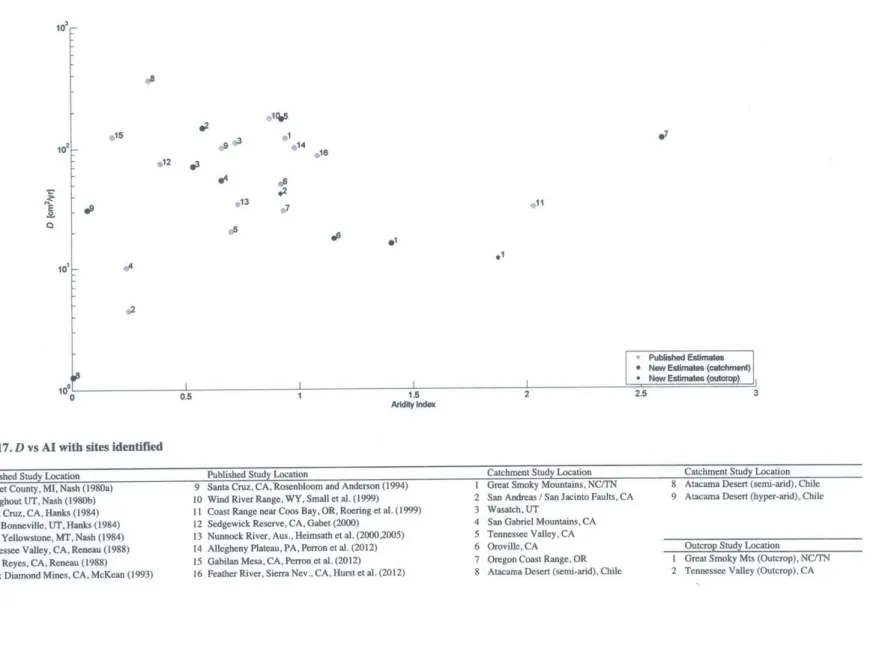
Figure 17. D vs Al with sites identified

Published Study Location Published Study Location Catchment Study Location Catchment Study Location

I Emmet County, MI, Nash (1980a) 9 Santa Cruz, CA,'Rosenbloom and Anderson (1994) 1 Great Smoky Mountains, NC/TN 8 Atacama Desert (semi-arid), Chile

2 U . UT Mah (loe8i 10 Wind River Range WY Small et al. (1999) 2 San Andreas / San Jacinto Faults, CA 9 Atacama Desert (hyper-arid), Chile

troug 0u

,

Santa Cruz, CA, Hanks (1984) Lake Bonneville, UT, Hanks (1984)

West Yellowstone, MT, Nash (1984) Tennessee Valley, CA, Reneau (1988) Point Reyes, CA, Reneau (1988) Black Diamond Mines, CA, McKean (1993)

11 12 13 14 15 16 , ,I

Coast Range near Coos Bay, OR, Roering et al. (1999)

Sedgewick Reserve, CA, Gabet (2000) Nunnock River, Aus., Heimsath et al. (2000,2005) Allegheny Plateau, PA, Perron et al. (2012) Gabilan Mesa, CA, Perron et al. (2012)

Feather River, Sierra Nev., CA, Hurst et al. (2012)

3 4 5 6 7 8 Wasatch, UT

San Gabriel Mountains, CA Tennessee Valley, CA

Oroville, CA Oregon Coast Range, OR Atacama Desert (semi-arid), Chile

Outcrop Study Location

I Great Smoky Mts (Outcrop), NC/TN 2 Tennessee Valley (Outcrop), CA

3 4 5 6 7 8

39

0 3 1 2 2.5

(42)

7.2 Individual measurement summary

Table 2. Extended table showing individual measurement data

Site Location Long.(0) Lat.(0) D MAP AI MAT V2

z U Pb/P, Compilation

no. [cm2/yr] [mm/yr] [

0

C] [m1] [m/Myr] ID*

1 Great Smoky Mountains, NC/TN -83.193 35.629 15 1600 1.466 10.6 -0.0288 26.34 2.7/1.6 GSRF-2P,

WTS10002

1 Great Smoky Mountains, NC/TN -83.194 35.629 11 1600 1.343 10.6 -0.0288 19.52 2.7/1.6 GSRF-3 P

1 Great Smoky Mountains, NC/TN -83.199 35.623 16 1540 1.381 11.0 -0.0288 27.28 2.7/1.6 GSRF-5 P

1 Great Smoky Mountains, NC/TN -83.2117 35.622 17 1520 1.317 11.0 -0.0288 28.64 2.7/1.6 GSRF-6 P,

I I WTS10005

1 Great Smoky Mountains, NC/TN -83.2081 35.618 14 1500 1.379 10.8 -0.0288 23.40 2.7/1.6 GSRF-7 ,

WTS10006

1 Great Smoky Mountains, NC/TN -83.2133 35.613 18 1500 1.466 10.8 -0.0288 31.49 2.7/1.6 GSRF-8 P,

WTS10007

1 Great Smoky Mountains, NC/TN -83.2243 35.608 19 1500 1.487 10.9 -0.0288 31.92 2.7/1.6 GSRF-9 ,

WTS10008

2 San Andreas / San Jacinto Faults, -116.928 34.050 160 660 0.560 10.7 -0.1507 1460.72 2.7/1.6 WTS26003

CA

2 San Andreas / San Jacinto Faults, -116.9401 34.053 130 630 0.593 12.6 -0.1645 1284.58 2.7/1.6 WTS26004

CA 3 Wasatch, UT -111.9012 41.107 58 756 0.568 8.1 -0.0210 71.81 2.7/1.6 KC', WTS39001 3 Wasatch, UT -111.8713 40.976 65 590 0.560 10.6 -0.0201 77.87 2.7/1.6 StC', WTS39005 3 Wasatch, UT -111.8698 40.934 110 610 0.463 10.0 -0.0168 113.08 2.7/1.6 FCP, WTS39006 3 Wasatch, UT -111.8627 40.917 77 570 0.491 10.9 -0.0160 72.83 2.7/1.6 CC", WTS39007 3 Wasatch, UT -111.819 40.521 38 630 0.592 8.5 -0.0496 110.97 2.7/1.6 BC", WTS39015

4 San Gabriel Mountains, CA -117.992 34.367 58 600 0.658 13.3 -0.0302 107.77 2.7/1.6 SG131",

I_ WTS40023

(43)

4 San Gabriel Mountains, CA -117.996 34.362 50 670 0.658 12.7 -0.0411 126.19 2.7/1.6 SG205 ,

WTS40040

5 Tennessee Valley, CA -122.546 37.863 160 910 0.924 13.4 -0.0102 79.20 2.8/1.4 creek1

5 Tennessee Valley, CA -122.548 37.861 190 880 0.924 13.8 -0.0130 125.30 2.8/1.4 creek2

6 Oroville, CA -121.332 39.639 21 1760 1.154 14.2 -0.0208 28.05 2.7/1.6 FR-6 P

6 Oroville, CA -121.331 39.639 14 1760 1.154 14.2 -0.0208 19.61 2.7/1.6 FR-7 P

7 Oregon Coast Range, OR -123.852 44.537 64 2130 2.629 10.8 -0.0252 113.11 2.7/1.6 dc-29 ,

WTS55007

7 Oregon Coast Range, OR -123.867 44.524 110 2210 2.642 10.8 -0.0232 180.98 2.7/1.6 dc-30,

WTS55008

7 Oregon Coast Range, OR -123.859 44.509 59 2160 2.595 10.9 -0.0160 65.82 2.7/1.6 dc-31] ,

WTS55009

7 Oregon Coast Range, OR -123.818 44.519 100 2160 2.561 10.9 -0.0191 137.75 2.7/1.6 dc-35 ,

WTS55010

7 Oregon Coast Range, OR -123.818 44.516 110 2160 2.589 10.9 -0.0191 153.56 2.7/1.6 dc-36P,

WTS55011

7 Oregon Coast Range, OR -123.821 44.514 110 2140 2.589 10.8 -0.0191 146.44 2.7/1.6 dc-37p,

WTS55012

7 Oregon Coast Range, OR -123.854 44.508 120 2160 2.583 10.9 -0.0160 138.31 2.7/1.6 dc-38 ,

WTS55013

7 Oregon Coast Range, OR -123.859 44.507 270 2160 2.556 10.9 -0.0160 300.41 2.7/1.6 dc-40,

WTS55014

8 Atacama Desert (semi-arid), Chile -71.078 -29.774 23 120 0.070 13.5 -0.0159 20 2.7/1.35 SGA-1

8 Atacama Desert (semi-arid), Chile -71.078 -29.774 40 120 0.070 13.5 -0.0159 35 2.7/1.4 SGA-4

8 Atacama Desert (semi-arid), Chile -71.078 -29.774 32 120 0.070 13.5 -0.0159 28 2.7/1.5 SGA-06-28

8 Atacama Desert (semi-arid), Chile -71.078 -29.774 25 120 0.070 13.5 -0.0159 22 2.7/1.51 SGA-06-17

8 Atacama Desert (semi-arid), Chile -71.078 -29.774 20 120 0.070 13.5 -0.0159 17 2.7/1.49 SGA-06-16

8 Atacama Desert (semi-arid), Chile -71.078 -29.774 39 120 0.070 13.5 -0.0159 34 2.7/1.6 SGA05-14b

9 Atacama Desert (hyper-arid), Chile -69.994 -24.125 1.1 2 0.005 17.0 -0.0302 0.95 2.7/0.8 YH-05-16c