HAL Id: hal-03009572
https://hal.archives-ouvertes.fr/hal-03009572
Submitted on 19 Nov 2020
HAL is a multi-disciplinary open access
archive for the deposit and dissemination of
sci-entific research documents, whether they are
pub-lished or not. The documents may come from
teaching and research institutions in France or
abroad, or from public or private research centers.
L’archive ouverte pluridisciplinaire HAL, est
destinée au dépôt et à la diffusion de documents
scientifiques de niveau recherche, publiés ou non,
émanant des établissements d’enseignement et de
recherche français ou étrangers, des laboratoires
publics ou privés.
the Hot Jupiter WASP-43b and Predictions for JWST
Olivia Venot, Vivien Parmentier, Jasmina Blecic, Patricio Cubillos, Ingo
Waldmann, Quentin Changeat, Julianne Moses, Pascal Tremblin, Nicolas
Crouzet, Peter Gao, et al.
To cite this version:
Olivia Venot, Vivien Parmentier, Jasmina Blecic, Patricio Cubillos, Ingo Waldmann, et al.. Global
Chemistry and Thermal Structure Models for the Hot Jupiter WASP-43b and Predictions for JWST.
The Astrophysical Journal, American Astronomical Society, 2020, 890 (2), pp.176.
�10.3847/1538-4357/ab6a94�. �hal-03009572�
TEX twocolumn style in AASTeX61
GLOBAL CHEMISTRY AND THERMAL STRUCTURE MODELS FOR THE HOT JUPITER WASP-43b AND PREDICTIONS FOR JWST
OLIVIAVENOT,1VIVIENPARMENTIER,2JASMINABLECIC,3PATRICIOE. CUBILLOS,4INGOP. WALDMANN,5QUENTINCHANGEAT,5
JULIANNEI. MOSES,6PASCALTREMBLIN,7NICOLASCROUZET,8 PETERGAO,9DIANAPOWELL,10PIERRE-OLIVIERLAGAGE,11
IANDOBBS-DIXON,3MARIAE. STEINRUECK,12LAURAKREIDBERG,13, 14NATALIEBATALHA,15JACOBL. BEAN,16
KEVINB. STEVENSON,17S
ARAHCASEWELL,18
ANDLUDMILACARONE19
1Laboratoire Interuniversitaire des Systèmes Atmosphériques (LISA), UMR CNRS 7583, Université Paris-Est-Créteil, Université de Paris, Institut Pierre Simon
Laplace, Créteil, France
2AOPP, Department of Physics, University of Oxford 3NYU Abu Dhabi, Abu Dhabi, UAE
4Space Research Institute, Austrian Academy of Sciences, Schmiedlstr. 6, 8042, Graz, Austria
5University College London, Department of Physics and Astronomy, Gower Street, London WC1E 6BT, UK 6Space Science Institute, Boulder, CO, USA
7Maison de la Simulation, CEA, CNRS, Univ. Paris-Sud, UVSQ, Université Paris-Saclay, 91191 Gif-sur-Yvette, France
8Science Support Office, Directorate of Science, European Space Research and Technology Centre (ESA/ESTEC), Keplerlaan 1, 2201 AZ Noordwijk, The
Netherlands
9Astronomy Department, University of California, Berkeley, 501 Campbell Hall, MC 3411, Berkeley, CA 94720 10Department of Astronomy and Astrophysics, University of California, Santa Cruz, CA 95064, USA
11AIM, CEA, CNRS, Université Paris-Saclay, Université Paris Diderot, Sorbonne Paris Cité, UMR7158 F-91191 Gif-sur-Yvette, France 12Lunar and Planetary Laboratory, University of Arizona, 1629 E University Blvd, Tucson, AZ 85719, USA
13Harvard-Smithsonian Center for Astrophysics, 60 Garden Street, Cambridge, MA 02138 14Harvard Society of Fellows, 78 Mount Auburn Street, Cambridge, MA 02138
15Department of Astronomy & Astrophysics, University of California, Santa Cruz, CA 95064, USA
16Department of Astronomy & Astrophysics, University of Chicago, 5640 S., Ellis Avenue, Chicago, IL 60637, USA 17Space Telescope Science Institute, 3700 San Martin Drive, Baltimore, MD 21218, USA
18Dept. of Physics and Astronomy, Leicester Institute of Space and Earth Observation, University of Leicester, University Road,Leicester, LE1 7RH, UK 19Max Planck Institute for Astronomy, Koenigsstuhl 17, D-69117 Heidelberg, Germany
ABSTRACT
The James Webb Space Telescope (JWST) is expected to revolutionize the field of exoplanets. The broad wavelength coverage and the high sensitivity of its instruments will allow characterization of exoplanetary atmospheres with unprecedented precision. Following the Call for the Cycle 1 Early Release Science Program, the Transiting Exoplanet Community was awarded time to observe several targets, including WASP-43b. The atmosphere of this hot Jupiter has been intensively observed but still harbors some mysteries, especially concerning the day-night temperature gradient, the efficiency of the atmospheric circulation, and the presence of nightside clouds. We will constrain these properties by observing a full orbit of the planet and extracting its spectroscopic phase curve in the 5–12 µm range with JWST/MIRI. To prepare for these observations, we performed an extensive modeling work with various codes: radiative transfer, chemical kinetics, cloud microphysics, global circulation models, JWST simulators, and spectral retrieval. Our JWST simulations show that we should achieve a precision of 210 ppm per 0.1 µm spectral bin on average, which will allow us to measure the variations of the spectrum in longitude and measure the night-side emission spectrum for the first time. If the atmosphere of WASP-43b is clear, our observations will permit us to determine if its atmosphere has an equilibrium or disequilibrium chemical composition, providing eventually the first conclusive evidence of chemical quenching in a hot Jupiter atmosphere. If the atmosphere is cloudy, a careful retrieval analysis will allow us to identify the cloud composition.
Keywords:methods: numerical — planets and satellites: atmospheres — planets and satellites: composition — planets and satellites: gaseous planets — planets and satellites: individual (WASP-43b) — tech-niques: spectroscopic
1. INTRODUCTION
Giant planets that orbit very close to their host stars — so-called “hot Jupiters” — are expected to be tidally locked, with one hemisphere constantly facing the star, and one hemisphere in perpetual darkness. The uneven stellar irra-diation incident on such planets leads to strong and unusual radiative forcing, resulting in large temperature gradients and complicated atmospheric dynamics. The atmospheric com-position and cloud structure on these planets can, in turn, vary in three dimensions as the temperatures change across the globe, and as winds transport constituents from place to place. Strong couplings and feedbacks between atmospheric chemistry, cloud formation, radiative transfer, energy trans-port, and atmospheric dynamics exist to further influence atmospheric properties. The inherently non-uniform nature of these atmospheres complicates derivations of atmospheric properties from transit, eclipse, and phase curve observa-tions. Three-dimensional models that can track the relevant physics and chemistry on all scales — both large and small distance scales, and large and small time scales — are needed to accurately interpret hot Jupiter spectra.
Discovered in 2011 byHellier et al.(2011), the hot Jupiter WASP-43b orbits a relatively cool K7V star (4 520 ± 120 K,Gillon et al. 20121). It has the smallest semi-major axis
of all confirmed hot Jupiters and one of the shortest orbital periods (0.01526 AU and 19.5 h respectively, Gillon et al. 2012). In addition to its exceptionally short orbit, WASP-43b is very good candidate for in-depth atmospheric charac-terization through transit thanks to its large planet-star radius ratio and the brightness of its host star, leading to a very good signal-to-noise ratio. The planet is also a good candidate for eclipse and phase curve observations thanks to the important flux ratio between the emission of the star and the exoplanet. To date, many observations of the planet’s atmosphere have been conducted from the ground (Gillon et al. 2012;
Wang et al. 2013; Chen et al. 2014; Murgas et al. 2014;
Zhou et al. 2014; Jiang et al. 2016; Hoyer et al. 2016) and from space (Blecic et al. 2014; Kreidberg et al. 2014;
Stevenson et al. 2014, 2017; Ricci et al. 2015). Most no-tably, orbital phase curves have been observed with both the Hubble Space Telescope (HST) from 1.1 to 1.7µm ( Steven-son et al. 2014) and with the Spitzer Space Telescope at 3.6µm and 4.5µm (Stevenson et al. 2016). Whereas these observations were able to constrain the dayside tempera-ture structempera-ture and water abundances, they revealed the pres-ence of a surprisingly dark nightside. Indeed neither Hub-ble nor Spitzer were aHub-ble to measure the nightside flux from the planet. Poor energy redistribution (Komacek &
Show-1Note that the stellar effective temperature has been re-estimated to T eff=
4 798 ± 216 K bySousa et al.(2018) after our models have been run.
man 2016), high metallicity (Kataria et al. 2015), disequi-librium chemistry (Mendonça et al. 2018b) or the presence of clouds (Kataria et al. 2015) were proposed to explain this mystery.
The James Webb Space Telescope (JWST) is expected to transform our understanding of the complexity of hot Jupiters atmospheres thanks to the numerous observations of transit-ing hot Jupiters it will perform. Rapidly after the launch and commissioning of the JWST, exoplanet spectra will be ob-tained in the framework of the Transiting Exoplanet Com-munity Early Release Science (ERS) Program (Bean et al. 2018). Three hot Jupiters will be observed using the differ-ent instrumdiffer-ents of the JWST and the data will be available immediately to the community. Among these, WASP-43b is the nominal target that will be observed during the sub-program “MIRI Phase Curve”. A full orbit phase curve, cov-ering two secondary eclipses and one transit, will be acquired with MIRI (Rieke et al. 2015). We will observe WASP-43b with MIRI during the Cycle 1 ERS Program developed by the Transiting Exoplanet Community (PIs: N. Batalha, J. Bean, K. Stevenson;Stevenson et al. 2016;Bean et al. 2018). The MIRI phase curve is our best opportunity to probe the cooler nightside of the planet, determine the presence and composi-tion of clouds, detect the signatures of disequilibrium chem-istry and more precisely measure the atmospheric metallicity. The MIRI phase curve will be complemented by a NIRSpec phase curve (GTO program 1224, Pi: S. Birkmann). The later will provide a robust estimate of the water abundances on the dayside of the planet but will probably not be able to obtain decisive information about the nightside. MIRI will observe the planet at longer wavelengths where the thermal emission is more easily detectable and provide the first spec-trum of the nightisde of a hot Jupiter. Correctly interpreting the incoming data will be, however, challenging. As shown byFeng et al.(2016), many pitfalls including biased detec-tion of molecules can be expected if a thorough modelling framework has not been developed.
To prepare these observations, intensive work has been car-ried out by members of the Transiting Exoplanet ERS Team to model WASP-43b’s atmosphere. In Section2, we present the methodology of this paper and explain how our different models interact with each other. In Section3, we present the models, parameters, and assumptions that have been used in this study. In Section4, we show the results we obtained with these models concerning the thermal structure, the chemical composition, and the cloud coverage. In Section5, we sim-ulate the data that we expect to obtain with JWST, and we perform a retrieval analysis in Section6. Finally, the conclu-sions are presented in Section7.
No single model is capable of simulating all the processes in an exoplanet atmosphere at once. The atmosphere must be modeled over many orders of magnitude in length scale (ranging from microphysical cloud formation to planet-wide atmospheric circulation). Planets are inherently 3D, and 1D models do not capture the expected variation in temperature, chemistry, or cloud coverage with location. It is not com-putationally feasible to include all the relevant effects in a single model. To simulate spectra for WASP-43b that are as complete as possible, we run a suite of models with a wide range of simplifying assumptions (1D, 2D, and 3D; equilib-rium and disequilibequilib-rium chemistry). Each model is used as input for others. A major goal of this work is also to deter-mine which modeling components are really necessary, or on the contrary can be substitute (i.e. we will see in Sect.4.1that a 2D radiative/convective model can be a good alternative to a Global Circulation Model to calculate the thermal structure of a planet). Our methodology is represented on Figure1and detailed hereafter.
1D/pseudo-2D
chemical models Cloud model (CARMA) 2D radiative transfer model (2D-ATMO) 3D radiative transfer model (SPARC/MITgcm) JWST observation model (PandExo) Retrieval models (PYRAT BAY & TAUREX)
PT profiles PT profiles
zonal winds speed
[CO]/[CH4] propertiesclouds
synthetic spectra
simulated JWST spectra
Figure 1. Strategy of modeling for this study representing the link between our various models.
- Radiative/convective equilibrium models (2D) and gen-eral circulation models (GCM, 3D) have been used to com-pute the physical structure of the atmosphere. These two models indicate the temperatures all around the globe and thus quantify the day/night thermal gradient. The 3D model gives the zonal winds speeds that have been averaged (4.6 km.s−1) and used by the 2D radiative/convective model as
well as the pseudo-2D chemical model. Assuming a thermo-chemical equilibrium composition, both give very similar re-sults (see Sect.4.1). Thus the 2D thermal profiles have been used as inputs in the chemical kinetics models. To simulate a disequilibrium composition, the 3D model uses the outputs
of the chemical kinetics models, e.g. the average [CO]/[CH4]
ratio. For the cloudy modeling, the 3D model uses the find-ings of the microphysical cloud model, e.g. the nature of the clouds. Finally, the main outputs of the 3D model are the planetary spectra that have been binned by our JWST simu-lator and then used to perform the retrieval.
- Chemical kinetics models (1D and pseudo-2D) have been used to determine the chemical composition of the atmo-sphere, taking into account a detailed chemistry and out-of-equilibrium processes (photochemistry and mixing). These models predict whether the atmosphere is in thermochemi-cal equilibrium. The comparison between the 1D and the pseudo-2D model enables an assessment of the influence of horizontal circulation on the chemical composition and whether we should expect a gradient of composition between the day and night sides. The inputs necessary for these mod-els are the 2D thermal profiles calculated with the 2D ra-diative/convective model, as well as the zonal wind speed, whose average value comes from the “equilibrium” GCM model. In return, the GCM model uses the findings of the chemical kinetics model to set up the [CO]/[CH4] in the
“quenched” chemistry 3D model.
- Properties of clouds in the atmosphere of WASP-43b have been calculated using a cloud microphysical model. The findings of this model are informative about the possible lo-cation of clouds in the atmosphere, as well as the particle size and the nature of clouds. Determining the cloud coverage of the atmosphere is crucial as clouds tend to block the emitted flux of the planet and thus make harder the analyse of obser-vational data. The cloud model uses as inputs the 2D thermal profiles. The outputs of this model (the nature of clouds and the particle size) was used in the cloudy 3D model.
- Another series of models have been used to simulate the observations and their spectral analysis. The synthetic emis-sion spectra (dayside and nightside) predicted by the GCM have been put through an instrument simulator to reproduce the instrumental noise and resolution of the JWST instrument MIRI. The outputs of this simulator are then directly used by retrieval models.
- Finally, we used retrieval models to determine what infor-mation we will be able to extract from the new observations. This last step also permits to raise the difficulties that we will have to face and thus highlight which efforts/precautions will be required for the analyse of WASP-43b data. These models use the outputs of the JWST simulator.
All the models used at each step are presented and de-tailed in the following subsections. It is important to note that the findings of each model are dependent on the intrinsic assumptions and design of each model. For instance, the re-trieval models can only retrieve information that these mod-els contain. It does, however, not mean that the presence of other molecules is thereby excluded. The physical
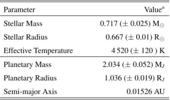
proper-ties of WASP-43b and its host star used in all the models are gathered in Table1.
Table 1. Properties of WASP-43 system.
Parameter Valuea Stellar Mass 0.717 (± 0.025) M Stellar Radius 0.667 (± 0.01) R Effective Temperature 4 520 (± 120 ) K Planetary Mass 2.034 (± 0.052) MJ Planetary Radius 1.036 (± 0.019) RJ Semi-major Axis 0.01526 AU
Reference.aGillon et al.(2012).
3. DESCRIPTION OF THE MODELS
3.1. Radiative Transfer Model
ATMOis a 1D/2D atmospheric model that solves the radia-tive/convective equilibrium with and without irradiation from an host star. It has been used for the study of brown dwarfs and directly imaged exoplanets (Tremblin et al. 2015,2016,
2017b;Leggett et al. 2016,2017), and also for the study of ir-radiated exoplanets (Drummond et al. 2016;Wakeford et al. 2017;Evans et al. 2017). The gas opacity is computed by using the correlated-k method (Lacis & Oinas 1991; Amund-sen et al. 2014,2017) including the following species in this study: H2-H2, H2-He, H2O, CO, CO2, CH4, NH3, K, Na,
Li, Rb, Cs from the high temperature ExoMol (Tennyson & Yurchenko 2012) and HITEMP (Rothman et al. 2010) line list databases. We use 32 frequency bins between 0.2 and 320 µm with 15 k-coefficients per bin. The chemistry is solved at equilibrium or out-of-equilibrium by a consistent coupling with the chemical kinetic network ofVenot et al.
(2012). 1D-ATMO has been recently benchmarked against
Exo-REMand petitCODE (Baudino et al. 2017).
In this study, we have used 2D-ATMO, an extension of 1D-ATMO (Tremblin et al. 2017a) that takes into account the circulation induced by the irradiation from the host star at the equator of the planet. We have taken a Kurucz spec-trum (Castelli & Kurucz 2004) for WASP-43 with a radius of 0.667 R , an effective temperature of 4500 K, and a gravity
of log(g) = 4.5. The magnitude of the zonal wind is imposed at the substellar point at 4 km/s and is computed accordingly to the momentum conservation law in the rest of the equa-torial plane. The vertical mass flux is assumed to be pro-portional to the meridional mass flux with a propro-portionality constant 1/α; the wind is therefore purely longitudinal and meridional if α → ∞ or purely longitudinal and vertical for α → 0. As inTremblin et al.(2017a), a relatively low value of
α drives the vertical advection of entropy/potential tempera-ture in the deep atmosphere that can produce a hot interior, which can explain the inflated radii of hot Jupiters. A high value of α will produce a "cold" deep interior as in the stan-dard 1D models. In this study, we have used two values of α, 10 and 104to explore these two limits. The simulation with
α=104should be more representative of WASP-43b since the planet is not highly inflated.
3.2. 3-D Circulation Models
SPARC/MITgcmcouples a state-of-the art non-grey,
ra-diative transfer code with the MITgcm (Showman et al.
2009). The MITgcm solves the primitive equations on a
cube-sphere grid (Adcroft et al. 2004). It is coupled to the non-grey radiative transfer scheme based on the plane-parallel radiative transfer code ofMarley & McKay(1999). The stellar irradiation incident on WASP-43b is computed with a Phoenix model (Hauschildt et al. 1999). The opacities we use are described inFreedman et al. (2008), including more recent updates (Freedman et al. 2014), and the molecu-lar abundances are calculated assuming local chemical equi-librium (Visscher et al. 2010). In the 3D simulation, the ra-diative transfer calculations are performed on 11 frequency bins ranging from 0.26 to 300 µm, with 8 k-coefficients per bin statistically representing the complex line-by-line opac-ities. For calculating the spectra the final SPARC/MITgcm thermal structure is post-processed with the same radiative transfer code but using a higher spectral resolution of 196 spectral bins (Fortney et al. 2006). We initialize the code with the analytical planet-averaged pressure-temperature profile ofParmentier et al.(2015a), run the simulation for 300 days and average all physical quantities over the last 100 days of simulation.
Our baseline model is a solar-composition, cloudless model. We also performed simulations including the pres-ence of radiatively active clouds and radiatively passive clouds following the method outlined in Parmentier et al.
(2016). Finally, models assuming a constant [CO]/[CH4]
ratio were also performed, following the method outlined in Steinrueck et al. (2018). These latter models simulate out-of-equilibrium transport-induced quenching of CO and CH4.
3.3. Chemical Kinetics Models
To address the variations of atmospheric chemical compo-sition with altitude and longitude, we used both 1D and 2D chemical kinetics models. We describe here these two codes.
3.3.1. 1D chemical kinetics model
The thermo-photochemical model developed by Venot
et al.(2012) is a full 1D time-dependent model. This model takes into account a detailed chemical kinetics and the out-of-equilibrium processes of photodissociation and vertical
mixing (eddy and molecular diffusion). The atmospheric composition is computed for a fixed thermal profile divided in discrete layers, solving the continuity equations for each species until steady-state is reached. No flux of species is imposed at the boundaries of the atmosphere. In this study, we used the C0-C2chemical kinetic network, which contains
∼ 2000 reactions describing the kinetics of 105 species made of H, C, O, and N, with up to two carbon atoms. This chem-ical scheme has been developed in close collaboration with specialists in combustion and validated experimentally on wide ranges of pressure and temperature as a whole (i.e. not only each reaction individually) leading to a high reliability. Since we consider both direction (forward and reverse) for each reaction, in absence of out-of-equilibrium processes, thermochemical equilibrium is achieved kinetically. To these ∼2000 reactions, 55 photodissociations have been added to model the interaction of incoming UV flux with molecules. These reactions are of course not reversed due to the dise-quilibrium irreversible nature of this process. A complete description of the model and the chemical scheme can be found inVenot et al.(2012). The kinetic model has been ap-plied to several exoplanetary atmospheres (Venot et al. 2012,
2013,2014,2016;Agúndez et al. 2014b;Tsiaras et al. 2016;
Rocchetto et al. 2016) and the deep atmosphere of Saturn (Mousis et al. 2014), Uranus (Cavalié et al. 2014,2017), and Neptune (Cavalié et al. 2017).
Using this 1D chemical kinetics model, we determined the chemical composition of the atmosphere of WASP-43b at different longitudes around the equator. The vertical temper-ature structure as a function of longitude is taken from the 2D radiative-transfer models (Section3.1) utilizing α=104since
the planet is not highly inflated. We extended these profiles to higher altitudes using extrapolation, and the resulting pro-files are shown in Fig.3. Each longitude has been computed until steady-state is reached, independently from each other, starting from the thermochemical equilibrium corresponding to the thermal structure. The stellar zenith angle varied with longitude. Given the characteristics of the host star, we es-timated the incident stellar spectrum using the same Kurucz (Castelli & Kurucz 2004) stellar model than in 2D-ATMO for wavelengths ≥ 2200 Å, an IUE spectrum of GL 15B scaled by a factor of 10 for the 1250-2200 Å region, and the solar maximum spectrum ofWoods & Rottman(2002) scaled by a factor of 1.36 (seeCzesla et al. 2013) for wavelengths less than 1250 Å. Vertical transport operates through eddy and molecular diffusion, with an assumed eddy diffusion coeffi-cient Kzzprofile that varies as Kzz(cm2s−1) = 107[P(bar)]−0.65
throughout the bulk of the planet’s infrared photosphere, in-dependent of longitude, except Kzz approaches a
constant-with-altitude value of 1010 cm2 s−1 at high altitudes and at
pressures greater than 300 bar (Figure 2). As a large un-certainty resides for this parameter, we chose to use an
ex-pression similar to the one adopted for HD 189733b based on GCM passive tracer transport (Agúndez et al. 2014a). This method gives values for the vertical mixing much lower (up to 1000 times) than the classical root-mean-square (rms) method (Agúndez et al. 2014a;Charnay et al. 2015). A cor-rect estimation of this parameter is crucial as it determines the quenching level and thus the molecular abundances of some fundamental species (e.g.Miguel & Kaltenegger 2014;
Venot et al. 2014;Tsai et al. 2017). Solar proportions of el-emental abundances are assumed (Lodders 2010) with a de-pletion of 20% in oxygen due to the sequestration in silicates and metals (Lodders 2004). No TiO/VO has been included.
3.3.2. 2D chemical kinetics model
Based on the procedure ofAgúndez et al.(2014a), for this study we developed a “pseudo-2D” chemical model to track how the atmospheric composition of WASP-43b would vary as a function of altitude and longitude, and hence orbital phase. We assume that longitudes are not isolated from each other (as in the 1D chemical model) rather connected through a strong zonal jet. Tidal interactions between host stars and gas giant planets are expected to circularize the planet or-bit and synchronize the rotation period of the planet (Lubow et al. 1997; Guillot & Showman 2002). The timescale for this to happen is much shorter than the stellar lifetime when the planet orbit is shorter than 10 days such as for WASP-43b (see Fig.1 ofParmentier et al. 2015b). With one hemi-sphere constantly facing the star, the unequal stellar forcing produces strong zonal winds that transport heat and chemi-cal constituents across the dayside and into the nightside of the planet, and back again (e.g., Showman et al. 2010; see also the GCM results in Section4.4). This zonal transport provides “diurnal” variation in temperatures and stellar irra-diation from the point of view of a parcel of gas being trans-ported by the winds. If chemical equilibrium were to prevail in WASP-43b’s atmosphere, the composition would be very different on the colder nightside in comparison to the hotter dayside. However, if the horizontal transport by the zonal winds is faster than the rate at which chemical constituents can be chemically converted to other constituents, then the composition can be “quenched” and remain more uniform with longitude (e.g., Cooper & Showman 2006; Agúndez et al. 2014a). Our pseudo-2D model tracks the time varia-tion in atmospheric composivaria-tion as a funcvaria-tion of altitude and longitude as an atmospheric column at low latitudes experi-ences this pseudo-rotation.
Our pseudo-2D thermo/photochemical kinetics model uses the Caltech/JPL KINETICS code (Allen et al. 1981) as its base, modified for exoplanets as described inMoses et al.
(2011,2013a,b,2016), along with the pseudo-2D procedure described in Agúndez et al. (2014a). The model contains 1870 reactions (i.e., 900 forward and reverse pairs)
involv-Pre ssu re (mb a r)
Eddy Diffusion Coefficient (cm2 s-1)
Kzz (cm 2 s-1) = 107 [P (bar)] -0.65 WASP-43b
Figure 2. The eddy diffusion coefficient profile adopted in our 1D and pseudo-2D thermo/photochemical models of WASP-43b. Our cloud microphysical model uses the same profile, except for pres-sures higher than 300 bar, where a lower limit value has been set at 107cm2s−1, to avoid numerical instabilities.
ing 130 different carbon-, oxygen-, nitrogen-, and hydrogen-bearing species whose rate coefficients have been reversed using the thermodynamic principle of reversibility (see Viss-cher & Moses 2011). Photolysis reactions are included and have not been reversed. The reaction list is taken from the GJ 436b model of Moses et al. (2013b), and includes H, C, O, N species. Molecules with up to six carbon atoms are included, but the possible chemical production and loss pathways in the model become less complete the heavier the molecule. Note that the chemical reactions list used in the pseudo-2D model slightly differs from that of the 1D chemical model. The departures between these two chem-ical schemes and their implications on the calculated abun-dances have already been addressed in several studies (Venot et al. 2012;Moses 2014;Wang et al. 2016): depending on the scheme used, the quench level and resulting quenched abundances of some species are somewhat different. For instance, for HD 209458b-like planets, the quenched mix-ing ratio of CH4 will be twice as large with Moses et al.
(2013b)’s scheme as with Venot et al.(2012)’s. However, the goal of our study here is to qualitatively compare the expected longitudinal variation obtained with the 1D and pseudo-2D chemical models in order to evaluate the effect of horizontal circulation on the global composition and trans-port/eclipse observations, and to determine a rough CO/CH4
ratio to be used in the 3D GCM. Comparing results between the 1D and pseudo-2D chemical models described here ade-quately addresses these goals. Other model inputs, including the boundary conditions and vertical diffusion coefficients adopted in the model, are identical to 1D chemical kinetics model described above.
Following Agúndez et al. (2014a), our pseudo-2D ap-proach is to solve the 1D continuity equations for a vertical column of gas at the equator as it rotates around the planet with a constant average low-latitude jet speed of 4.6 km s−1
(based on the GCM results described in Section4.4). As it has been discussed inAgúndez et al.(2012,2014a), assum-ing a uniform zonal wind is a good approximation for equa-torial region, dominated by a superrotating jet (Kataria et al. 2015). This approximation might be inadequate for latitudes towards the poles, when the circulation regime is more com-plex. Both the stellar zenith angle and atmospheric temper-atures vary with time as the gas column rotates through dif-ferent longitudes, both affecting the atmospheric chemistry. The vertical temperature structure as a function of longitude is fixed and is the same as that used in the 1D chemical kinet-ics model (Fig.3). The eddy diffusion profile (Kzzcoefficient
profile) is also similar to that of the 1D chemical kinetics model (Fig.2). The planet is divided into different longitude regions, and the system of differential equations making up the continuity equations is integrated over the amount of time it would take a parcel of gas at the equator to be transported from one discretized longitude to the next discretized longi-tude. At that point, the mixing ratios as a function of pressure at the end of the first longitude calculation are fed in as ini-tial conditions to the next longitude calculation, with its new thermal structure and incident UV flux that depends on the new zenith angle. The temporal evolution of this equatorial column of gas is followed for 20 full planetary “rotations” to provide sufficient time for the species produced photochem-ically at high altitudes to be transported down through the atmosphere to deeper regions where thermochemical equi-librium dominates. At that point, the “daily” longitude vari-ations were consistent from one pseudo-rotation to the next.
Agúndez et al.(2012) discuss the various advantages of be-ginning the pseudo-2D calculations at the hottest dayside conditions. Based on their discussion, we use the results of a 1D thermo/photochemical kinetics model for conditions at the substellar point (longitude 0˚) that has been run long enough to reach steady state as our initial conditions for the pseudo-2D model.
3.4. Cloud Microphysics Model
We use the Community Aerosol and Radiation Model for Atmospheres (CARMA;Turco et al. 1979;Toon et al. 1988;
Jacobson & Turco 1994; Ackerman et al. 1995) to inves-tigate the vertical and longitudinal distribution of clouds in the atmosphere of WASP-43b. While we do not include the resulting distributions in our GCM simulations, we will be able to extract insights into the effect of longitudinal temper-ature variations on cloud distributions. CARMA is a 1D cloud microphysics model that generates binned size distributions of aerosol particles as a function of altitude (pressure) in an
Longitude: Pre ssu re (mb a r) Temperature (K) CO CH4 N a 2S (co nd) Mg Si O 3 (co nd ) Mg 2Si O 4 (co nd )
Figure 3. Equatorial temperature profiles at different longitudes (colored solid lines, as labeled) adopted in our 1D and pseudo-2D thermo/photochemical models. Temperatures were derived from the 2D radiative-transfer model described inTremblin et al.(2017a), for an assumed alpha value of 10,000 (uninflated radius, cold interior). The dashed black curve shows where CO and CH4would have equal
abundance in chemical equilibrium for solar composition: CO dom-inates at lower pressures and higher temperatures, while CH4
dom-inates at lower temperatures and higher pressures. The black and gray dot-dashed lines show the equilibrium condensation curves for MgSiO3, Mg2SiO4, and Na2S for a solar composition atmosphere.
atmospheric column by explicitly computing and balancing the rates of cloud particle nucleation, growth by condensa-tion and coagulacondensa-tion, loss by evaporacondensa-tion, and transport by sedimentation, advection, and diffusion. This sets CARMA apart from simpler cloud condensation models (e.g.Fegley & Lodders 1994;Ackerman & Marley 2001), which assume cloud formation as soon as the condensate vapor saturates. The equations CARMA solves to evaluate the rates of these processes are presented in the Appendix ofGao et al.(2018). CARMAhas been applied to aerosol processes across the solar system (Colaprete et al. 1999;Barth & Toon 2003;Bardeen et al. 2008;Gao et al. 2014;Gao et al. 2017), and has recently been used to simulate Al2O3, TiO2, MgSiO3(enstatite), KCl,
and ZnS clouds on exoplanets and brown dwarfs (Gao et al. 2018;Powell et al. 2018;Gao & Benneke 2018).
For this work, we include additional condensates that have been hypothesized to dominate the condensate mass in exo-planet atmospheres, including Mg2SiO4(forsterite), Fe, Cr,
MnS, and Na2S (Lodders 1999;Visscher et al. 2006;Helling
et al. 2008;Visscher et al. 2010). Additional condensates are possible, as shown in grain chemistry models (e.g.Helling & Woitke 2006), but we do not treat them here, as it would be computationally prohibitive. In addition, to reduce the number of different condensates we assume that forsterite is the primary silicate condensate rather than modeling both forsterite and enstatite clouds. This is based on the argument that a rising parcel of vapor would see forsterite condense
first due to it having higher condensation temperatures than enstatite; this depletes Mg and SiO, such that the enstatite cloud that forms above the forsterite cloud should have sig-nificantly lower mass. We discuss the implications of this assumption in the Sect. 4.3. As with the treatment of en-statite inPowell et al.(2018), we assume forsterite and Fe clouds form by heterogeneously nucleating on TiO2 seeds,
as direct nucleation of these two species from vapor is slow (Helling & Woitke 2006;Gao et al. 2018). All other conden-sates are assumed to nucleate homogeneously.The saturation vapor pressures of Cr, MnS, and Na2S are taken fromMorley
et al.(2012). The surface energy of Cr is calculated from the Eötvös rule, while for MnS and Na2S we assume the same
surface energy as that of KCl. The size distribution for each condensate species is calculated separately, and so a distinct size distribution exists for each species.
As in the 1D and pseudo-2D chemical kinetics models, we use fixed pressure-temperature profiles described in Section
3.1for our background atmosphere. All planetary parame-ters used are the same as those of the other models presented here to ensure consistency. In the cloud microphysics model, we use a very similar Kzzprofile as the one used in the
chem-ical kinetics models (Figure2), except we set a minimum Kzz
of 107 cm2 s−1. This change only affects pressures >1 bar,
where the chemical kinetics model Kzzis <107cm2s−1. We
also reduce the high Kzz at pressures >300 bar to our
min-imum value. This was necessary to reduce model run time and numerical instabilities. An atmospheric column is sim-ulated at each longitude independently of each other, under the assumption that microphysical timescales are short com-pared to horizontal transport timescales, though this may not be the case for all pressure levels and particle sizes ( Pow-ell et al. 2018). For each column, we investigate distinct clouds composed of Al2O3, TiO2, Mg2SiO4, Fe, Cr, MnS,
Na2S, ZnS, and KCl, though which clouds actually form
de-pends on which species is supersaturated and their nucleation rates. We assume solar abundances for the limiting elements of these clouds, which are, in the same order, Al, TiO2, Mg,
Fe, Cr, Mn, Na, Zn, and KCl.
Importantly, the vertical, longitudinal, and particle size dis-tributions computed by this model are not used to generate synthetic observations, as will be presented later in this work. This is due to the uncertainties in the material properties of some of the condensates (e.g. surface energies of MnS and Na2S) and the way exoplanet clouds form, whether through
homogeneous nucleation, heterogeneous nucleation on some foreign condensation nuclei, or grain chemistry (Helling & Woitke 2006). Instead, results from CARMA will be help-ful for informing general GCM and retrieval studies due to its ability to compute the relative abundances of different cloud species in the atmosphere of WASP-43b, thus indicat-ing the species that affect the observations the most.
Simpli-fied cloud models can then be used to explore the parameter space around these results.
3.5. JWST Observation Model
WASP-43b is the primary target for the “MIRI Phase Curve” observation that will be carried out as part of the Transiting Exoplanet JWST Early Release Science Program. The goal is to observe a full orbit of WASP-43b including two eclipses and one transit in the wavelength range 5–12 µm at a resolution R ∼ 100 with MIRI LRS (Low Resolution Spec-troscopy) in slitless mode (Kendrew et al. 2015). In that pro-gram, the planetary emission spectra as a function of longi-tude will be measured and relevant atmospheric properties retrieved. We simulate the expected outcomes of this ob-servation using the PandExo2 software program (Batalha
et al. 2017). PandExo is a noise simulator specifically designed for transiting exoplanet observations with JWST and HST, and includes all observatory-supported time-series spectroscopy modes.
The input parameters for the star and planet are those in-dicated in Table1. The stellar spectrum is obtained from the NextGen(Hauschildt et al. 1999) grid interpolated at the Teffand log(g) of WASP-43 and is the same as used in the 3D
SPARC/MITgcm. We consider a range of planetary emis-sion spectra derived from the 3D SPARC/MITgcm model described in Section3.2, with or without clouds, assuming thermochemical equilibrium or a quenched [CH4]/[CO]
ra-tio. These simulations are performed with similar inputs as those used for the JWST ERS Program proposal (PIs: N. Batalha, J. Bean, K. Stevenson; Bean et al. 2018): the ra-diative transfer models, the star and planet parameters and input spectra, and the observation parameters are the same (here we simulate a broader range of planetary spectra).
The planetary spectra are calculated from the emission in-tegrated over the visible hemisphere. For this work, we sim-ulate spectra with a spacing of 20˚ in longitude and use them as inputs for PandExo. We consider that we observe each longitude during one eighteenth of the orbital period (1.08 hours) and we use a baseline of twice the eclipse duration because we will observe two eclipses (2.32 hours). In prac-tice, the longitude 0˚ will be in-eclipse so we may have to split the orbit slightly differently, but for these simulations we treat this longitude as the other ones. The resolution and instrumental parameters are those of MIRI LRS. The wave-length range goes up to ∼ 14 µm but we consider only the 5–12 µm range because the efficiency of LRS decreases sig-nificantly beyond 12 µm. We use a saturation level of 80% of the full well. The details of the noise modelling can be found inBatalha et al.(2017).
2https://exoctk.stsci.edu/pandexo/
3.6. Retrieval models
To retrieve the atmospheric properties of WASP-43b, we use two models: TAUREX3(Waldmann et al. 2015b,a; Roc-chetto et al. 2016) and the Python Radiative Transfer in a Bayesian framework (PYRAT BAY4, Cubillos et al. 2019, in prep., Blecic et al. 2019a,b, in prep.). Both, TAUREX and PYRAT BAYare open-source retrieval frameworks that compute radiative-transfer spectra and fit planetary spheric models to a given set of observations. The atmo-spheric models consist of parameterized 1D profiles of the temperature and species abundances as a function of pres-sure, with atomic, molecular, collision-induced, Rayleigh, and cloud opacities. We decide to use two codes that don’t use the same retrieval methods in order to compare the results obtained and raise the eventual biases that could emerge. We present hereafter the two codes.
3.6.1. TAUREX
The TAUREX model can retrieve equilibrium chemistry using the ACE code (Agúndez et al. 2012) as well as per-form so-called “free” retrievals where trace gas volume mix-ing ratios are left to vary as free parameters. For this study, all the retrieval models used the “free chemistry” method. The statistical sampling of the log-likelihood is performed using nested sampling (Skilling 2006; Feroz et al. 2009). TAUREXis designed to operate with either absorption cross-sections or correlated-k coefficients. Both cross-cross-sections and k-tables were computed from very high-resolution (R > 106).
Cross-sections are calculated from ExoMol (Tennyson et al. 2016), HITEMP (Rothman et al. 2010) and HITRAN ( Gor-don et al. 2017) line lists using ExoCross (Yurchenko et al. 2018). In particular, for this study we used the following ele-ments: H2O (Barber et al. 2006), CO (Rothman et al. 2010),
CO2 (Rothman et al. 2010), and CH4 (Yurchenko &
Ten-nyson 2014), H2 and He. Rayleigh scattering is computed
for H2, CO2, CO and CH4 (Bates 1984; Naus & Ubachs
2000;Bideau-Mehu et al. 1973;Sneep & Ubachs 2005) and collision induced absorption coefficients (H2- H2, H2- He)
are taken fromRichard et al.(2012). Temperature and pres-sure dependent line-broadening was included, taking into ac-count J-dependence where available (Pine 1992). The ab-sorption cross-sections were then binned to a constant reso-lution of R = 15000 and the emission forward models were calculated at this resolution before binning to the resolution of the data during retrievals. TAUREXcan consider grey and Mie scattering clouds (Toon & Ackerman 1981), as well as the Mie opacity retrieval proposed byLee et al.(2013). The temperature-pressure profiles used in this study are
parame-3https://github.com/ucl-exoplanets 4http://pcubillos.github.io/pyratbay
terised by analytical 2-stream approximations (Parmentier & Guillot 2014;Parmentier et al. 2015a).
3.6.2. PYRATBAY
PYRATBAYexplores the parameter space via a Differential-evolution MCMC sampler (Cubillos et al. 2017), allowing both “free” and “self-consistent” (equilibrium chemistry) retrieval.
The “free” retrieval fits for the thermal structure using the parameterized temperature profiles of Parmentier & Guil-lot(2014) used byLine et al.(2013), constant-with-altitude abundances for H2O, CH4, and CO; and either one of the
cloud parametrization models (detailed later in this Section). In this study, we neglect CO2because it does not contribute
significantly in the spectrum of WASP-43b modelled by our Global Circulation Model on which the retrieval is per-formed, contrary to models of (Mendonça et al. 2018b) where CO2 is proposed as a potential absorber on the nightside of
the planet.
For “self-consistent” retrievals, we fit for the temperature and cloud parameters while assuming chemical equilibrium and solar elemental abundances. The chemical equilibrium is calculated with a newly developed open-source analytic thermochemical equilibrium scheme called RATE, Reliable Analytic Thermochemical-equilibrium Abundances ( Cubil-los et al. 2019), a similar, but more widely applicable ap-proach thanHeng & Tsai(2016). For this study, we include only H2O, CH4, CO, CO2, and C2H2 abundances and fix
the elemental abundances to the solar ones ofAsplund et al.
(2009)5.
For the opacities PYRATBAYconsiders line-by-line opaci-ties sampled to a constant wavenumber sampling of 0.3 cm−1
for the four main spectroscopically active species expected at the probed wavelengths: H2O (Rothman et al. 2010), CH4
(Yurchenko & Tennyson 2014), CO (Li et al. 2015), and CO2 (Rothman et al. 2010). (The same species considered
in TAUREXbut with different references for CO and H2O).
Since these databases consist of billions of line transitions, we first apply our repacking algorithm (Cubillos 2017) to ex-tract only the strong line transitions that dominate the opac-ity spectrum between 300 and 3000 K. Our final line list contains 5.5 million transitions. Additionally, PYRAT BAY considers Rayleigh opacities from H2(Lecavelier Des Etangs
et al. 2008), collision-induced absorption from H2–H2 (
Bo-rysow et al. 2001;Borysow 2002) and H2–He (Borysow et al.
1988, 1989; Borysow & Frommhold 1989). PYRAT BAY implements several cloud parameterization models: a
sim-5In general RATE is able to calculate the abundances of twelve
atmo-spheric species (H2O, CO, CO2, CH4, C2H2, C2H4, H2, H, He, HCN, NH3,
and N2) for arbitrary values of temperatures (200 to ∼2000 K), pressures
(10−8to 103bar), and C, N, O abundances (10−3to ∼102× solar elemental
abundances).
ple opaque gray cloud deck at a given pressure, a thermal-stability cloud approach described in Blecic et al. (2019a, in prep.), and a kinetic, microphysical cloud parameterization model (Blecic et al. 2019b, in prep.). In all complex cloud models the cloud opacity is calculated using Mie-scattering theory (Toon & Ackerman 1981).
For cloud-free retrieval, PYRAT BAYuses a top pressure of a gray cloud deck in his cloud-free model. For cloudy retrievals in this study, we use our Thermal Stability Cloud (TSC) model (Blecic et al. 2019a, in prep.) to retrieve the longitudinal cloud structure (see alsoKilpatrick et al. 2018). The model is based on the methodology described in Ben-neke(2015) andAckerman & Marley(2001) with additional flexibility in the location of the cloud base depending on the local metallicity of the gaseous condensate species just below the cloud deck.
The PYRAT BAY code explores the posterior parameter space with the Snooker differential-evolution MCMC (ter Braak & Vrugt 2008), obtaining between 1 and 4 million samples, with 21 parallel chains (discarding the initial 10 000 iterations), while ensuring that theGelman & Rubin(1992) statistics remain at ∼1.01 or lower for each free parameter.
4. RESULTS OF ATMOSPHERIC MODELS
4.1. Atmospheric structure
The pressure/temperature structure of the atmosphere can be constrained with 2D and 3D models. A comparison is
given in Fig. 4 between the 3D SPARC/MITgcm model
and the 2D-ATMO model with the two cases of interior: the hottest one (α=10) and the coldest one (α=104). For the two
α values, the upper atmosphere is similar. In this part (pres-sures less than 1 bar), the agreement between the 2D and the 3D models is quite remarkable since there is no tuning of the 2D model on the 3D model apart from the choice of hori-zontal wind speed. Since the chemistry and radiative transfer models are independent between the two codes, this agree-ment is also a sign that convergence between different GCMs and 2D steady-state circulation models can be reached for the pressure/temperature structure at and above the photosphere. As explained in Sect. 3.1, for pressures greater than 1 bar, the different α values lead to different temperatures in the deep atmosphere. Because the GCM is not fully converged at pressures larger than 10 bars, it likely produces spurious vari-ations of the deep pressure-temperature profile. The shape of the deep flow structure and its influence in the upper atmo-spheric dynamics is still an active subject of research (Mayne et al. 2014,2019;Carone et al. 2019) and out of the scope of this paper. Given that both the GCM and the 2D model pro-duce very similar thermal structure in the observable atmo-sphere we decided to use the outputs of the 2D model as in-puts for the chemical and cloud formation models. We opted for the cold interior model (α=104) based on the ground that
������� ������� ������� ������ ����� ���� �� ��� ���� ���� ����� ����� ����� ����� ��������������� ������������������������������ �� ��� ���� ����� ���� � ��������������� ������� ������� ������� ������� ������ ����� ���� �� ��� ���� ���� ����� ����� ����� ����� ��������������� ������������������������������ �� ��� ���� ����� ���� � ��������������� �������
Figure 4. Comparison of the equatorial temperature structure predicted by the 3D SPARC/MITgcm model with the 2D-ATMO model assuming α = 10 (top) and α = 104(bottom).
the planet does not appear to be highly inflated. However, a more thorough investigation of the deep thermal structure on the observable cloud properties (e.g.Powell et al. 2018) will be needed in the future to interpret the observations.
4.2. Chemical composition
We study the chemical composition of WASP-43b at dif-ferent longitudes with our 1D and pseudo-2D models. The results are presented in Fig.5, together with the abundances at thermochemical equilibrium, corresponding to the same longitude-variable thermal structure. In the 1D model, all the longitudes have been computed independently, assuming thermochemical composition as initial composition at each longitude. The different vertical columns don’t interact with each other. In the pseudo-2D model, the longitudes are not independent interacting through horizontal circulation. As we explained in Sect.3.3, the steady state composition of the substellar point is given as initial condition to the adjacent longitude. There, the evolution of chemical composition is
calculated over the amount of time necessary for a parcel of gas to reach the next longitude, and so on.
In all models, as the temperature is identical at each lon-gitude for pressures greater than ∼103 mbar, we find that species have also the same abundances, corresponding to the thermochemical equilibrium values. The composition varies with longitude above this region, more or less depending on species. For pressures lower than ∼103mbar, many of the
at-mospheric constituents would vary significantly with longi-tude if the atmosphere remained in thermochemical equilib-rium throughout. Particularly noteworthy is the fact that CH4
would be the dominant carbon-bearing constituent at high al-titudes on the colder nightside in thermochemical equilib-rium, while CH4 would virtually disappear from the
day-side and CO would become the dominant carbon-bearing constituent at all altitudes. The 1D kinetic model predicts that vertical quenching will reduce this variation, but there are still several orders of magnitude differences between the abundances of the dayside and that of the nightside. In con-trast, the pseudo-2D model predicts much less variation with longitude, particularly in the 0.1–1000 mbar region that is probed at infrared wavelengths. The CO that forms on the hot dayside cannot be chemically converted to CH4quickly
enough on the nightside, before the atmospheric parcels are carried by the zonal winds back to the dayside. These results confirm the findings byCooper & Showman(2006), Agún-dez et al.(2014a),Mendonça et al.(2018b),Drummond et al.
(2018a) andDrummond et al.(2018b) that both vertical and horizontal chemical quenching are important in hot Jupiter atmospheres.
Another species whose abundance predicted by our kinetic model is very different from what is expected by thermo-chemical equilibrium is HCN. At thermothermo-chemical equilib-rium, this species has the same abundance profile at each longitude, and its abundance decreases with increasing al-titude. The 1D kinetic model predicts that this species will be quenched at around 102 mbar, leading to a higher
abun-dance than what is predicted by thermochemical equilibrium on the nightside, and even higher abundance on the dayside thanks to a photochemical production. Note that the quench-ing pressure we determine with our model is of course highly dependent on the Kzzprofile we assume. At 102mbar, KZZis
about 4.5×107 cm2 s−1. As we said in Sect. 3.3, this
pa-rameter is rather uncertain and could vary by several orders of magnitude (typically 106–1012 cm2 s−1 among
Parmen-tier et al. 2013;Agúndez et al. 2014a). Consequently, with these extreme values, the pressure level quenching of HCN could vary between 10 and 105 mbar. In contrast to what has been found with the 1D kinetic model, our pseudo-2D model indicates that the abundance of HCN on the night-side will remain very high and close to that of the daynight-side thanks to the horizontal circulation, in agreement with
Agún-dez et al. (2014a). A such high abundance might be de-tectable thanks to high-resolution spectroscopic observations in the near-infrared coupled to a robust detrending method (Hawker et al. 2018; Cabot et al. 2019). On JWST/MIRI observations, HCN could eventually appear in the 7–8 µm band, albeit spectra will probably be dominated by water ab-sorption in this region given the important abundance of H2O
in the atmosphere of WASP-43b (Rocchetto et al. 2016). Similarly toAgúndez et al. (2014a), we find that in ad-dition to vertical quenching due to eddy diffusion, the hori-zontal circulation leads to horihori-zontal quenching of chemical species. Globally, the atmosphere of WASP-43b has a chem-ical composition homogenized with longitude to that of the dayside. This is particularly true for pressures larger than 1 mbar, while variations of abundances between the day and nightside still remain at lower pressures.
In summary, the pseudo-2D model suggests that CH4
would be a relatively minor constituent on WASP-43b at all longitudes, that photochemically produced HCN will be more abundant than CH4 in the infrared photosphere of
WASP-43b at all longitudes, and that the key spectrally ac-tive species H2O and CO will not vary much with longitude
on WASP-43b. Benzene (C6H6) is a proxy for
photochem-ical hazes in the pseudo-2D model, and the strong increase in the benzene abundance at nighttime longitudes suggests that refractory hydrocarbon hazes could potentially be pro-duced at night from radicals propro-duced during the daylight hours (e.g.Miller-Ricci Kempton et al. 2012;Morley et al. 2013,2015). Note that a recent experimental study demon-strates that refractory organic aerosols can be formed in hot exoplanet atmospheres with a C/O ratio higher than solar (Fleury et al. 2019).
Based on these chemical models and because the variation of CH4with longitude could be observed with MIRI, we ran
GCMs assuming chemical equilibrium and assuming a fixed [CH4]/[CO] ratio of 0.001, which is representative of the 2D
chemical model in the 0.1-1000 mbar region.
4.3. Cloud coverage
We use the CARMA model to determine the physical and chemical properties of the clouds along different ver-tical columns at the equator of the planet. Assuming Mie-scattering particles, we calculate the cloud optical depth pro-file for each longitude from 0.35 to 30 µm. Fig. 6 (top) shows the pressure levels at which the total cloud column optical depth (taking into account all cloud species) equals 1, and reveals large differences between the day and night sides. Specifically, the day side temperature profile is such that most of the forsterite (Mg2SiO4) is cold trapped
be-low 100 bars, and although the forsterite condensation curve crosses the temperature profile again at lower pressures, the
10-1210-1110-10 10-9 10-8 10-7 10-6 10-5 10-4 10-3 10-2 Mole fraction 10-8 10-7 10-6 10-5 10-4 10-3 10-2 10-1 100 101 102 103 104 105 106 Pr essu re
(m
ba
r)
CO
2HCN
NH
3CH4
N
2CO
H
2O
night day night day(a)
WASP-43b equilibrium as fct of longitude
10-1210-1110-10 10-9 10-8 10-7 10-6 10-5 10-4 10-3 10-2 Mole fraction 10-8 10-7 10-6 10-5 10-4 10-3 10-2 10-1 100 101 102 103 104 105 106 Pr essu re
(m
ba
r)
CO
2HCN
NH
3CH4
N
2CO
H
2O
nig ht day night day nig ht day(b)
WASP-43b 1D chem as fct of longitude
10-1210-1110-10 10-9 10-8 10-7 10-6 10-5 10-4 10-3 10-2 Mole fraction 10-8 10-7 10-6 10-5 10-4 10-3 10-2 10-1 100 101 102 103 104 105 106 Pr essu re
(m
ba
r)
CO
2HCN
NH
3CH4
N
2CO
H
2O
nig ht day night day(c)
WASP-43b pseudo-2D chem as fct of longitude
Figure 5. Mixing ratio profiles for important atmospheric con-stituents on WASP-43b (as labeled) at 10 different longitudes across the planet (every 36 degrees) from (a) a model that assumes thermo-chemical equilibrium, (b) our 1D thermo/photothermo-chemical model that tracks chemical kinetics and vertical transport, or (c) our pseudo-2D model that tracks in addition horizontal transport.
100 101 Wavelength
(
μm)
10
210
310
410
5Pr
es
su
re
(m
ba
r)
0 deg 36 deg 72 deg 108 deg 144 deg 180 deg 216 deg 252 deg 288 deg 324 deg10
010
110
2Effective Particle Radius (
μm)
10
210
310
410
5Pr
es
su
re
(m
ba
r)
Figure 6. Pressure levels where the total cloud column optical depth equals 1 (top) and the effective particle radius profiles (bottom) pre-dicted by CARMA for the labeled longitudes. The effective particle radius is calculated by averaging the size distributions of the indi-vidual cloud species; the actual mean particle radii of each species range from 0.01 to 100 µm and are functions of altitude (pressure).
abundance of Mg there is sufficiently low so as to prevent optically thick clouds from forming (Fig.7).
On the night side, sufficiently low temperatures allow for the condensation of optically thick MnS and Na2S clouds,
such that the optical depth = 1 pressure level is above 0.1 bar blueward of 7 µm. As the typical particle sizes of these clouds are 1 to a few µm (Fig. 6, bottom), they become optically thin at longer wavelengths, allowing for forsterite clouds to become visible, as shown by the 10 µm silicate feature. Note that this forsterite cloud is not the cold-trapped cloud at 100 bars. Instead, because the forsterite conden-sation curve crosses the temperature profile a second time at higher pressures here than on the day side, there is suffi-cient Mg to produce an optically thick “upper” cloud even after accounting for cold trapping. The shape of the effec-tive particle radius profiles shown in Fig.6(bottom) also re-veals this transition in cloud composition with longitude, as particle size tends to increase towards the cloud base due to available condensate vapor supply and size sorting by loft-ing and sedimentation. For example, while day side pro-files are largely smooth, corresponding to the dominance of
the forsterite cloud, the night side profiles feature a MnS cloud deck above 1 bar sitting atop the forsterite cloud be-low (Fig.7).
Our results suggest that whether forsterite or enstatite is considered the primary silicate condensate could strongly im-pact the dayside cloud opacity. As enstatite condenses at lower temperatures (Fig.3), it would not form a deep cloud at pressures > 100 bars on the day side, like forsterite. This lack of cold trapping may result in an optically thick cloud at lower pressures. This is in contrast to the nightside, where forsterite only dominates the cloud opacity at long wave-lengths. We therefore expect that, since the cloud base of forsterite is only ∼50% higher in pressure than enstatite, forsterite will have similar effect on the night side spectra as enstatite. Whether the forsterite or enstatite clouds are cold trapped in the deep atmospheric layers depends on both mi-crophysical behavior of the cloud (studied here), the strength of the vertical mixing and the temperature in the deep atmo-sphere (Powell et al. 2018).Thorngren et al.(2019) recently predicted a connection between planet equilibrium temper-ature and their intrinsic flux, suggesting that cold traps on certain hot Jupiters may not exist due to high temperatures in the deep atmosphere. By determining the cloud chemi-cal composition in the nightside of WASP-43b through our JWST/MIRI phase curve observation will provide insights into the presence of a deep cold trap and thus test the pre-dictions fromThorngren et al.(2019).
Our work decouples cloud microphysics from the radiation field and dynamics of the rest of the atmosphere, and thus we cannot treat cloud radiative feedback or cloud advection. Fully coupled 3D models that include cloud microphysics in the form of grain chemistry have been applied to other in-dividual exoplanets in the past, including HD 189733b and HD 209458b, which have similar temperatures to WASP-43b (Helling et al. 2016;Lee et al. 2016; Lines et al. 2018a,b). These works show that the mean particle radii vary between 1-100 µm between 0.1 and 100 bars, and that the composition of mixed cloud particles is dominated by enstatite, forsterite, iron, SiO, and SiO2, with forsterite being more abundant than
enstatite at most longitudes. This is similar to our results, though we do not consider SiO and SiO2in our model, while
they do not consider sulfide clouds in theirs. Advection tends to smooth out cloud composition differences, which we do not capture in our work. One other major difference between the grain chemistry models and our model is the high abun-dance of small particles at low pressures in grain chemistry models stemming from high nucleation rates at low pres-sures. In contrast, nucleation rates are the highest at the cloud base in our model (Gao et al. 2018) owing to the high atmo-spheric density there, and so we lack a low pressure, small particle population.
0.0 0.2 0.4 0.6 0.8 1.0 Opacity Fraction
0 deg 36 deg 72 deg 108 deg 144 deg
100 101 Wavelength ( m) 0.0 0.2 0.4 0.6 0.8 1.0 Opacity Fraction 180 deg 100 101 Wavelength ( m) 216 deg 100 101 Wavelength ( m) 252 deg 100 101 Wavelength ( m) 288 deg 100 101 Wavelength ( m) 324 deg
Al
2O
3TiO
2Fe
Mg
2SiO
4Cr
MnS
Na
2S
ZnS
KCl
Figure 7. Contributions to the optical depth from each simulated cloud species at the pressure level where the total cloud column optical depth equals 1, as computed by CARMA for the labeled longitudes. Each cloud species is constituted in homogeneous particles except for forsterite and Fe, which have TiO2cores.
To summarize, our results show that, if silicates primarily form forsterite clouds, then the day side of WASP-43b should be cloudless down to 100 bars, while the night side cloud opacity should be dominated by MnS and Na2S clouds
short-ward of 7 µm, and forsterite clouds at longer wavelengths. Cloud particle sizes on the night side at the pressure levels where clouds become opaque are on the order of 1 to a few µm. On the other hand, if silicates primarily form enstatite clouds, then the dayside should be cloudier at pressures <100 bars, while the nightside cloud opacity would remain domi-nated by the sulfide clouds.
4.4. 3-D thermal structure
We use our 3D model to calculate the thermal structure of WASP-43b assuming different chemical composition (ther-mochemical equilibrium and disequilibrium) and cloudy
conditions (clear, MnS, and MgSiO3). The temperature
structure and CH4 abundances for the cloudless chemical
equilibrium and disequilibrium simulations are shown in Fig. 8. From these models, we calculate the corresponding emission spectra at dayside and nightside.
The thermal structure of our cloudless, chemical equi-librium SPARC/MITgcm simulations are very similar to the one presented in Kataria et al.(2015) where the reader can find a thorough description of the atmospheric flows. While Kataria et al. (2015) focused on the effect of TiO, metallicity and drag, we hereafter discuss the role of disequi-librium chemistry and clouds in shaping the nightside spec-trum of the planet.
In the case of quenched carbon chemistry ([CH4]/[CO] =
0.001), the dayside is slightly cooler and the nightside is slightly warmer at a given pressure level than for our chemi-cal equilibrium case. However, the differences in the spectra seen in Fig.9are mainly due to change in the opacities rather than changes in the thermal structure. On the dayside, where
45 0 45
latitude [deg]
Equilibrium chemistry Quenched case
90 0 90 longitude [deg] 45 0 45 latitude [deg] -6 -8 -6 -4 -4 -4 -4 90 0 90 longitude [deg] 750 1000 1250 1500 T [K] 9.0 7.5 6.0 4.5 log10 (XCH 4 )
Figure 8. Temperature (top) and methane abundance (bottom) at the 30 mbar level from our 3D simulations. The substellar point is at 0◦ longitude. The simulation assuming thermochemical equilibrium is shown to the left and the simulation assuming quenched CH4, CO
and H2O abundances is shown to the right.
the [CH4]/[CO] ratio is small at chemical equilibrium, our
quenched and chemical equilibrium simulations are indistin-guishable. On the nightside, the quenching removes the CH4
absorption bands between 3 and 4 µm and the ones between 7 and 9 µm are weakened in the quenched scenario, leading to a signature detectable by JWST/MIRI. Note that our GCM simulations approximate the [CH4]/[CO] ratio to be constant
throughout the atmosphere (horizontally and vertically) for computational reasons, while the pseudo-2D simulations in Section4.2as well as 3D simulations of WASP-43b with a simplified chemistry scheme (Mendonça et al. 2018b) find that the methane abundance is homogenized horizontally but decreases with increasing altitude. However,Steinrueck et al.
(2018) found that the effect of disequilibrium chemistry on the thermal structure and phase curve is qualitatively similar for different constant [CH4]/[CO] ratios as long as CO is the
dominant carbon-bearing species. Therefore, it is likely that the effect of a horizontally homogenized [CH4]/[CO] ratio
�� ����� ����� ����� ����� �� ��� ����������� ������ ��������� �������� ��������� � � ������������ ��������������� ���������� ������������� � � ������� ��������� ���� ���������� ��� ��� ��� ���� ����
Figure 9. Dayside (plain) and nightside (dashed) spectrum of WASP-43b predicted by the SPARC/MITgcm for cloudless, cloudy (with 1 µm particles) or non-equilibrium assumptions. Current HST and Spitzer (Stevenson et al. 2017;Mendonça et al. 2018a) obser-vations are shown as dots, planned JWST/MIRI obserobser-vations are shown as triangles. ��� ���� ���� ���� ���� �� ��� ����������� ������ ��������� �������� ��������� ������������ ��� ������ ����� ��� ���� ���� ���������� ��� ��� ��� ���� ����
Figure 10. Dayside (top curve) and nightside (bottom curves) spectrum of WASP-43b predicted by the SPARC/MITgcm for our cloudless models and models with passive MnS (blue) and MgSiO3
(red) clouds of different particle sizes. Current HST and Spitzer ob-servations are shown as dots, planned JWST/MIRI obob-servations are shown as triangles.
quenched simulation thus still provides a valuable estimate of the effects of disequilibrium chemistry.
The cloudless simulations were also post-processed with cloud opacities. The post-processing allows for a quick esti-mate of the strength of potential signature of cloud properties in the emission spectrum without the need to run additional, time-consuming, global circulation models. In Sect.4.3, we found that the nightside of WASP-43b could be dominated by MnS, Na2S, MgSiO3, and/or Mg2SiO4. Following
0 2000 4000 6000 8000 1 10 Fp/Fs (ppm) λ (µm) Stevenson Mendonca JWST/MIRI Clear, solar Passive clouds Active clouds Dayside Nightside Data GCM Models 0 300 600 1.3 1.6
Figure 11. Dayside (top curve) and nightside (bottom curves) spectrum of WASP-43b predicted by the SPARC/MITgcm for our cloudless models, models with passive MnS, 1µm clouds (blue) and models with radiatively active MnS, 1µm clouds (red). Current HST and Spitzer observations are shown as dots, planned JWST/MIRI observations are shown as triangles.
mentier et al.(2016), we explore two possible cloud compo-sitions: MnS and MgSiO3. Forsterite and enstatite having
opacities and condensation curves very similar, we chose to include just one of these silicate species. As we found with our microphysical cloud model (Sect. 4.3), the atmosphere
of WASP-43b is cool enough for MgSiO3 clouds to cover
the whole planet affecting both the dayside and the night-side of the planet. Conversely, MnS clouds can only form on the cooler nightside and thus only affect the nightside’s spectrum. Both MnS and MgSiO3 clouds are able to
suffi-ciently dim the nightside emission spectrum blueward of 5 µm in order to match the HST and the Spitzer observations. As shown in Fig.9, in all our models the nightside flux re-mains observable with JWST/MIRI, even when the thermal emission is extremely small shortward of 5 µm. MnS and MgSiO3cloud composition could be distinguished spectrally
by our JWST/MIRI phase curve observation through the ob-servation of the 10 µm absorption band seen in the red mod-els of Fig.9(see alsoWakeford & Sing 2015).
The effect of the cloud particle size is explored in Fig.10. Assuming that the formation of MnS clouds is limited by the available amount of manganese in a solar-composition atmo-sphere, the MnS clouds could be either transparent or opti-cally thick in the JWST/MIRI bandpass depending on the size of their particles. Conversely, MgSiO3, if present, should
al-ways be optically thick in the MIRI bandpass.
The radiative feedback effect of the clouds in hot Jupiter is a subject of intense research. The amplitude and spa-tial distribution of the cloud heating is extremely dependent on the cloud model used (e.g. Lee et al. 2016; Roman & Rauscher 2017;Lines et al. 2018b,2019;Roman & Rauscher