Publisher’s version / Version de l'éditeur:
Cold Regions Science and Technology, 6, 3, pp. 231-240, 1983-02
READ THESE TERMS AND CONDITIONS CAREFULLY BEFORE USING THIS WEBSITE. https://nrc-publications.canada.ca/eng/copyright
Vous avez des questions? Nous pouvons vous aider. Pour communiquer directement avec un auteur, consultez la
première page de la revue dans laquelle son article a été publié afin de trouver ses coordonnées. Si vous n’arrivez pas à les repérer, communiquez avec nous à [email protected].
Questions? Contact the NRC Publications Archive team at
[email protected]. If you wish to email the authors directly, please see the first page of the publication for their contact information.
NRC Publications Archive
Archives des publications du CNRC
This publication could be one of several versions: author’s original, accepted manuscript or the publisher’s version. / La version de cette publication peut être l’une des suivantes : la version prépublication de l’auteur, la version acceptée du manuscrit ou la version de l’éditeur.
Access and use of this website and the material on it are subject to the Terms and Conditions set forth at
Criteria for constructing ice platforms in relation to meteorological
variables
Nakawo, M.
https://publications-cnrc.canada.ca/fra/droits
L’accès à ce site Web et l’utilisation de son contenu sont assujettis aux conditions présentées dans le site LISEZ CES CONDITIONS ATTENTIVEMENT AVANT D’UTILISER CE SITE WEB.
NRC Publications Record / Notice d'Archives des publications de CNRC:
https://nrc-publications.canada.ca/eng/view/object/?id=5cea928b-4909-4d50-984d-6bd95b225e32 https://publications-cnrc.canada.ca/fra/voir/objet/?id=5cea928b-4909-4d50-984d-6bd95b225e32
Ser
National Research
Conseil national
T H ~
I
S)I
Council Canada
de recherches Canada
N21d no. 1126 c. 2
BLDG
t I Ii CRITERIA FOR CONSTRUCTING ICE PLATFORMS I N RELATION TO
METEOROLOGICAL VARIABLES
by M. Nakawo
ANALYZED
Reprinted from
Cold Regions Science and Technology, Vol.
6 (1 983)
p.
231
-
240
DBR Paper No.
1126
Division of Building Research
Price
$1.00
N R C-
C l l T lBLDG.
RES.
L I B R A R Y
Rech. Bdtim. C N t ? t --
j r - . I d : OTTAWA NRCC22585
On a propos'e, comme crit3re de contrale pour la construction
d'une plateforme glaciaire, la mesure de la perte de chaleur
constante que l'on peut consid'erer comme acceptable
B
la
surface de la glace en construction.
Sur la base de ce
crit3re et de la relation existant entre les variables
m5t'eorologiques et le flux de chaleur lib'erd par la surface
dans l'atmosphzre, il a 5t5 possible dVQvaluer
une p'eriode
associde 3
un
cycle d'arrosage et de refroidissement donn'e.
On a 6tabli un graphique qui indique la p5riode en fonction
des variables m6t6orologiques.
Cold Regions Science and Technology, 6 (1 983) 23 1-240
Elsevier Scientific Publishing Company, Amsterdam
-
Printed in The NetherlandsCRITERIA FOR CONSTRUCTING ICE PLATFORMS I N RELATION TO METEOROLOGICAL VARIABLES
Masayoshi Nakawo*
Division of Building Research, National Research Council of Canada, Ottawa, K I A OR6 (Canada)
(Received August 31, 1981 ; accepted in revised form September 17, 1982)
ABSTRACT
A criterion for controlling the construction of an ice platform has been proposed in terms of constant heat deficit at a position near the surface o f the built- up ice. Based on this criterion for construction and the relation between meteorological variables and the heat flux released from the surface towards the atmo- sphere, a time period for a single flooding-and- freezing cycle has been estimated. A chart has been constructed for the time period in relation to meteorological variables.
NOTATION
cloud amount in tenths
"specific heat" of sea ice, dF/d0 (J/g "C) specific heat of air at constant pressure (1
.o
J/g "C)thickness of natural sea ice underneath built-up ice (1 m)
evaporation heat flux, dQE/dt (J/m2 h) heat of freezing of sea ice; total heat released by bringing sea water from 0, to 0 and by freezing it at 0 until equilibrium is reached (Jlg). 335 J/g is taken for 0 =-15°C and salinity = 20%.
thickness of each flooded layer (0.015 m) sensible heat flux, dQH/dt (J/m2 h)
thickness of ice platform after a particular layer is built up; height of the current *Present address: Department of ApNed Physics, Faculty of Engineering, Hokkaido University, Sapporo, Japan 060.
surface (m)
thickness of ice platform before a particular layer is built up, h~ - Ah (m)
thermal conductivity of sea ice, 7.5 X lo3
(J/m h "c)
latent heat of evaporation, 2.8 X l o 3 (J/g) specific humidity in air (g H20/g air) specific humidity at the surface; both q, and qs are estimated assuming saturation condition; the values of qa and/or q, are, for
example, 1.60 X 0.64 X
0.23 X and 0.008 X for -10"C, -20°C, -30°C and - 4 0 " ~ respectively conductive heat loss across bottom surface of a flooded layer during a single cycle (J/m2)
evaporative heat loss towards the atmo- sphere during a single cycle (J/m2)
total heat released through freezing and cooling of a flooded water layer during a single cycle ( ~ / m ~ )
sensible heat loss towards the atmosphere during a single cycle ( ~ / m ~ )
radiative heat loss towards the atmosphere during a single cycle ( ~ / m ~ )
total heat loss towards the atmosphere across the top surface of a flooded layer during a single cycle, QR + QE + QH (J/m2) average build-up rate of ice platform, dhN/dt, 4 X 1 0-3 m/h
radiative heat flux, dQR/dt (J/m2 h)
variation in heat deficit in the ice during a single cycle (J/m2)
time from beginning of a cycle or from beginning of construction, whichever applies 0165-232X/83/$03.00 @ 1983 Elsevier Science Publishers B.V.
(h)
T length of single flooding and freezing cycle (h)
ua wind speed (mls)
x height from the bottom of the ice sheet (m) x, a height above which temperature is sub-
jected to change during a single cycle; it is considered to be constant during a single cycle but to keep increasing for a whole construction period
Y distance from current surface to level of xc, hN -xc (m)
coefficient of surface cooling (3.5 X lo-'
m-I)
coefficient of heat and water vapour trans- port, 4.5 X (dimensionless)
(Bs
-
Bm)/(t9c - Om) when construction is started; 8, = -30°C, i.e., y = 2.13 for example calculation in Appendix 1ice temperature ("C) air temperature
("c)
criterion temperature (-1 5°C) liquidus temperature (-1.7"C)
temperature profile at the end of a particular cycle ("C)
temperature profile immediately before a particular cycle ("C)
surface temperature ("C)
thermal diffusivity of sea ice (4 X
m21h)
density of air (0.0013 Mg/m3) density of sea ice (0.91 ~ g l m ~ )
INTRODUCTION
In the land-fast ice of the High Arctic, floating ice platforms are constructed to support offshore drilling operations. The method has been used successfully by Panarctic Oils Ltd. in sheltered locations of the Canadian Arctic where the natural sea ice is relatively stable (Baudais et al., 1974; Masterson et al., 1979).
The platform is built by successive flooding and freezing of layers of sea water on an existing natural sea-ice cover. This procedure is called free flooding (Dykins and Funai, 1962; Dykins, 1963): sea water is transferred t o the surface of natural/built-up
sea ice and allowed to disperse in all directions from the point of discharge. No constraint is provided to the flow of water.
Because of the construction technique it is difficult to control the thickness of individual layers. The build-up rate depends on the time required for each flooding-and-freezing cycle for a given layer thickness established with a certain rate of discharge. For a rapid build-up rate the period of the cycle has to be shortened.
To produce built-up ice with certain strength char- acteristics, however, the period of a cycle for a given layer thickness has to be long enough to achieve the required degree of solidification of the flooded layer. If flooding is too frequent and the layer thick- ness the same, the resultant ice will be of poor quality. Optimizing the construction rate, therefore, can be achieved by minimizing the duration of the flooding-and-freezing cycle while still meeting the time requirement of the strength criterion. As the rate of solidification is a function of meteorological conditions, the optimum length of time will conse- quently be a function of these parameters.
Observations on the heat budget during construc- tion of an ice platform have provided a relation between rate of heat loss for the various components of the total heat loss from a flooded layer and meteorological variables (Nakawo, 1980). This rela- tion permits an estimate to be made of the criteria for the time period to complete a flooding-and- freezing cycle for given meteorological components when the strength criterion is provided.
One of the problems is that the strength criterion has not been established quantitatively. In actual construction the duration of a cycle depends on the "feeling" the operator has concerning the degree of solidification of the resultant ice. As a consequence, the layers of an ice platform may not be of uniform strength. This could take place, for example, when an operator is changed. In addition, assessment of strength tends towards the weak side over the long term. It is necessary, therefore, to quantify the strength criterion (the degree of solidification). An attempt has been made to correlate the strength criterion of "assessment" with thermal processes and to develop a thermal criterion for the quality of the built-up ice. Based on this proposal a time period for each flooding-and-freezing cycle is discussed in relation to meteorological variables.
The symbols used are defined in Notation.
THERMAL CONDITIONS FOR FLOODING AND FREEZING CYCLE
Temperature profiles during a single flooding-and-
.
freezing cycle are shown schematically in Fig. 1(based on the author's observations). The profile at the end of the previous freezing period, immediately prior to the flooding under consideration, is given by a solid line designated "previous profile". Tempera- ture increases with depth, showing an inverse S shape: the temperature gradient decreases at first, then increases, with a minimum temperature gradient at the middle of the ice cover.
When a water layer is applied at the surface the temperature profile changes drastically (shown by a dotted line in Fig. 1). The water freezes after flooding has ceased and the released heat is removed by radiative, sensible, and latent heat fluxes across the top surface towards the air and by conductive heat flux across the bottom surface of the layer towards the ice beneath (Adams et al., 1960). A tem- perature profile during this solidification period is shown by the broken line in Fig. 1. The profile at the
EMPERATURE x
TEMPERATURE
E
" * * PROFILE ON FLOODING LL C
- - - - PROFILE DURING FREEZING I
0
PERIOD
-
B O n O M SURFACE OF ICE
I Fig. 1. Temperature profiles during flooding and subsequent freezing period.
end of the freezing period is shown by a solid line designated "new profde".
Consider the heat exchange of the flooded layer during the whole cycle (flooding plus freezing). Con- sider Q R , QH and Q E (the heat losses towards the atmosphere across the top surface by radiation, con- vection and evaporation, respectively) and Qc the conductive heat loss across the bottom surface of the flooded layer towards the ice underneath. All the terms are considered positive when the heat is taken away from the layer. They are balanced with the heat
QF released by the freezing and cooling of the
flooded water. The heat budget equation, therefore, is given by
As it is impossible to separate the latent heat and specific heat effect for sea ice, the concept of heat of freezing, F, is introduced. This is the total heat released by bringing the sea water from the liquidus
temperature 8, to a certain temperature 8 and
freezing it at 8 until equilibrium is reached. F is there- fore temperature dependent. (This F is slightly differ- ent from the heat of melting defined by Anderson (1960) and the heat of fusion defined by Ono (1967), but essentially the same for practical use.) Con- sidering that a temperature profile ON is established at the end of a cycle in the flooded layer under con- sideration, QF is given by
where hN and h p are the height of the top and bottom surfaces of the layer.
As shown in Fig. 1, the temperature does not change significantly with time during a cycle at a level lower than the height x,, which corresponds approximately to the minimum temperature gradient during the cycle. It is only above this level that the temperature changes with time owing to flooding with sea water. This level was maintained about 0.5 m below the surface (Nakawo, 1980); x, is considered to be constant during a single cycle, although it increased for a whole construction period as the surface built up.
Consider next the heat budget of the ice portion,
x,
<
x<
h p , which is subjected to temperature changein the stored heat in this portion of ice is-the differ- ence between the conductive heat across the plane of x = h p and that across the plane of'k = x,. The former is Qc and the latter is expressed by
Ki
[g]
T , in which T is the duration of thexc
flooding-and-freezing cycle since
[El,,
does notchange appreciably during a cycle (Nakawo, 1980). The heat budget equation, therefore, is given by
By rearranging eqns. (I), (2) and (3), assuming a
constant density, and considering ci(8) =
dF0
de '
the following equation is obtained:
where
In a physical sense, the second term on the right-hand side of eqn. (5) is the heat deficit in the ice layer
x,
<
x < h p immediately prior to flooding, assuming that the heat stored in the layer is taken to be zerowhen 8 = 8, throughout the layer above x,. The first
term is the heat deficit in the layer x,
<
x<
h ~ atthe end of the freezing period. The term AS means, therefore, a net change in the heat deficit during a
single flooding-and-freezing cycle. The value of AS
depends on the length of the freezing period; AS is positive when the freezing period is sufficiently long, and negative when it is short.
For practical purposes short-wave radiation can
be neglected in assessing QR since the ice platform is
constructed during winter in the high Arctic. QR is therefore due only to long-wave radiation. It is, however, dependent on cloud cover, surface tempera- ture, and air stratifications (temperature, vapour
pressure, etc.), all very complex to examine analytically for a flooding-and-freezing cycle. The author has shown (Nakawo, 1980) that dQR/dt is less sensitive to various meteorological conditions when there is no cloud, and that it can be approx- imated by a decay-type function corresponding to a cooling trend of the surface temperature with time.
When Nakawo's equation is combined with an expres- L
sion for the effect of cloud cover (Arnbach and \
Hoinkes, 1963),
!
- -
dQR -R
= [0.15 X lo6+
0.21 X lo6 exp(-O.614t)] dtNakawo (1 980) has also proposed the following
semi-empirical equations for QH and QE :
dQE/dt = E = $L,p,u, (q,
-
qi) X 3600 (7)1
where 8, is assumed to be given by
I
since H accounted for more than 50% of the total heat loss towards the atmosphere. The value of
3.5 X m-' was obtained for a from one set of
data. The value ranged from 4 X to 5 X
and 4.5 X will be used for the following calcula-
tions.
Equations (7) and (8) indicate that E = H = 0
when u, = 0. As the buoyancy term is significant
(Nakawo, 1980), however, neither E nor H would be
zero even if u, = 0. It would be more appropriate to
express E and H a s
where A , B , A' and B' are constants, rather than use
eqns. (7) and (8) in which A and A' are taken to be
zero. Equations (7) and (8) were obtained for wind speed >1 m/s. Thus, if eqns. (7) and (8) are used for
a low wind speed
<
1 m/s, each flux could be under-estimated. Nevertheless, the equations would be use- ful, since a calm day is very rare during winter in the Arctic.
CRITERION FOR DEGREE OF SOLlDlFlCATlON
Dykins (1963) mentioned that sound ice can be produced only if each flooded layer is allowed to solidify completely before the next lift is applied. Sea ice, however, does not solidify completely in the strict sense until its temperature is low enough
1. for all the salts involved to be in the solid phase, and
i
this temperature is lower than -50°C under normalatmospheric pressure. Sea ice is generally at tempera-
' , tures higher than -50°C, even in the high Arctic. In
the normal temperature range its strength increases with a decrease in brine volume as the temperature is lowered. Temperature, therefore, could be introduced as a parameter for the criterion.
There is a problem, however, in using ice tempera- ture as a criterion because it varies with depth into the ice. An alternative could be the heat deficit in the ice, estimated by integrating the difference between the actual temperature profile at the end of a cycle and a given standard temperature profile. (A proposed criterion for obtaining the same degree of solidification for every layer is to allocate a certain value of heat deficit with respect to the standard temperature profile for each flooding-and-freezing cycle .)
Suppose this criterion were to be applied in con- struction, taking as the standard profile the constant temperature, 8,. Take as a criterion the condition that the heat deficit should have the same value at
the end of every cycle, i.e., AS in eqn. (5) is equal to
zero. Equation (4) becomes
where
and T is the period of the flooding-and-freezing cycle.
As shown in Appendix 1, the second term on the right-hand side of eqn. (12) Ki [ ~ O / ~ X ] ~ , - T can be neglected during all but the early construction period. Equation (1 2) is thus reduced to
for a series of flooding cycles.
To obtain a consistent degree of solidification for
all layers, therefore, eqn. (13) should be satisfied for
a specific value of 8 , . This temperature will be called the "criterion temperature".
The value of 8 , has to be compatible with the strength criterion. As mentioned in the Introduction, however, the criterion has not been well defined. The operator's estimate of the degree of solidification of the ice near the surface at the end of each cycle is the only criterion available at present. Degree of solidification is considered to be a function only of temperature near the current surface since salinity does not vary from layer to layer in built-up ice (Nakawo and Frederking, 1981). When the duration of each cycle is adjusted to produce a similar degree of solidification (based on the operator's best estimate), the temperature near the surface would also be the same for all cycles. The operators, there- fore, are essentially trying to keep AS close to zero, i.e., 8 , constant.
The author observed that 8 , fluctuates around
-15"C, with a deviation of about ? 3°C during con-
struction of an ice platform. The strength criterion
now being used, therefore, can be expressed as 8 , =
-15°C in terms of criterion temperature. This value for 8 , will be used for the calculations shown in the following sections.
OPTIMUM CONDITION
Equations ( 6 ) to (9) provide for prediction of the heat fluxes towards the atmosphere, with time, if the three meteorological variables 8 , , u , and a, are available. An example of this estimate is shown in Fig. 2(a), with values -30°C, 2.0 m/s and 5, in tenths, for 8 , , u , and a,, respectively. Each flux, and hence the total heat flux (thick solid line), de- creases appreciably with time as the surface tempera- ture is lowered.
The total heat loss QT in a single cycle may be
obtained by integrating the total heat flux over time as follows:
in which T is the period of the flooding-and-freezing
cycle. The dependence of QT on T is shown in Fig.
a = 5 I N T E N T H S
C
T I M E , t . h
Fig. 2(a). Heat fluxes towards air across top surface of flooded layer versus time.
L E N G T H O F A F L O O D I N G - A N D - F R E E Z I N G C Y C L E , 1 , h
Fig. 2(b). Total heat loss and various heat losses across top surface of flooded layer against time of flooding-and-freezing cycle. The right-hand ordinate corresponds to the layer thickness for a given total heat loss.
ical variables that are used for Fig. 2(a). Each compo- nent of heat loss, QR,
QE
and Q H , is also shown in Fig. 2(b).As mentioned in the previous section, 0, is assumed to be -1 5 ' ~ . Taking the values of F(-1 ~OC),
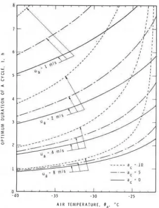
p i and Ah as 335 J/g, 0.91 Mg/m3 and 0.015 m, respectively, eqn. (13) (which is the criterion for the construction) requires QT to be 4.57 MJ/mZ. This QT value, as indicated in Fig. 2(b), corresponds to T = 4.7 h. The cycle is therefore to end at t = 4.7 h and the next flooding to be applied. The optimum condition is thus obtained in terms of the duration of a cycle for the particular meteorological conditions. The optimum duration of a cycle is presented in Fig. 3 for various meteorological conditions; some of the features are summarized below:
(1) The optimum duration, T, increases rapidly with increase in air temperature, decrease in wind speed, and increase in cloud.
- 4 0 - 35 - 3 0 - 2 5
A I R T E M P E R A T U R E . B a . " C
Fig. 3. Compiled chart of optimum length of time of flooding-and-freezing cycle for various meteorological condi- tions. QT is taken to be 4.57 MJ/mZ h, which corresponds to Ah = 0.015 m.
(2) For a given cloud cover, the effect of the air temperature increases with decrease in wind speed.
(3) When the air temperature is low, the wind speed is more important than cloud, the effect of which is almost negligible for high wind speeds. (4) As temperature increases, the effect of cloud
cover becomes increasingly significant.
(5) The effect of cloud cover for a given temperature increases rapidly as wind speed decreases.
DISCUSSION
Effect of layer thickness
An estimate of the optimum condition was made in the previous sections for a constant layer thick-
ness, Ah = 0.015 m, an average value encountered
in the field. Thickness, however, fluctuates, usually from flooding to flooding but also from location to
location within a flooded area. The Ah value is, so
long as the current procedure for flooding is followed (Baudais et al., 1974), within a range of about 0.01 to 0.02 m during most of the construction period.
The layer thickness Ah corresponding to QT is
plotted in Fig. 2 @) as a reference axis, indicating the
relation between Ah and T. Estimation of optimum
length of a cycle can also be obtained for a different layer thickness by means of the same procedure. The rate of heat loss or rate of increase in QT is larger in the earlier part of a cycle, as shown in Fig. 2(a and b). If a thinner water layer is applied, the growth rate of the ice platform is faster under the same meteorological conditions and the same
criterion. If Ah = 0.005 m, for example, QT being
1.52 MJ/mZ, T is about 1 h (see Fig. 2(b)). It would take only about 3 h, therefore, to build up 0.015 m of ice, whereas it would take 4.7 h if a layer of 0.015 m were applied in one cycle. This comparison may be exaggerated because eqns. (6-9) were ob- tained with layers of 0.01 to 0.02 m (Nakawo, 1980); it may have to be modified for layers as thin as 0.005 m. Taking this limitation into account it is still considered effective to reduce the layer thickness to establish a faster growth rate for a platform under given meteorological conditions and the proposed criterion.
238
OPTIMIZATION OF CRITERION TEMPERATURE constant value. Equation (13) requires
QT
to be equal to the total amount of heat released in freezingThe criterion temperature was taken to be -1.5'~ a flooded layer and bringing its temperature from
in the calculations shown in the previous section 0, to 8,. When ice is built up according to eqn. (13),
since the temperature at x = x, was observed to therefore, it is considered that layers with a tempera-
be about this value during an actual construction. ture of 8, are piled up successively just below the
Each flooding-and-freezing cycle was adjusted height corresponding to the current value of x,.
through the operator's estimate of the degree of The heat conduction equation was used to examine
solidification of the built-up ice (strength criterion). how the temperature profile, and hence the tempera-
That no accidents have occurred seems to justify this ture gradient, vary with time for x <x,.
procedure. In other words, -15°C may be an It was assumed, for simplicity, that the thermal
adequate value for 8,. diffusivity of natural and built-up sea ice is the same,
The criterion, however, may be too conservative being independent of temperature. The equation of
with regard to the strength of the ice, and a higher heat conduction is then given by
value could be taken for 0,. If - 1 0 " ~ is taken for
a2e
1ae
O,, for example, the same thickness of built-up ice - - - - 0 .
can be achieved more rapidly, or thicker ice can be ax2 K a t ('41)
made in the same period.
What should be the appropriate criterion tempera- the growth sea ice at the
ture? Only by optimizing it in relation to both the the is
total thickness of the platform and the mechanical = em at =
.
properties of the resultant ice can this question be (A2)
answered. The total thickness that can be obtained The initial condition would be expressed by the fol-
in the period available for constructing the platform lowing equations, assuming a constant temperature
can be predicted as a function of 8, by the use of 0, in the hypothetical built-up ice and a linear tem-
eqn. (13) and the data on general ambient conditions. perature profile in natural ice before construction
Future investigations are needed to establish the is started:
relation between ice quality and the criterion
temperature for construction.
e
= 8, where x>
d (A318 = y ( e c - e m ) x + 8 , w h e r e O < x < d (A4)
ACKNOWLEDGEMENTS d
0s - e m
The author is grateful to R. Frederking and L.E. with y =
-
e c - e m ('4.5)
Goodrich for their kind help in the preparation of this paper. It is a contribution from the Division of
These initial conditions are shown with solid lines in
Building Research, National Research Council of
Fig. Al, taking the values indicated in the Notation.
Canada, and is published with the approval of the
The solution of eqns. (Al) to (A4) is given by Director of the Division.
6 = (ec-em)
[
(yx +d)erf(s)
-APPENDIX 1 2d
x - d 2 6
Upward heat conduction from the bottom of an ice
-
(YX -d)erf(<) +(T)
sheet 2 d -
The criterion used to determine the duration of
1e.P -
(
]+ern
( ~ 6 )the flooding cycle is that the heat deficit of the layer
5 I ' 1
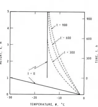
I I Temperature profiles are shown with dotted lines
I '
- 900
in Fig. A1 for various times after construction is
' t
.
9004
-
'J started. The temperature gradient is obtained by dif-1 h ferentiating eqn. (A6).
-
600 3 -ae
(0,-em,[
( x t d ) ( x d)
-
- -
X f y erf --
y erf-
1 % '-
ax 2d 2 L t 2 4 7 C I w-
-
300 u 2 - C t --- I % I* t \ \ * I I , % I t = O \ , \' \' 1 ,\ (A7) %.
,$-
0\I Assuming xc increases with time at the same rate
as the build-up rate of ice,
o x, = d - y t r t
-30 - 20 - 10 0 (A81
T E M P E R A T U R E . 8 , o c where
Fig. A l . Temperature profde at different times after con- y = h ~ - x , (A91
struction is started. The initial thickness (natural sea ice) is
taken to be 1 m. The right-hand ordinate corresponds to the Variation of the temperature gadient at x = xc
time when the built-up ice reaches a rriven hekht from the is obtained with the values given in the Notation by
bottom of the ice sheet.
-
- eqns. (A7) and (A8) for various values of y (Fig. A2).H E I G H T O F T O P S U R F A C E , h N , m
0 300 600 900 1 200 1 5 0 0
T I M E F R O M T H E B E G I N N I N G O F C O N S T R U C T I O N , t, h
Fig. A2. Variation of temperature gradient at different depths from the top surface. The upper abscissa corresponds to the height of the top surface of the built-up ice established at a given time. The right-hand ordinate shows the corresponding heat flux for a given temperature gradient.
The value of y was observed to be about 0.5 m
(Nakawo, 1980). The lines for y = 0 and 0.2 in Fig.
A2 are therefore meaningless, since eqns. (A6) and (A7) are applicable only for x
<
xc. For y in the range of 0.4 to 0.6 m, the temperature gradient increases asymptotically to zero; that is, the heatconducted upward at x = xc decreases with time,
approaching zero asymptotically (the scale is shown in the right-hand ordinate).
It decreased from 0.21 MJ/m2 h, which is the value corresponding to the temperature gradient in
the natural ice at t = 0, to about 0.03 MJ/m2 h in the
first 300 h. During this time about 1 m of ice was built up. The value of 0.03 MJ/m2 h at t = 300 h is small compared with the rate of heat loss at the surface during a flooding cycle (radiative heat flux is, for example, about 0.1 MJ/m2 h (Fig. 2(a)). As the rate of heat flow by conduction continues to decrease with time, it can be neglected in estimating the optimum flooding conditions, except for the earlier stage of construction.
During this period conductive heat may have to be taken into account. Equation (12) should then be used for the calculation rather than eqn. (13). Selec- tive deep flooding, however, is usually carried out in this early period in order to smooth the rough surface of natural ice (Baudais et al., 1974). The method of free floodings, as discussed in this paper, is applied afterwards. Early floodings, therefore, are outside the scope of this paper.
REFERENCES
Adams, Jr., C.M., French, D.N. and Kingery, W.D. (1960), Solidification of sea ice, J . Glaciol., 3 (28): 745-76 1. Ambach, W. and Hoinkes, H. (1963), The heat balance of alpine snow-field (Kesselwandferner, 3240 m, Oetztal Alps, August 11-September 8, 1958), Preliminary com- munication; Int. Ass. of Scientific Hydrology, Commis- sion of Snow and Ice, General Assembly of Berkeley, IAHS Publication No. 61, pp. 24-26.
Anderson, D.L. (1960), The physical constants of sea ice, Research, 13(3): 310-318.
Baudais, D.J., Masterson, D.M. and Watts, J.S. (1974), A system for offshore drilling in the Arctic Islands, J. Canadian Petroleum Technology, 1 3 (3): 15-26. Dykins, J.E. (1963), Construction of sea ice platforms, in:
Kingery, W.D. (Ed.), Ice and Snow, pp. 289-301.
Dykins, J.E. and Funai, A.I. (1962), Point Barrow trials - FY 1959; Investigations on thickened sea ice, U.S. Naval Civil Engineering Lab., Technical Report R 185.
Masterson, D.M., Anderson, K.G. and Strandberg, A.G. (1979), Strain measurements in floating ice platforms and their application to platform design, Canadian J. of Civil Engineering, 6(3): 394-405.
Nakawo, M. (1980), Heat exchange at a surface of a built-up ice platform during construction, Cold Regions Science and Technology, 3(4): 323-333.
Nakawo, M. and Frederking, R. (1981), The salinity of artificial built-up ice made by successive floodings of sea water, Proc. IAHR Int. Symp. on Ice Problems, Quebec City, 27-31 July, 1981, Vol. 11, pp. 516-524.
This publication is being d i s t r i b u t e d by the Division of Building R e s e a r c h of t h e National R e s e a r c h Council of Canada. I t should not b e r e p r o d u c e d i n whole o r i n p a r t without p e r m i s s i o n of the original publisher. The Di- vision would be glad to b e of a s s i s t a n c e i n obtaining s u c h p e r m i s s i o n .
Publications of the Division m a y b e obtained by m a i l - ing the a p p r o p r i a t e r e m i t t a n c e (a Bank, E x p r e s s , o r P o s t Office Money O r d e r , o r a cheque, m a d e payable to the R e c e i v e r G e n e r a l of Canada, c r e d i t NRC) t o the National R e s e a r c h Council of Canada, Ottawa. K1A 0R6. S t a m p s a r e not acceptable.
A l i s t of a l l publications of the Division is available and m a y b e obtained f r o m the Publications Section, Division of Building R e s e a r c h , National R e s e a r c h Council of Canada, Ottawa. KIA OR6.