Bubble Behavior in Subcooled Flow Boiling on Surfaces of Variable Wettability
by
Emily W. Tow
Submitted to the
Department of Mechanical Engineering
in Partial Fulfillment of the Requirements for the Degree of
Bachelor of Science in Mechanical Engineering
at the
Massachusetts Institute of Technology
June 2012
ARCHIVES
MASSACHUSETTS INSTITUtEf OF TECHNOLO3YJUN 2
8 2012
LIBRARI ES
@ 2012 Massachusetts Institute of Technology. All rights reserved.
Signature of A uthor...
Department of Mechanical Engineering May 11, 2012
Certified by... .. ... ... .
<9
Evelyn N. WangAssociate Pro o echanical Engineering The1:1sis 'r
Accepted by... ...
I im-. MEEK arV Samuel C. Collins echanical Engineering
Bubble Behavior in Subcooled Flow Boiling on Surfaces of Variable Wettability
by
Emily W. Tow
Submitted to the Department of Mechanical Engineering on May 11, 2012 in Partial Fulfillment of the Requirements for the Degree of
Bachelor of Science in Mechanical Engineering
ABSTRACT
Flow boiling is important in energy conversion and thermal management due to its potential for very high heat fluxes. By improving understanding of the conditions leading to bubble departure, surfaces can be designed that increase heat transfer coefficients in flow boiling. Bubbles were visualized during subcooled nucleate flow boiling of water on a surface of variable wettability. Images obtained from the videos were analyzed to find parameters influencing bubble size at departure. A model was developed relating the dimensions of the bubble at departure to its upstream and downstream contact angles based on a rigid-body force balance between momentum and surface tension and assuming a skewed truncated spherical bubble shape. Both experimental and theoretical results predict that bubble width and height decrease with increasing flow speed and that the width increases with the equilibrium contact angle. The model also predicts that the width and height increase with the amount of contact angle hysteresis and that the height increases with equilibrium contact angle, though neither of these trends were clearly demonstrated by the data. Several directions for future research are proposed, including modifications to the model to account for deviations of the bubbles from the assumed geometry and research into the parameters controlling contact angle hysteresis of bubbles in a flow. Additionally, observations support that surfaces with periodically-varying contact angle may prevent film formation and increase the heat transfer coefficients in both film and pool boiling.
Thesis Supervisor: Evelyn Wang
ACKNOWLEDGEMENTS
I would like to acknowledge several people whose assistance with this research was
indispensable to me. First, I must thank my thesis advisor, Professor Evelyn Wang, who
provided critical guidance on my research direction. I would like to thank Siyu Chen for working
closely with me and performing contact angle and contaminant analysis, Kuang-Han Chu, Ryan
Enright, and Professor TieJun Zhang for their help with the planning and execution of this
research, and Rong Xiao and Solomon Adera for teaching me to use the lab equipment. Finally, I
would like to thank the Air Force Office of Scientific Research (AFOSR) and Battelle for
funding this work.
TABLE OF CONTENTS
Acknowledgements
3
List of Figures
5
List of Tables
6
1. Introduction
7
2. Background
9
3. Methods
17
3.1 Experimental Apparatus
17
3.2 Video Collection
21
3.3 Experimental Parameters
23
3.4 Data Extraction
24
4. Results and Discussion
27
4.1 Bubble Departure
27
4.2 Observations
44
4.3 Evaluation of Experimental Fixture
49
5.
Conclusion
57
6. References
59
Appendix I: All Departing Bubbles on Contaminated Surface
60
LIST OF FIGURES
2.1 Regions of film boiling in a vertical tube 11
2.2 Contact angle for liquid-vapor-solid interfaces 12
2.3 Flow-direction rigid-body force balance on a bubble 15
3.1.1 Schematic of the experimental apparatus 17
3.1.2 Sample holder 19
3.1.3 Schematic of channel 20
3.1.4 Thin film gold heater on the back of the surface 21
3.4.1 Series of video frames that indicate the premature departure of a bubble 24 3.4.2 MATLAB script inputs for calculation of channel height, bubble width, and
downstream and upstream contact angles 25
3.4.3 MATLAB script inputs for calculation of bubble height for an image with known
channel height 26
4.1.1 A bubble before and after departure from the surface 28
4.1.2 Bubbles in a variety of sizes and shapes 28
4.1.3 Downstream contact angle plotted against upstream contact angle 29
4.1.4 Contact angle difference plotted against bubble width 30
4.1.5 Water droplet on the contaminated surface during contact angle measurement 31 4.1.6 Water droplet on a smooth silicon surface during contact angle measurement 31 4.1.7 Contact angle measurements of the contaminated surface 32
4.1.8 Plot of width vs. height for all departing bubbles 33
4.1.9 Bubble width at departure is compared to average contact angle 34 4.1.10 Bubble width is compared to downstream and upstream contact angles 35 4.1.11 Bubble height at departure is compared to average contact angle 36 4.1.12 Bubble height is compared to downstream and upstream contact angles 37
4.1.13 Bubble height is plotted against flow speed 38
4.1.14 Theoretical bubble width is compared to the data 40
4.1.15 Theoretical bubble height is compared to the data 41
4.1.16 Bubbles at the moment before departure with overlays of the assumed bubble shape 42
4.2.2 Bubble changing shape rapidly before departure 45
4.2.3 A triangular bubble 46
4.2.4 Consecutive images of a bubble showing a rapid change in shape when jumping
over a hydrophilic region 47
4.2.5 Hypothetical surface with periodic variations in wettability 48 4.2.6 Bubble that may be trapped in a small hydrophobic area within a hydrophilic region 49
4.3.1 Examples of clear video stills 50
4.3.2 Examples of unclear video stills 51
4.3.3 Consecutive images of a departing bubble which show that video frame rate should
be increased 53
4.3.4 Used plain silicon surface showing visual evidence of contamination 54 4.3.5 An XPS test of the contaminated wafer surface. 55
LIST OF TABLES
1. INTRODUCTION
This work aims to inform the design of microstructured surfaces for higher heat fluxes in
flow boiling for applications in thermal energy conversion and thermal management. Flow
boiling-and boiling in general-are heat transfer processes of great importance to current
technology because of the very high heat transfer coefficients that can be achieved.
High heat fluxes are needed in the thermal management of microprocessors as their
transistor density grows. As Gordon Moore predicted in 1965, the number of transistors on
individual integrated circuits has roughly doubled every two years [1]. However, the increasing
transistor density and number of interconnect layers has increased the heat generation per unit
area and therefore the necessary heat flux out of the chip. Recently, finned aluminum or copper
heatsinks have become insufficient, and heat pipes in combination with fins have been used to
more effectively remove heat. The heat removed from the chip by a heat pipe is limited by the
critical heat flux (CHF) of the surface-fluid combination. Currently, most heat pipes use pool
boiling to begin heat removal from the chip. However, the heat flux can be increased by
increasing the speed of the flow past the heated surface, so flow boiling may be the future of
thermal management. Although we do not consider the CHF in flow boiling, similar ideas may
be involved in extending the region of nucleate boiling to higher vapor qualities in order to
increase the heat flux for a given heater temperature.
Microstructured surfaces that exhibit complete wetting and are rough have been shown to
increase the CHF in pool boiling over smooth surfaces [2]. Because flow boiling is directional
and the forces governing the departure of the bubbles are different, the effectiveness of the same
surfaces is unknown in flow boiling. For this reason, the original goal of this research was to
evaluate in flow boiling the same microstructured surfaces that had been so successful in pool
boiling. These surfaces consisted of an array of micro-scale pillars which in this case created a
superhydrophilic surface. The roughness of the surfaces may also augment boiling heat transfer.
Following the decision to not make new microstructured surfaces this year and the
discovery of contamination in the experimental fixture, a new experimental procedure
materialized. Plain surfaces were observed to take on a widely-varied wettability upon
contamination by particles in the fixture, and this property was exploited in order to compare the
bubble size at departure to the surface wettability. Bubble departure was studied by capturing
images of bubbles in flow boiling and comparing the size at departure to the local surface contact angles and fluid flow speed.
2. BACKGROUND
Flow boiling is heat transfer from a surface to a moving liquid which causes it to change
to vapor phase. As the fluid progresses either through a channel or across a hot structure, the
fluid increases in quality (defined as the vapor mass to total mass ratio) and the fluid and thermal
interactions go through many stages. For the many applications of flow boiling, increasing the
boiling heat flux for a given wall temperature is often useful. By examining the parameters that
govern the heat flux, which in all but the latest stages of flow boiling occurs through the
generation of bubbles, it may be possible to design surfaces and geometries that improve the
performance of systems that use boiling.
Boiling is an excellent form of heat transfer because of the very high heat fluxes that can
be achieved with normal materials and relatively small temperature differences. In any kind of
boiling-pool boiling, in which the water is stagnant on the heater, or flow boiling, in which
convection with the heater is forced-heat conducts through the water near the surface and
locally heats it to above the saturation temperature. At a suitable nucleation site, that superheated
water evaporates, becomes a growing bubble. When the bubble departs from the surface, it
disrupts the water around it, allowing cold water to come near the surface where it heats up. By
constantly moving the water, the bubbles in boiling allow the conduction distance through the
water to be very short, greatly lowering the thermal resistance (compared, for example, to
conduction or natural convection without boiling) and increasing the heat transfer coefficient.
However, the bubbles themselves are made of very low-conductivity vapor and any area of the
surface that is covered at a given time by bubbles is a region that is not releasing much heat.
Therefore, understanding the interactions between bubbles and the surface in boiling is key to
improving heat fluxes in boiling.
In pool boiling, much research is in progress on increasing the critical heat flux (CHF).
CHF occurs in pool boiling when the rate of bubble nucleation increases so much that film
boiling begins. In film boiling, the bubbles form a film of gas through which the dominant mode
of heat transfer is generally radiation. The thermal resistance of the gas film is greater than that
of conduction through water in nucleate boiling, so the heat flux out of a hot object (such as a
microprocessor) begins to decrease if the heat generation is unchanged. This causes the
temperature to rapidly increase until the radiant heat flux eventually surpasses the CHF, at which
point the surface is so hot that most metal parts will have melted. Theoretical correlations that predict the CHF, such as Equation 1, generally predict it independently of surface conditions:
4 ,= Khg [pg , -p,), (1)
where
4i..is
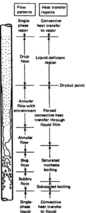
the CHF, K is a geometric constant, u- is fluid surface tension, g is gravitational acceleration, and pf and pg are densities of the liquid and gas, respectively [3]. However, recent research has shown that hydrophilic microstructured surfaces can substantially increase the CHF [2]. Using microfabrication to create very hydrophilic surfaces that encourage bubbles to depart earlier, leaving a greater contact area between the hot surface and the water, can achieve an increase in the CHF [2].CHF applies to pool boiling only, but the coalescence of bubbles into a film is likely to impair heat transfer in flow boiling as well. Flow boiling is more complicated, with the boiling type and heat flux varying with, wall temperature fluid velocity, and quality. Figure 2.1 shows the regions of flow and heat transfer behavior in flow boiling in vertical tubes.
Flow Heat transfer patterns region$s 0 '
6
L:
Single- Convective phase heat transfer vapor to vaporDrop Uquld deficie
renion nt On~ Annular flew with entrainment Forced convective heat transfer through liquid film Annular flow Slug Saturated flow nucleate boiling Bubbly flowI I Sub 9 *dboiling Single-phase liquid vout point Convective heat transfer to liquid
Figure 2.1. Regions of film boiling in a vertical tube with flow from bottom to top. Image adapted with permission from A Heat Transfer Textbook by J. H. Lienhard IV and J. H. Lienhard V [4].
Flow boiling looks different depending on the steam quality, wall temperature, and boiling geometry. For instance, flow boiling in a horizontal tube or channel, such as the one used in this experiment, will exhibit different multi-phase flow behavior than what is shown in Figure
2.1, above. However, in any geometry, the earliest (lowest-quality, and therefore occurring at the beginning of the heated region) regions of flow boiling involve individual, quasi-spherical bubbles. As shown in Figure 2.1, this region is called bubbly flow. The first part of bubbly flow is classified as subcooled boiling because some of the fluid has not yet risen to saturation temperature, but boiling can still occur because the water near the heater surface is above saturation temperature. The boiling analyzed in this work is subcooled boiling at a low heat flux, where the fluid bulk temperature has not reached saturation temperature and bubbles are sparse.
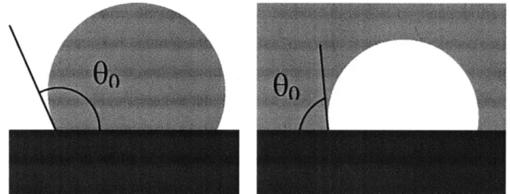
An important characteristic of a surface in boiling is its wettability by the fluid, which is quantified by the contact angle between the fluid and the surface in the presence of the fluid's vapor. The contact angle is the angle formed by the surface and the plane tangent to the surface of the fluid at the intersection with the surface. Around a bubble, the contact angle is again (in this work) taken to be the contact angle of the fluid with the surface. When the fluid is water and the contact angle is less than 90*, leading to flat droplets and round bubbles, the surface is considered to be hydrophilic. When the contact angle is more than 900, round droplets and flat bubbles form, and the surface is considered hydrophobic. Figure 2.2 illustrates the contact angle for a droplet and a bubble.
Figure 2.2. Contact angle for liquid-vapor-solid interfaces: a droplet on a hydrophobic surface (left) and a bubble on a hydrophilic surface (right).
Drops and bubbles form the shapes they do because each interface has surface energy. The equilibrium contact angle is reached when the total surface energy of the liquid-gas-solid system is minimized on a surface normal to the direction of gravity. Young's equation gives the
Ysv -YSL = y COs
( 2
where ysL and ysv are the surface energies of the solid-vapor and solid-liquid interfaces,
respectively, and y is the surface tension (or surface energy) of the liquid interfacing with its own
vapor [5].
For a droplet on a tilted surface, the contact angle is not constant around the contact line.
As the tilt is increased, the maximum angle around the droplet increases and the minimum
decreases. The maximum angle when the droplet begins to slide is called the advancing contact
angle and the minimum is called the receding contact angle. When the equilibrium contact angle
is not known, it can be approximated to be a weighted average of the advancing and receding
contact angles,
6Rand
OA,respectively, as given by Equations 3 through 5 [5].
00
= arccoS]FA COS OA + FR COSOR where (3)TA + TR ,wer
TR
~Sin
3 OR 134
(2-3cosOR
+ OR 3c andFA Sin3 OA A )1/3(5
2-3cos6A2+cos3
-The equilibrium contact angle is a weighted average because of the cosine in Equation 2
and the nonlinear (to state the obvious) dependence of cosO on 0.
Knowing the contact angles allows for the estimation of the balance of forces that
prevents a bubble from departing. S.G. Kandlikar found expressions for the forces on a bubble
that lead to departure in subcooled flow boiling based on forces due to surface tension,
buoyancy, drag, pressure difference, and momentum changes [6]. These expressions assume a
truncated-spherical bubble geometry for the momentum and drag calculations and a two-part
geometry for the surface tension, buoyancy and pressure difference calculations. They also
assume low flow velocity and a constant wettability surface. For this paper, a simpler model will
be developed using the contact angles and bubble height measured and only considering the
surface tension and momentum change forces. Kandlikar also does not assume the bubble is a
rigid body, which the model here will. Kandlikar makes the important distinction that the
advancing and receding contact angle of a droplet on a surface are not equivalent to the upstream
and downstream contact angles of the water around a bubble in a flow because the advancing and
(2)receding are the maximum and minimum contact angles and the upstream and downstream angles lie between those values [6]. In this paper, the local equilibrium contact angle of the surface will be estimated to be the average of the upstream and downstream contact angles as measured at the moment before departure.
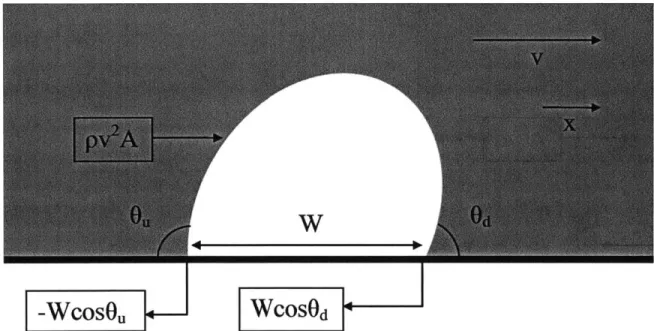
This work will estimate the bubble dimensions at departure based on a rigid-body force balance in the direction of fluid flow. The flow-direction force balance is assumed to dictate the departure rather than the forces normal to the surface. Only two forces will be considered: the force in the direction of the flow (the x-direction) due to the change in momentum of the water behind the bubble and the force in the negative-x-direction due to the x-component of the surface tension around the bubble. Shear forces and the force due to the pressure drop in front of the bubble are neglected in this analysis. Viscosity-driven pressure drop along the length of the channel is also neglected.
The force of the water behind the bubble will be found via conservation of momentum, assuming that the x-direction momentum goes to zero for the fluid over the area of the bubble as projected in the plane perpendicular to x. For this calculation, the bubble is assumed to take the shape of a sheared truncated sphere, which has a truncated circle for a flow-direction cross-section and a circle for a contact area. The heated region of the channel is not beyond the fluid entry length so a parabolic laminar flow profile cannot be assumed, and the presence of other bubbles in the channel makes the velocity profile almost impossible to predict. For simplicity, the fluid velocity is assumed to be in the x-direction only and the profile is assumed to be constant throughout the channel, except when encountering the bubble in question. Steady-state conservation of momentum states that the net force in the x-direction, F., on a control volume is related to the net momentum flux out of the control volume, as given in Equation 6. p is the water density, i' is the water velocity, and v_ is the x-component of velocity, where v,, and vx,,, denote the velocity entering and exiting the control volume, respectively. Based on the assumptions given above, vx,. is equal to the bulk water velocity, v, and v,, is zero. Therefore,
F =fpvXv -*=dA= p -v =-pv2A (6) The net force in the x-direction on the water behind the bubble is found to be -pvA, which is equal and opposite to the force exerted on the bubble by the water, pv2A. This force should take the form of a pressure difference between the water behind and in front of the
The surface tension force is assumed to be equal to that of a bubble with a square base of side length equal to the diameter of the circle where the bubble contacts the surface. The edges of the square that are parallel to the flow will not contribute to the x-component of the force, and the upstream and downstream edges are assumed to contact the surface at the upstream and downstream contact angles, respectively. These x-direction surface tension forces are equivalent to those on a bubble with a circular base where the front half of the bubble contacts the surface at the downstream contact angle, Od, and the back half at the upstream contact angle, 0..' The surface tension forces, along with the force of the water behind the bubble, are shown graphically in Figure 2.3.
-WCOSu
WCOSOd
Figure 2.3. The flow-direction force balance on a bubble in a left-to-right flow. Forces are given in the direction of arrows, not necessarily in the x-direction. The subscripts u and d denote upstream and downstream, respectively.
The length in the direction of flow that the bubble contacts the surface will be called the width, denoted as Win Figure 2.3 and in the following equations. The force balance illustrated in Figure 2.3 leads to the following equation:
pv2A =W(cos9 -cos9.) (7)
where A is the projected area perpendicular to the direction of the flow. This force balance will
be true at all times, not just at the moment before departure. Departure will occur at a critical
moment where one term changes and the other cannot, such as when one or both of the contact
angles reach the advancing or receding contact angles of the fluid-vapor-surface combination.
The shape projected in the x-direction is assumed to be a truncated circle with contact
angles 0a equal to the average of the upstream and downstream contact angles. For angles in
radians, the area and radius, r, are given by Equation 8 and 9.
A = 7r (l+- +r2 cos 6 sin , where (8)
r = 2n (9)
2sin O
Substitution of Equations 8 and 9 into Equation 7 results in a force balance as a function
of W:pvW
2cs~)(04si 2w (; - .a + cosOa sinOa)= oW(cos6d - COS ,) (10)
4
Sin 26.Solving for W leads to the following equation for bubble width at departure as a function
of the upstream and downstream contact angles:
40-(cosOd -cos0.) sin2 Oa
pv ; -Oa + cos Oa sinOa , where 60 +6.
6, = "
(12)
Assuming again that the bubble's x-direction projected area is a truncated circle, the
bubble's height, H, can be found from the width and average contact angle with Equation 13:
(1_+
COS ,2a-(cosOd
- cos 0.) sin Oa(1+ cos Oa) (13)2 sin0. pv 2 --0a +cos Oa sin Oa
where 0
3. METHODS
3.1 Experimental Apparatus
In this experiment, deionized and degassed water is boiled on flat silicon surfaces in forced convective flow. The experimental fixture allows for the collection of video of bubbles in flow boiling. The bubbles are viewed from the side with a microscope to capture the upstream and downstream contact angles. A pump pushes water through a preheater which brings the water to near saturation temperature and a small heater on the back side of the silicon surface initiates boiling, which is captured by the camera. The fluid cools through a heat exchanger, completing the loop. Figure 3.1.1 shows a schematic of the experimental apparatus.
Figure 3.1.1. A schematic of the experimental apparatus. Water flow lines are indicated by bold arrows. The numbered elements are described in detail in the text below.
Figure 3.1.1 shows the setup of the experimental apparatus. Numbered elements are detailed in the following list:
1. Peristaltic pump: Cole-Parmer #7553-70, 6-600 rpm with Masterflex Easy-Load II
head #77200-62 and Masterflex size 15 silicone tubing.
2. Pulse dampener: Cole-Parmer #07596-20. Trapped (easily compressible) air absorbs pulses of fluid from peristaltic pump for more even flow through the channel.
3. Flowmeter: Omega FLR 1000-ST.
4. Preheater: copper coiled tube, 1/4" ID, 2.7 m long, heated by 30.5 K coiled wire heater controlled by Variac transformer #TDGC-2KM which outputs 0-130 VAC at 60Hz.
5. Thermocouple: Omega thermocouple read by Stanford Research Systems #SR630 16
channel thermocouple monitor.
6. Channel: 0.67 mm x 4.65 mm x 20mm minichannel housed in sample holder. See Figures 3.1.2 and 3.1.3 below for details.
7. Heater: 1 mm x 1 mm gold deposited resistive heater with resistance of 163 9 controlled by a 25V power supply. Typically 8-10 V was used.
8. Heat exchanger: Lytron #631OG3SB copper tubing with Mechatronix fan #UF25GC12.
9. Differential pressure transducer: Setra #2301005PD2F2DB. Senses 0-5 PSID. Data from this sensor was not collected or used in this experiment, but could be used in future research.
10. Microscope: Nikon Eclipse #TE2000-U at 10x*1.5x magnification with mercury lamp controlled by X-cite Series 120.
11. Camera: Vision Research model Phantom v7.1 with Phantom camera control software.
All elements were connected by tubing of silicone and an unknown plastic using stainless steel and brass compression fittings. Various parts of the fixture were sealed with silicone RTV.
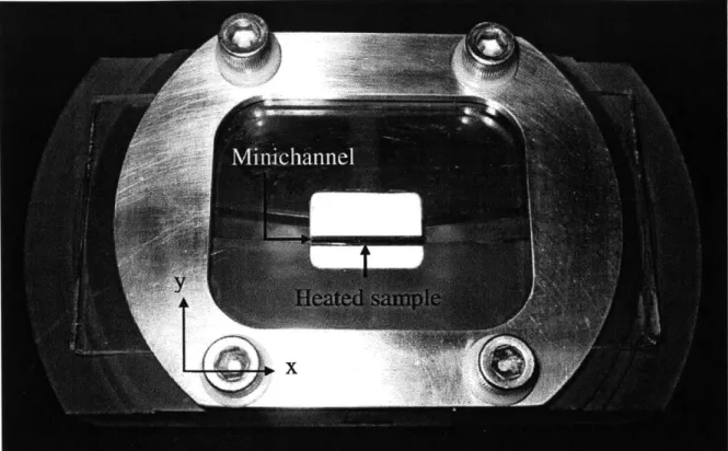
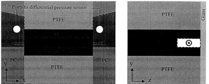
The silicon minichannel is housed in a sample holder made of polycarbonate (PC) with Teflon (PTFE) spacers holding the channel in place. A glass front plate is held on by bolts and
Figure 3.1.2. A photograph of the sample holder with the channel and heated surface indicated by arrows. Water enters and exits from the back. x and y directions are given to clarify Figure 3.1.3, which shows a schematic of the channel.
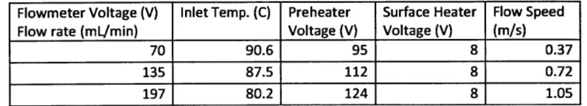
Figure 3.1.2 shows the sample holder and indicates the channel and the heated sample where boiling occurs. Water enters and exits from the back. The minichannel consists of three squares of silicon sandwiched between two PTFE blocks. The glass plate forms the front wall. A schematic of the channel is shown in Figure 3.1.3 below.
Figure 3.1.3. The channel is shown schematically from the front (at left) and from the side, looking through the channel (at right). The channel is outlined with a dashed line and arrows indicate the direction of flow. The bottom silicon piece contains the heater and the surface of interest. The transition from the PC channel to the silicon minichannel is abrupt. The eddies that are likely to form there may obscure the pressure readings, which were not collected for this analysis. The right-handed x, y and z coordinates relate this schematic to the photograph in Figure 3.1.2.
As shown in Figure 3.1.3, the channel is a silicon sandwich in which the bottom piece contains the heater and the surface of interest. Water flows from the larger PC channel to the thinner and shallower silicon channel. The transition from the PC channel to the silicon channel is abrupt. The eddies that are likely to in the transition region may obscure the pressure readings, which were not collected for this analysis. However, this may cause problems in future research using this same fixture.
The sample itself has two sides, on one a smooth and (initially) clean silicon surface and on the other a deposited gold resistive heater. Figure 3.1.4 shows the heater on the back side of the surface.
Figure 3.1.4. The thin film gold heater on the back of the surface. The pale square at the top of the gold pattern is the heating element, which has a resistance of 163 A.
The heater itself is 1mm x 1mm and has a resistance of 163 2. The round gold pads allow spring-loaded electrodes to apply power from the 25V (max) power supply. The sample and other silicon pieces are cut from a 15 cm diameter, 0.675 mm thick silicon wafer.
Before data collection, the fixture is cleaned with deionized water. The sample and other silicon parts are cleaned with methanol, isopropyl alcohol, and deionized water (in that order) and dried under a nitrogen gas flow. Then the sample is plasma cleaned in oxygen for 15 minutes and installed in the fixture.
3.2 Video Collection
In this experiment, information is gained by analyzing video of the bubble nucleation, growth and departure as a function of surface wettability and water flow rate. After the surface is prepared and installed, the system is filled with degassed water and closed. For each of three flow rates, video of the bubbles in the channel is recorded while the system is in steady state.
First, the prepared sample and other parts are inserted into the clean sample holder. The heater electrodes are screwed in and electrical continuity is confirmed. The glass, which has been is plasma cleaned with oxygen for 15 minutes to improve wettability, is placed over the open channel under a slow flow of DI water to minimize the amount of air trapped under the glass.
The glass is attached with screws and the sample holder is attached to the rest of the fixture with
compression fittings.
Water is boiled on a hot plate in 1L Erlenmeyer flasks to remove dissolved gas. The
water is cooled in air to
55C
to prevent damage to the flowmeter. This water is then introduced
into the system just upstream of the pump to flush the existing water, which may contain
dissolved gas, out. Some air is allowed to remain in the pulse dampener to absorb the pulses of
fluid that come from the pump. When the system is filled with degassed water, it is closed by
connecting the outlet and inlet via compression fittings under a bowl of degassed water. In
practice, not all air is removed from the system, but this method seems to minimize it.
The pump, preheater and heat exchanger fan are turned on and the water temperature
begins to rise. The preheater voltage is controlled manually using optical feedback from the
microscope until the water exiting the preheater reaches steady state at the highest possible
temperature that does not cause bubbles of dissolved air to nucleate in the microchannel. The
pressure in the channel is approximately atmospheric but the exact pressure is not known. The
surface heater is turned on at 6V and then the voltage is raised until a reasonable rate of
nucleation is reached in the center of the channel, around 8-10V. The fixture position is adjusted
to record the farthest- upstream nucleation sites, rather than those closest to the heater, in order to
avoid premature departure due to jostling from bubbles that have already departed upstream. The
microscope is focused on the bubbles and then switched to the camera, which has been turned
on. The mercury lamp is turned on, the reflective light turned off, and the microscope refocused
for the camera based on the preview on the computer screen. The lamp brightness, microscope
aperture and camera exposure are adjusted to obtain the best picture of the nucleating bubbles,
especially of their contact points with the surface.
Bubble video is recorded at three flow rates for each surface. The minimum is the
smallest flow rate that produces reasonably steady flow and small enough bubbles that clear
video can be recorded. The maximum would be the greatest flow rate that could be heated by the
preheater to a temperature where bubbles will nucleate in the channel, but in practice it is the
largest flow rate that can be heated without making the preheater insulation give off fumes.
When the system is running in steady state and the video preview is clear, video is
recorded at 30 frames per second at a resolution of 600x800 pixels. Greater resolution in time
being collected, the flow rate is observed in LabVE1W and the channel inlet temperature is recorded. Video collection is stopped after six minutes (the largest possible duration allowed by the camera for the given resolution and frame rate) and the fixture is brought to equilibrium for the next test flow rate while the video compiles.
After recording videos at all flow rates, the entire fixture except the pump and fan are turned off. After the preheater has cooled enough to prevent pool boiling, the pump and fan are shut off.
3.3 Experimental Parameters
Video was collected for two surfaces: one that was clearly contaminated from use in evaluation of the fixture performance and for a short time in air and one that was oxygen plasma cleaned the day of the video collection. The freshly-cleaned one quickly became contaminated during flow boiling testing. Because the second surface became contaminated and because the
video quality was inferior, no data analysis was performed from the video of boiling on the second surface. Only the video of the first contaminated surface was used for data analysis.
Video was collected of the contaminated surface in flow boiling with the experimental parameters given in Table 1.
TABLE 3.3.1. Experimental parameters for evaluation of flow boiling on the contaminated surface. Flowmeter Voltage (V) Inlet Temp. (C) Preheater Surface Heater Flow Speed Flow rate (mL/min) Voltage (V) Voltage (V) (m/s)
70 90.6 95 8 0.37
135 87.5 112 8 0.72
197 80.2 124 8 1.05
Flow speed was calculated from the flowmeter voltage and channel dimensions. Inlet temperature was determined such that the frequency of bubble departure in the channel was moderate. The inlet temperature is significantly lower than the saturation temperature of water at atmospheric pressure because of the presence of dissolved air in the water despite attempts to remove it. Thus, the bubbles that form are likely to contain a mixture of air and steam, but the forces that govern the bubbles and their shape and size at departure should be very nearly equivalent to those which govern bubbles of steam in boiling.
3.4 Data Extraction
Bubble size and contact angle were found for bubbles in the moment before departure from the surface with a MATLAB script involving clicking at predetermined places in stills extracted from the boiling videos.
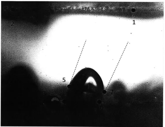
Video was reviewed to find bubbles at the moment before departure. Changes in the surrounding bubbles were observed to determine whether the bubble departure was due to the forces exerted on it by the flow and the surface or due to a collision or coalescence with another bubble. An example of a bubble that clearly did not depart of its own accord is given in Figure 3.4.1.
Figure 3.4.1. An example of a series of video frames which indicate that the departure of a bubble was premature and thus should not be used in data analysis. In this case the bubble appears to have been pushed off by another bubble, as indicated by the shadow in the central image.
The shadow in the middle image of Figure 3.4.1 is probably that of some larger bubbles which were generated in the preheater and entered the channel. Shadows like this were a clear indication that any bubbles departing at that time should not be analyzed. The bubbles around the departing bubble were also examined to determine the reason for departure. If bubbles upstream of the bubble in question or bubbles on the opposite side of the channel also departed or changed shape or size at the same time, none of the bubbles departing at that time were considered. Pictures were extracted just before the departure of bubbles that departed on their own. Pictures were also taken of other interesting bubble phenomena.
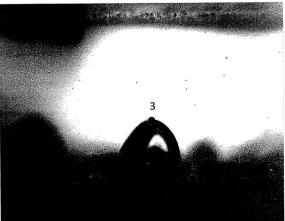
For departing bubbles, a MATLAB script was written to find the bubble width (the length, in the direction of flow, of the contact area of the bubble with the surface) and downstream and upstream contact angles. Points of interest were clicked on with position information recorded by the built-in function ginput. The sequence of clicks, shown in Figure 3.4.2, was repeated three times and averaged to reduce human error.
Figure 3.4.2. The inputs into the MATLAB script for calculation of channel height, bubble width, and downstream and upstream contact angles. Point 3 was placed at whichever point on the top surface was clearest.
The 21 clicks that made up three full cycles of seven spatial inputs were averaged to get the seven points shown in Figure 3.4.2. Bubble width and contact angles, as well as the channel width in pixels, were calculated by the script based on the averaged inputs. The channel width in pixels was compared to the known channel width of 0.67 mm to find the sizes in mm of other bubble dimensions.
A separate but similar function was used to find the bubble height-the maximum dimension perpendicular to the surface-for a picture with a known mm-to-pixel ratio. The sequence of clicks used to find the height is shown in Figure 3.4.3. As before, three cycles of inputs were averaged before being used to find the height.
Figure 3.4.3. The inputs into the MATLAB script for calculation of bubble height for an image with known channel height.
The second script is separate because the decision to measure bubble height came later. If this experiment were to be repeated, it would be beneficial to combine the two scripts. Both scripts are included in Appendix II.
Bubble height, width, and downstream and upstream contact angles are poor measures compared to volume and contact area, which cannot be found because the bubble dimensions perpendicular to the plane of the video are unknown. The dimensions that were measured will, however lend some insight. Further study will have to determine the effects of bubble width,
4. RESULTS AND DISCUSSION
4.1 Bubble Departure
Bubble dimensions at departure were collected from video images and compared to the measured contact angles and theoretical predictions for bubble size. A great variety of bubbles were observed, and in all relationships there is a fair amount of scatter. The experimental data shows that bubble width-that is, the length of surface in the direction of flow that is touched by the bubble-increases with equilibrium contact angle and decreases with flow speed. Bubble height (in the direction perpendicular to the surface) is found to decrease with flow speed but show little relationship to contact angle. Theoretical results are shown to have moderate agreement with experimental results, indicating that both width and height decrease with flow speed and increase with equilibrium contact angle and contact angle hysteresis. These results will be detailed in this section.
Stills taken from the flow boiling video give downstream and upstream contact angles and bubble width and height at the moment before departure. Since the video frame rate was 30 frames per second, the bubble size may have been recorded up to 33.3 ms before the actual departure, but because low heat fluxes were used the bubbles grew slowly (over seconds to tens of seconds) and the size difference between the final picture before departure and the actual moment before departure should be minimal. The surface tested was contaminated such that the wettability was not constant, so by comparing the size of the bubble to the local wettability, as estimated by the average of the downstream and upstream contact angles.
The video quality was variable, but the view of the growing and departing bubbles was clear most of the time. Many factors, which will be discussed in detail later, stood in the way of getting clear numerical data from the departing bubbles. Of the 30 minutes of boiling video collected, 25 departing bubbles at three flow rates were clear enough to use in this analysis. Figure 4.1.1 shows one departing bubble.
100 pm
Figure 4.1.1. A bubble before (left) and after (right) departure from the surface.
Several types of bubbles formed on the contaminated surface. Figure 4.1.2 shows four bubble types that were observed with a variety of sizes and contact angles.
Figure 4.1.2 depicts four types of bubble shapes that were observed. Additionally, Appendix I shows images of all departing bubbles. With so many bubble shapes, the relationship between downstream and upstream contact angle in the bubbles observed is weak, as shown in Figure 4.1.3. 180 h 160 140 -to C 120 - O0
9
Up - 0em.37 m/s 0 0 E 80 A 0 0.72 m/s M 60 - O O 40. - )A1.05 m/s 0 20-0. 0 20 40 60 80 100 120 140 160 180 Upstream Contact Angle (deg)Figure 4.1.3. Downstream (water) contact angle is plotted against upstream contact angle, with bubbles shown representing the three main regions of the plot.
As would be expected for a surface with relatively constant wettability within the region of a bubble, the downstream angle generally increases with increasing upstream angle. However, there is a great spread. The downstream contact angle is generally smaller than the upstream contact angle, consistent with expectations for bubbles in a flow. The contact angles vary for a given flow rate, indicating that the surface has non-uniform wettability. The amount of contact angle hysteresis also varies for a given flow rate, indicating that the wettability variation occurs on a small enough length scale that a single bubble can span multiple zones of wettability. There is also no clear trend in the amount of contact angle hysteresis between the three flow rates, as shown in Figure 4.1.4, which follows.
120.00 -0 100.00 U O O -a 80.00 -CD Um 60.00 -
A
0 nO0.37 mn/s CDO0 00.72 m/s 40.00 0 00 <00
A1.05 m/s 20.00 -A
00
U O 0.00 0. )0 0.20 0.40 0.60 0.80 1.00 1.20 -20.00 Bubble Width (mm)Figure 4.1.4. The contact angle difference is plotted against width for the three flow rates, showing no trend in either set of variables and indicating that the variation in contact angle due to the surface wettability non-uniformity is greater than the variation in contact angles due to the different flow rates used.
The average difference between the upstream and downstream contact angles was 48.9 degrees with a standard deviation of 30.9 degrees.
The contact angle of a still droplet on the contaminated surface was measured using a goniometer. Figure 4.1.5 shows a small water drop on the contaminated surface that was used in the contact angle measurements.
10 pm
Figure 4.1.5. A water droplet on the contaminated silicon surface during contact angle measurement. The average maximum contact angle at the location tested was 145.30.
Contamination made the silicon surface hydrophobic, as demonstrated by the obtuse contact angle in Figure 4.1.5, above. The contamination can be clearly seen on the surface. This wafer had originally been cleaned with solvents and then plasma-cleaned with oxygen, but contamination resulted from the use of the wafer in the flow-boiling fixture. A freshly plasma-cleaned silicon surface is shown in Figure 4.1.6.
Figure 4.1.6. A water droplet on a smooth, oxygen plasma-cleaned silicon surface during contact angle measurement. The average maximum contact angle was 39.10.
The low contact angle between the water and the smooth silicon surface shows that the smooth, oxygen plasma-cleaned surface is hydrophilic, in stark comparison to the contaminated surface. The mirror-like finish shows the absence of contamination and surface defects on the surfaces before they are contaminated during use in the fixture.
The contact angle measurements of drops on the contaminated surface, taken shortly after the collection of flow boiling video, are shown in Figure 4.1.7.
160 150 140 Uo S130 120 (U 110 0 U 100 90 80 1 0 5 10 15 20 Time (s) 25 30 35 40
Figure 4.1.7. Contact angle measurements of the contaminated surface, average peak of 145.3*. The six lines represent six series of measurements.
showing an
The average maximum contact angle was 145.3 degrees, showing the contaminated surface to be hydrophobic. The standard deviation in maximum contact angle was 1.4 degrees, which is small compared to the distribution in average contact angle seen in the flow boiling video (see Figure 4.1.3). However, the contact angle measurements were all taken at the same location, so only a small variation would be expected. The contact angle of the drop first increases with time while the drop reaches equilibrium and then decreases gradually as the (very small) drop evaporates. The maximum contact angle generally corresponded with the maximum
to be the equilibrium contact angle. Because these contact angle measurements were all taken at the same location, the variability is contact angle over the contaminated surface was not demonstrated. On average, the equilibrium contact angle of all bubble departures recorded on the contaminated surface was 106.70.
Although the original goal of this research was to use several surfaces of different (but constant) wettability, the variable-wettability surface as useful in that it allowed for the examination of bubble departure at many average contact angles on a single surface.
Having examined the wettability of the contaminated surface and found it to be generally hydrophobic but highly variant, the size of the bubbles can be discussed in comparison to the contact angles observed. A variety of bubble sizes and shapes were observed at the moment before departing from the surface. Figure 4.1.8 shows that both the width and the height of the bubbles were highly varied.
0.6 -0.5 -E0.4
-.6.0
0
0~
0.3 - 0 0 0.37 m/s O 00.72 m/s .a 0 1 0.~ OAOA
A
A 1.05mr/sA A
A
0.1 -0I i I 1 1 0.00 0.20 0.40 0.60 0.80 1.00 1.20 Bubble Width (mm)Figure 4.1.8. The width and height of all departing bubbles are plotted, showing the variation in bubble size and the dependence on flow rate of bubble height.
The departing bubbles range from 0.13 to 0.52 mm in height 0.15 to 1.04 mm in width2.
Figure 4.1.8 shows that for the surface tested, bubble height at departure is inversely related to liquid flow rate regardless of contact angle. The dependence of the bubble width on flow rate is not clear because of the range of contact angles and the strong dependence of bubble width on average contact angle, which is shown in Figure 4.1.9, which follows.
1.20 1.00 -EE 0.80 O E M 0.37 m/s - 0 0.72 rn/s 0.60 0 A 1.05 rn/s --- Linear (0.37 m/s) S0.40 - A A A A Linear (0.72 m/s) Linear (1.05 m/s) 0.20 - 0 0.00 50.00 70.00 90.00 110.00 130.00 150.00 170.00 Avg. Contact Angle (deg)
Figure 4.1.9. Bubble width at departure is compared to average contact angle at three water flow rates, given as the bulk velocity of the water in the channel. For each flow rate, the bubble width increases with increasing contact angle. At a given contact angle, lower flow rates produce wider bubbles. Linear fits were applied to the data to show the general trend in bubble width with contact angle, but there is insufficient data to determine if the relationship is linear.
Figure 4.1.9 shows that the bubble width at departure is positively correlated with the average contact angle and inversely correlated with the flow speed. The average (taken over the three flow rates) increase in bubble width is 0.011 mm per degree of water contact angle. This
means that if wider bubbles enhance flow boiling, more hydrophobic surfaces should be employed, and hydrophilic surfaces should be used if narrower bubbles improve boiling.
Bubble width was also compared to the downstream and upstream contact angles to determine if one mattered more, but the results were not enlightening. Figure 4.1.10 shows that although the trend of width vs. contact angle is still generally increasing, the results are more scattered than those with the average contact angle.
1.20 1.00 E E 0.80 0.60 3 0.40 0.20 0.00 0
0
MA
O.37 m/s 00.72 m/s - 0 l A 1.0! 0.00 100.00Downstream Contact Angle (deg)
5 m/s E -0I .0 m 1.20 -1.00 -0.80 -0.60 -0.40 -0.20 -0.00 A 0
* 4
OIO
N
0.37 m/s 00.72 m/s A1.Os m/s 0.00 100.00Upstream Contact Angle (deg)
Figure 4.1.10. Bubble width is compared to downstream (at left) and upstream (at right) contact angles, but neither correlation is stronger than that with average contact angle.
Bubble width increases with both downstream and upstream contact angle, though it appears to be more strongly correlated with average (or equilibrium) contact angle.
Bubble height was also measured, and is plotted against average contact angle in Figure 4.1.11.
0.6 -0.5 -0.4 E bb 0 0.3 - O O *0.37 m/s O0 00.72 m/s .A U.5 0.2 -A A1.05 m/s
A A
A
0.1 -50.00 70.00 90.00 110.00 130.00 150.00 170.00 Avg. Contact Angle (deg)Figure 4.1.11. Bubble height is compared to average contact angle. For each flow rate, bubble height appears to be relatively constant across all contact angles. However, the dependence of height on flow rate is striking. Faster flows clearly lead to shorter bubbles.
According to Figure 4.1.11, bubble height is strongly correlated with flow rate (or flow speed) but shows almost no correlation with contact angle. As with the bubble width, comparing the height to the downstream and upstream contact angles separately yields no new information, but will be included here for completeness. Figure 4.1.12 shows these comparisons.
0.6 -E0.5 -E
~0.4
- U W+ 0.3 - OO O O 0.37 m/s 0.2 - 00.72 m/s .0A 0.1 A 1.05 m/s 0 0.00 100.00Downstream Contact Angle (deg)
E. E .0 .0 0.6 0.5 -0.4 0.3 0.2 0.1 -U 9 M
0
A
0.37 m/s 00.72 m/s A 1.05 m/s 0.00 100.00Upstream Contact Angle (deg)
Figure 4.1.12. Bubble height is compared to downstream (at left) and upstream (at right) contact angle to see if the effect of one is greater. These show the same inverse correlation of height with flow rate but all plots show no obvious relationship between bubble height and contact angle.
Comparisons of height to the downstream and upstream contact angles individually show the same inverse correlation of height with flow rate but still show no obvious correlation between bubble height and contact angle. In all likelihood, the relationship was to average contact angle is clearer because the wettability is so varied on the surface that the average contact angle was a better predictor of local wettability than either the downstream or upstream contact angles.
Figure 4.1.13 plots height against flow speed without regard to contact angle and shows the inverse correlation.
0.6 0.5 E 0.2 90.2 0.1 y = -0.3373x + 0.5261 R2=0.59 0
08
0*
1 1 1 1 I 0.0000 0.2000 0.4000 0.6000 0.8000 1.0000 1.2000 Flow Speed (m/s)Figure 4.1.13. Bubble height is plotted against flow speed, showing the decreasing relationship.
Height is clearly dependent on flow speed in this experiment: the minimum, maximum, and average height all decrease monotonically with flow speed. The variation in height also appears to decrease with bubble height. There is too much scatter to determine the shape of the correlation, but for a linear fit the bubble height can be estimated to decrease by 0.38 mm per m/s of fluid speed.
By affecting the wettability, contamination increased the bubble sizes at departure over the clean surface. Contamination gave the surface a greater variability in contact angle but on average made the surface more hydrophobic. The contaminated surface had an average contact angle of 106.73 compared to 39.1* for a smooth, plasma-cleaned surface. A first-order approximation which assumes a linear relationship between contact angle and bubble width of 0.01127 mm/degree, as found from the data in Figure 4.1.9, shows that the bubbles on the contaminated surface should be 0.76 mm wider on the contaminated surface than on the equivalent surface without contamination. Given that the average width of all departing bubbles analyzed in this experiment was 0.50 mm, that difference is significant. Clearly the average bubble departing from a smooth, oxygen plasma-cleaned silicon surface would not be negative,
as the estimated change in width would suggest. There are many variables and uncertainties that limit the usefulness of this estimation, but the point is that the magnitude of the possible change in bubble size due to contamination is significant compared to the magnitude of the bubbles. Therefore, contamination can greatly affect the bubble size in a boiler. Assuming that bubble width (and/or contact angle) has some effect on heat flux, contamination will have a great effect on the performance of a boiler. This effect may be amplified in micro- and nano-structured surfaces, whose usefulness may be compromised by even a small amount of contamination.
A theoretical model was developed relating bubble dimensions at departure to the upstream and downstream contact angles. The contact angles will be extracted from the experimental results to find the theoretical departure size. The theoretical results are calculated from Equations 11 through 13 and are compared to the measured results.
In calculating the theoretical bubble dimensions, the following values of surface tension and density were used. The surface tension of water in contact with air at 100*C is taken to be 0.0598 N/m [7]. This value of surface tension is not entirely accurate for this experiment because of the mix of steam and air in the bubbles and the range of temperatures at which nucleation occurred (see Table 3.3.1), but it will be fairly close to the actual values for the bubbles recorded. The water density, again at 1000C, is taken to be 958.4 kg/m3 [8].
First, the bubble width at departure was evaluated theoretically based on the measured contact angles and the flow speed. The measured and theoretical results for all bubble widths are plotted together in Figure 4.1.14 to show the agreement of the model with the observed behavior.
2.0 1.8 -1.6 -E 1.4 1.2 -1.0 - A Bubbles 0.8 - Linear (Bubbles) 0 0.6 -
A
0.4 -A 0.2-A
A
A
0.0 0.0 0.2 0.4 0.6 0.8 1.0 1.2 1.4Measured Bubble Width (mm)
Figure 4.1.14. Theoretical bubble width is compared to the data. The theoretical width is based on the measured upstream and downstream angles of the bubbles recorded at departure. Though there is a lot of scatter, the linear fit of the model versus the data is very close to the 1:1 line, showing a reasonable level of agreement between the model and the data.
The theoretical model generally predicts the measured bubble width well, though there is a lot of scatter. A linear fit of the theoretical to the measured bubble width almost exactly matches the 1:1 line drawn between the model and data. This is good, but the scatter indicates that for a given bubble, the model will not necessarily predict the width at departure with accuracy. This suggests that there are factors excluded by the model that affect the bubble width at departure. One bubble was excluded from the plots in Figures 4.1.14 and 4.1.15 which had an upstream contact angle greater than its downstream contact angle, leading to negative theoretical width and height.
The bubble height at departure was also predicted theoretically for the measured contact angles. This comparison, which shows a more marked discrepancy between the model and data,
0.9
-A
0.8 -0.7 -E E 0.6 -0.5 -A Bubbles c 0.4 -- 1:01A
- Linear (Bubbles) 0.3 -0A
"0.2 0.1 - 0-0 0.1 0.2 0.3 0.4 0.5 0.6 0.7Measured Bubble Height (mm)
Figure 4.1.15. Theoretical bubble height is compared to the data. The agreement is fairly good though there is a shift of about 0.15 mm between the measured and theoretical bubble height, with the theory predicting shorter bubbles than were actually observed. This is probably due to the assumption that each bubble was a skewed truncated sphere, a shape which did not always accurately describe the bubbles observed.
The theoretical and measured bubble height appear to be better correlated than the theoretical and measured bubble width, but there is a clear shift between the two values. The measured bubble height seems to be about 0.15 mm larger than that predicted by the model. This is likely to be due to the assumption that the bubbles are skewed4
truncated spheres. The projected area in the plane of the images captured would then be a skewed truncated circle, but this is generally not the case. In almost all cases, the bubble was taller than it would have been if it had formed a truncated circle between the two points of contact with the same contact angles.
4 Skewing a sphere (in this case, in the direction of flow) affects neither its volume nor its projected area
Figure 4.1.16 shows two examples of real bubbles overlaid with skewed circles to show the discrepancy.
Figure 4.1.16. Two bubbles at the moment before departure with overlays of the assumed bubble shape shown by a dotted line. Bubbles were assumed to be skewed truncated spheres with a truncated skewed circle for a cross section. In both cases, as it seems to be in all images taken of bubbles the moment before departure, the bubble is taller than would be predicted by the truncated skewed sphere model.
Bubbles were assumed to be skewed truncated spheres, with the cross section in the plane of the video being a truncated skewed circle. In almost all (or perhaps all) images taken of bubbles the moment before departure, the bubble was taller than would be predicted by the truncated skewed sphere model. This helps explain the discrepancy between the measured and theoretical data, in which the measured height is generally greater than the predicted height.
Deviations of the model from the data may originate from several other assumptions that are not entirely accurate. Assuming that the liquid behind the bubble lost all x-direction velocity, neglecting shear, and neglecting pressure changes between the bulk fluid and the fluid in contact with the bubble is inaccurate, and should be replaced by a drag force that depends on the size and shape of the bubble and the velocity profile in the channel. Additionally, it was assumed that departure is governed by an imbalance in forces in the flow direction, but it is possible that for some bubbles departure was triggered by forces in the direction normal to the surface. Employing a drag force and determining whether and when bubbles depart due to a force


![[PDF] Document de formation pour débuter la programmation Smartphone Android par la pratique - Free PDF Download](data:image/gif;base64,R0lGODlhAQABAIAAAP///wAAACH5BAEAAAAALAAAAAABAAEAAAICRAEAOw==)