No title

(1)

HAL Id: hal-02957292

https://hal.archives-ouvertes.fr/hal-02957292

Submitted on 8 Oct 2020

HAL is a multi-disciplinary open access

archive for the deposit and dissemination of

sci-entific research documents, whether they are

pub-lished or not. The documents may come from

teaching and research institutions in France or

abroad, or from public or private research centers.

L’archive ouverte pluridisciplinaire HAL, est

destinée au dépôt et à la diffusion de documents

scientifiques de niveau recherche, publiés ou non,

émanant des établissements d’enseignement et de

recherche français ou étrangers, des laboratoires

publics ou privés.

N. Huneeus, O. Boucher, F. Chevallier

To cite this version:

N. Huneeus, O. Boucher, F. Chevallier. No title. Geoscientific Model Development, European

Geo-sciences Union, 2009, 2, pp.213-229. �10.5194/GMD-2-213-2009�. �hal-02957292�

(2)

www.geosci-model-dev.net/2/213/2009/

Geoscientific

Model Development

Simplified aerosol modeling for variational data assimilation

N. Huneeus1, O. Boucher2, and F. Chevallier1

1_{Laboratoire des Sciences du Climat et de l’Environnement, L’Orme de Merisier, Gif sur Yvette, France} 2_{Met Office, Hadley Centre, Exeter, UK}

Received: 28 May 2009 – Published in Geosci. Model Dev. Discuss.: 23 June 2009

Revised: 4 September 2009 – Accepted: 10 September 2009 – Published: 16 November 2009

Abstract. We have developed a simplified aerosol model

to-gether with its tangent linear and adjoint versions for the ulti-mate aim of optimizing global aerosol and aerosol precursor emission using variational data assimilation. The model was derived from the general circulation model LMDz; it groups together the 24 aerosol species simulated in LMDz into 4 species, namely gaseous precursors, fine mode aerosols, coarse mode desert dust and coarse mode sea salt. The emis-sions have been kept as in the original model. Modifications, however, were introduced in the computation of aerosol opti-cal depth and in the processes of sedimentation, dry and wet deposition and sulphur chemistry to ensure consistency with the new set of species and their composition.

The simplified model successfully manages to reproduce the main features of the aerosol distribution in LMDz. The largest differences in aerosol load are observed for fine mode aerosols and gaseous precursors. Differences between the original and simplified models are mainly associated to the new deposition and sedimentation velocities consistent with the definition of species in the simplified model and the simplification of the sulphur chemistry. Furthermore, sim-ulated aerosol optical depth remains within the variability of monthly AERONET observations for all aerosol types and all sites throughout most of the year. Largest differences are ob-served over sites with strong desert dust influence. In terms of the daily aerosol variability, the model is less able to re-produce the observed variability from the AERONET data with larger discrepancies in stations affected by industrial aerosols. The simplified model however, closely follows the daily simulation from LMDz.

Sensitivity analyses with the tangent linear version show that the simplified sulphur chemistry is the dominant process responsible for the strong non-linearity of the model.

Correspondence to: N. Huneeus

(nicolas.huneeus@lsce.ipsl.fr)

1 Introduction

Aerosols play an important role in atmospheric physics and chemistry through their impact on pollution, actinic fluxes, visibility, acid rain, and climate. Numerous atmospheric models include a representation of aerosols aimed at simulat-ing their physical and chemical properties such as their con-centration, size distribution, chemical composition, and state of mixture. However, the uncertainties about their emissions result in a wide range of uncertainties about their overall im-pact on climate (Forster et al., 2007). Large diversity ex-ists among global aerosol models for desert dust and sea salt mainly due to the differences in the parametrization of their source fluxes and particle size. Sulphate, particulate matter and black carbon present smaller diversity due to the use of similar data sets for emission (Textor et al., 2006). Neverthe-less, the uncertainty remains large.

Traditionally, emissions have been estimated through bottom-up techniques which integrate source information across sectors. However, top-down techniques have been de-veloped in recent years that exploit the combination of satel-lite data and numerical models through inverse techniques. An important technique for this purpose is variational data assimilation. It allows obtaining an optimal state estimate by finding the best compromise between background informa-tion and observainforma-tions. Robertson and Langner (1998) suc-cessfully applied this method to estimate the source intensity of an inert gas. Since then it has also been applied for the esti-mation of the emission of other gaseous species (e.g. Cheval-lier et al., 2005; Stavrakou and M¨uller, 2006; Elbern et al., 2007; Meirink et al., 2008; Chevallier et al., 2009; Kopacz et al., 2009). However its application to estimating aerosol and/or aerosol precursor emissions remains limited. Hakami et al. (2005) assimilated black carbon concentration from ob-servations to retrieve its emission and initial condition over eastern Asia using the adjoint of the Sulphur Transport Eu-lerian Model (STEM). Yumimoto et al. (2007, 2008) esti-mated the emissions for an extreme dust event over Asia on April 2005 and reproduced the exercise for a dust event late

(3)

March and early April 2007. In both works lidar observations were assimilated to the Regional Atmospheric Modeling System/Chemical Wheather Forecasting System 4-D varia-tional data assimilation system (RAMS/CFOR-4DVAR). On a global scale and using a variational-like method, Dubovik et al. (2008) estimated the emissions of fine and coarse mode aerosols for a period of two weeks during August 2000. In their study MODIS (Moderate Resolution Imaging Spectro-radiometer) aerosol optical depth (AOD) at 550 nm was as-similated into the Goddard Chemistry Aerosol Radiation and Transport (GOCART) model. Henze et al. (2009) assimi-lated ground measurement from the Interagency Monitoring of Protected Visual Environments (IMPROVE) network to estimate aerosol precursor emissions and used the results to quantify their influence on representative air quality metrics. Models of different level of complexity are used when conducting variational data assimilation on multiple aerosol species. While models of high complexity faithfully repre-sent the known physical and chemical processes, simplified models and those of intermediate complexity have the ad-vantage of focusing on important processes and of render-ing the simulations computationally efficient and conceptu-ally easier to understand. Henze et al. (2004) and Sandu et al. (2005) developed inverse box models of aerosol dynam-ics that focus on the physical particle dynamdynam-ics with lim-ited chemical and thermodynamic transformations. Zhang et al. (2008) used an aerosol model with a simplified aerosol representation in the first attempt to operationally assimilate aerosols into the Naval Research Laboratory (NRL) numeri-cal weather prediction (NWP) system. An aerosol model was developed and introduced into the Integrated Forecast Sys-tem (IFS) of the European Centre of Medium Range Weather Forecast (ECMWF) to assimilate satellite aerosol products into a NWP model for reanalysis and forecast (Morcrette et al., 2009; Benedetti et al., 2009).

In this paper we present a simplified aerosol model that simulates AOD from emission fluxes of the main aerosol species and gaseous precursors. The model has been de-signed with the aim to estimate the intensity of the aerosol emissions through variational data assimilation of daily av-erages of AOD. As a consequence the tangent linear and ad-joint versions of the new model have also been developed. Applications of this aerosol model to variational data assimi-lation will be presented in a forthcoming article. We structure this paper as follows. We start by presenting the general cir-culation model used to set up the simplified model (Sect. 2). We continue by presenting the simplified model and validate it with respect to the original model and surface measure-ments from the AErosol ROobotic NETwork (AERONET; Holben et al., 1998) (Sect. 3). We then present its tangent linear and adjoint version (Sect. 4). The linearity and sen-sitivity of the forward model will also be analysed in this section. Finally, Sect. 5 presents the conclusions and per-spectives of this work for estimating aerosol source intensity.

2 Reference general circulation model

The general circulation model of the Laboratoire de M´et´eorologie Dynamique (LMDz) in its version 3.3 sim-ulates the global life cycle for the main aerosol species, namely sea salt (SS), desert dust (DD), organic matter (OM), black carbon (BC) and sulphate (SU). Its standard version has a resolution of 3.75◦ in longitude, 2.5◦in latitude, and 19 levels in the vertical with a hybrid σ -pressure coordinate with five of its levels under 850 hPa and nine above 250 hPa. The model computes the atmospheric transport with an Eu-lerian finite volume transport scheme for large scale advec-tion, a turbulent mixing scheme within the boundary layer and a mass flux scheme for convection. The time step for the dynamics equations is three minutes. The mass fluxes are accumulated over 5 time steps in order to apply the large scale advection every 15 min. The physical and chemical parametrisation are applied every 30 min. An operator split-ting technique is applied to the different processes that affect the prognostic variables (Boucher et al., 2002).

The sulphur cycle includes six sulphur species: dimethyl-sulfide (DMS), sulphur dioxide (SO2), hydrogen sulfide (H2S), dimethylsulfoxide (DMSO), methanesulfonic acid (MSA) and sulphates (SU). These last two species are as-sumed to be in the particulate phase. The sulphur emis-sions from fossil fuel combustion and industrial processes are taken from the EDGAR version 3.0 database (Olivier and Berdowski, 2001), from which a fixed 5% from combus-tion sources is assumed to be emitted directly as sulphate. An additional source of sulphur is the antropogenic emis-sion of H2S. For the natural emissions we take the same sul-phur emissions as those described in Boucher et al. (2002). Annual emission rates are 66.3 Tg S/yr for industrial SO2, 2.82 TgS/yr for H2S, 4.8 TgS/yr for continues volcanic erup-tions and 19.4 TgS/yr oceanic emissions of DMS. The bio-genic emissions of DMS and H2S over continents are 0.31 and 0.51 TgS/yr, respectively, and the biomass burning emis-sions of SO2 are 2.99 TgS/yr. The sulphur chemical cy-cle considers the sulphate production in both gaseous phase, through the oxidation of SO2by the hydroxyl radical (OH), and aqueous phase, through the oxidation of SO2by ozone (O3) and hydrogen peroxide (H2O2). A full description of the sulphur cycle and its validation can be found in Boucher et al. (2002) and Boucher and Pham (2002).

The model considers 10 sea salt bins with radii between 0.03 µm and 20 µm and 80% relative humidity (RH) (0.03– 0.06 µm, 0.06–0.13 µm, 0.13–0.25 µm, 0.25–0.5 µm, 0.5– 1.0 µm, 1.0–2.0 µm, 2–5 µm, 5–10 µm, 10–15 µm and 15– 20 µm). The mass emission for each bin is calculated with the source formulation of Monahan et al. (1986) according to the wind at 10 m.

Desert dust emissions follow Schulz et al. (1998) and Guelle et al. (2000). To take into account the horizontal wind variability and the strong dependence of the dust emis-sions on wind, the emisemis-sions are pre-calculated off-line at a

(4)

higher resolution (1.125◦_×_1.125◦_{) using the 6-hourly}

hor-izontal 10-m wind speeds analyzed at ECMWF. They are then regridded to the LMDz resolution (3.75◦_×_2.5◦_{) while}

conserving the global mass. The model considers only two modes of dust aerosols: fine particles with radius between 0.03 and 0.5 µm and coarse particles with radius between 0.5 and 10 µm (Reddy et al., 2005).

Organic matter is emitted as organic carbon (OC) with a conversion rate of 1.4 and 1.6 for fossil fuel and biomass combustion, respectively. The OC emissions from biomass burning are calculated considering an OC to BC ratio of 7. The emissions of BC due to biomass burning are taken from Cooke and Wilson (1996), whereas the emissions of both BC and OC from fossil fuel combustion are taken from Cooke et al. (1999). Another source of OC is the condensation of volatile organic compounds (VOCs). These are represented in the model as terpenes. The conversion from terpenes to OC can vary largely depending on factors such as the initial concentration of terpenes, whether the oxidation is started by O3or OH, and the ratio between hydrocarbons and nitrogen oxides (NOx). The OC production rate from the emission of terpenes is taken as 11% in LMDz. The model makes the difference between hydrophilic and hydrophobic OM and BC. It simulates the aging process for these particles through a conversion from hydrophobic to hydrophilic particles with an exponential lifetime of 1.63 days.

The model considers the processes of dry and wet deposi-tion as well as sedimentadeposi-tion. Dry deposideposi-tion is calculated as a function of the concentration in the lowest level and a de-position velocity (Tables 1 and 2). This dede-position velocity is taken constant for the different types of surface considered. The model does not differentiate between hydrophilic and hydrophobic particles of OM or BC when calculating dry de-position. Wet deposition is split between in-cloud and below-cloud scavenging and hydrophobic and hydrophilic particles are treated differently in below-cloud processes. The sedi-mentation is calculated by LMDz in terms of a sedisedi-mentation velocity. This velocity depends on the dry aerosol diameter, the atmospheric conditions of temperature and pressure for the desert dust, and the dependence of size to relative humid-ity for sea salt aerosols.

For the optical properties the same configuration as in Reddy et al. (2005) is taken. Aerosols are described as an external mixture. Their optical properties such as single scat-tering albedo (ω), mass extinction coefficient (αe) and the

asymmetry factor are computed using the Mie theory and prescribing the refractive indexes.

3 Simplified aerosol model

3.1 Forward model

The forward model (H ) computes the observations (y) from the input parameter (x). In this work y is taken to be the total

and fine mode AOD fields whereas x is the emissions of the main aerosol species and aerosol precursors and the chemical lifetime of precursor gases, expressed as

y = H (x) (1)

The model H corresponds to a reduced aerosol model (hereafter referred to as SPLA) derived from the general circulation model LMDz described in the previous section. Modifications were introduced only in the aerosol module, the meteorology and transport are the same as LMDz. The main simplification is the reduction of the scheme from 24 original species into 4 species. These are the gaseous aerosol precursors, the fine mode (or accumulation mode) aerosol, the coarse mode desert dust aerosols and the coarse mode sea salt aerosols. The gaseous aerosol precursor vari-able groups together DMS, SO2and H2S. The aerosol fine mode includes SU, BC, OM, DD with radius between 0.03 and 0.5 µm and SS aerosols with radius smaller than 0.5 µm. The coarse DD mode corresponds to particles with radius between 0.5 and 10 µm whereas the SS coarse mode groups together particles with radius between 0.5 and 20 µm. The emissions from the original model are mapped onto the new set of variables with the total mass of aerosol precursor and aerosol emitted being the same.

The original oxidation pathways in gaseous and aqueous phases for the sulphur chemistry are reduced into one oxida-tion mechanism. The gaseous precursors are oxidized as a function of a lifetime representative of the oxidation of DMS and SO2. The production of sulphate (PSU) for each time

step 1t is:

PSU=[P G] (1 − e−1t /τchem) (2)

where [P G] is the concentration of precursor gases and τchem [days] is the chemical lifetime of precursor gases estimated through:

τchem=8 − 5cosθ (3)

where θ is the latitude in radians. The lifetime τchemvaries from 3 days in the Equator to 8 days in the poles. This choice was taken in order to best reproduce the columns of precur-sors and fine mode aerosols in LMDz. No seasonal or height dependence was introduced in the computation of this chem-ical lifetime.

The parametrisation of dry deposition is the same as in the original model; changes were introduced in the deposition velocities in order to adapt them to the new set of species. The new deposition velocities in SPLA for each one of the species are presented in Table 3. Over the ocean, the depo-sition velocities for the precursor gases (species 1) were cal-culated as the average of the deposition velocities of DMS and SO2weighted by their surface concentration. However, over continental surfaces, SO2 velocity was considered for specie 1 since this gas predominates in terms of concentra-tion over the other gases considered. In the same way, the

(5)

Table 1. Dry deposition velocities [cm/s] for each type of aerosol and all surfaces considered in LMDz. The velocities are the same for

hydrophilic and hydrophobic BC and OM. DD1corresponds to the desert dust particles with radius between 0.03 and 0.5 µm, whereas DD2 corresponds to particles with radius between 0.5 and 10 µm.

DMS SO2 SO4 H2S DMSO MSA H2O2 BC OM DD1 DD2

Ocean 0 0.7 0.05 0 1 0.05 1 0.1 0.1 0.1 1.2

Sea Ice 0 0.2 0.25 0 0 0.25 0.04 0.1 0.1 0.1 1.2

Land 0 0.3 0.25 0 0 0.25 1.5 0.1 0.1 0.1 1.2

Land Ice 0 0.2 0.25 0 0 0.25 0.04 0.1 0.1 0.1 1.2

Table 2. Dry deposition velocities [cm/s] for the 10 sea salt bins (SS1to SS10) and for all surfaces considered in LMDz. The corresponding particle radii are from 0.03 to 0.06, 0.06 to 0.13, 0.13 to 0.25, 0.25 to 0.5, 0.5 to 1.0, 1.0 to 2.0, 2 to 5, 5 to 10, 10 to 15 and 15 to 20 µm (sizes are for 80% RH).

SS1 SS2 SS3 SS4 SS5 SS6 SS7 SS8 SS9 SS10 Dep. vel. 0.1 0.1 0.1 0.1 0.1 1.2 1.2 1.2 1.5 1.5

Table 3. Dry deposition velocities [cm/s] for each tracer and each surface type in SPLA. Tracer 1 groups the gaseous precur-sors, namely DMS, SO2, and H2S. Tracer 2 represents the fine mode aerosols: SU, BC, OM and DD aerosols with radius between 0.03 and 0.5 µm and SS particles with radius smaller than 0.5 µm. Tracer 3 corresponds to the coarse DD aerosols with radius between 0.5 and 10 µm. Finally, tracer 4 groups the SS bins having radius between 0.5 and 20 µm.

Tracer 1 Tracer 2 Tracer 3 Tracer 4

Ocean 0.28 0.28 1.2 1.2

Sea Ice 0.2 0.17 1.2 1.2

Land 0.3 0.14 1.2 1.2

Land Ice 0.2 0.17 1.2 1.2

deposition velocity over ocean for specie 2, i.e. fine mode aerosols, is calculated as the weighted average of the veloci-ties of each one of the species considered in specie 2 (i.e. SU, BC, OM, DD and SS aerosols with a radius smaller than 0.5

µm). The dry deposition over the continents is calculated considering the concentrations and the deposition velocities over land and applying the same procedure as over ocean. The deposition velocity over sea and land ice corresponds to an average of the velocity of sulphate and the remaining com-ponents of species 2 over the same surfaces. Species 3 is the same as the one used in LMDz, therefore the deposition flux of specie 3 is equivalent to the second dust bin in LMDz. Fi-nally, for species 4, we have considered a deposition velocity of 1.2 cm s−1corresponding to a weighted average velocity for sea salt bins with radius between 0.5 and 20 µm.

In terms of wet deposition, the distinction between hy-drophilic and hydrophobic aerosols was eliminated. The dis-solution constant in in-cloud scavenging processes for fine mode aerosols (species 2) was set to the corresponding value of SO4used in LMDz, whereas for the coarse modes (both desert dust and sea salt) the same constant value of 0.7 is used as in the original model.

The sedimentation in SPLA is only applied to coarse desert dust (species 3) and sea salt aerosols (species 4). It is parametrized, as in LMDz, as a function of a mass median di-ameter. This parameter was adjusted in SPLA as to minimize the differences in burden of desert dust and sea salt between SPLA and LMDz. The mass median diameter of sea salt was taken as 90% of the value corresponding to a size distribu-tion between 0.5 and 20 µm and a RH of 80%, whereas for the desert dust, the mass median diameter used corresponds to one of a size distribution between 0.5 and 10 µm. Tables 4 and 5 give the values used in LMDz and SPLA, respectively. The model computes total and fine mode AOD at three wavelengths, namely 550, 670 and 865 nm. The AOD is cal-culated, like in LMDz, as the vertical integral of the product of the mass extinction coefficient, calculated off-line, and the mass of the corresponding aerosols species. For our species 2 (fine mode aerosols) the mass extinction coefficient (αe<2>) is calculated from the sulphate (αSO4) extinction coefficient,

which is a function of RH and wavelength (λ), and scaled to the mass of ammonium sulphate as follows:

αe<2>(RH,λ) = αSO4(RH,λ)

MSO4

M(NH4)2SO4

(4)

where MSO4and M(NH4)2SO4are the molecular masses of

(6)

Table 4. Mass median diameter (MMD, µm) for each bin of DD and SS used in the parameterisation of sedimentation in LMDz.

DD1 DD2 SS1 SS2 SS3 SS4 SS5 SS6 SS7 SS8 SS9 SS10

MMD 1 11 0.09 0.19 0.38 0.75 1.5 3.0 7.0 15 25 35

For the coarse mode desert dust (species 3), the unit mass extinction coefficient considers a size distribution equivalent to the one used in the original model and is calculated as follows: αe<3>(λ) = rmax R rmin σe(r,λ)n(r)dr rmax R rmin ρn(r)dr (5)

where rminand rmaxare the lower and upper limits, respec-tively, of the desert dust size distribution (0.5 and 10 µm, respectively), n(r)dr is the number of particles with a radius between r and r+dr, ρ the density of the particles and σeis

the mass extinction coefficient of desert dust.

Finally, the coarse mode of sea salt (species 4) groups the original sea salt bins with radius between 0.5 and 20 µm. The mass extinction coefficient (αe<4>) is calculated as the weighted average of the extinction coefficient for each bin in the original model:

αe<4>(RH,λ) = jmax P j =jmin αje(RH,λ)Bj jmax P j =jmin Bj (6)

where jminand jmaxcorrespond to the range of bin indices in LMDz considered for our species 4, Bj is the globally and annually-averaged burden of each bin j and αej is the mass

extinction coefficient of bin j .

3.2 Validation of forward model

We explore the performance and fidelity of SPLA by compar-ing it with AOD AERONET data and LMDz outputs. The analysis will be focused on the AOD at 550 nm. Further-more, the fidelity of SPLA in reproducing the aerosol cycle of emission, transport, deposition and sedimentation will be indirectly evaluated by comparing the burden between the two models.

3.2.1 Validation of SPLA with LMDz

We start by comparing SPLA against LMDz with respect to the burden for each one of the species defined in SPLA and we then extend the comparison to the AOD at 550 nm. The advantage of this approach is that it allows identifying pos-sible errors in the AOD as being due to errors in the aerosol

Table 5. Mass median diameter (MMD, µm) for tracers 3 and 4 in

SPLA used in the parameterization of sedimentation. Tracer 3 Tracer 4

MMD 12.7 2.8

cycle or in the computation of the AOD itself. Outputs of LMDz are grouped in the same way species are constructed in SPLA in order to make results comparable.

Aerosol burden

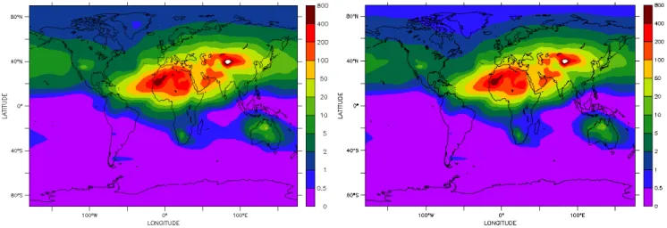
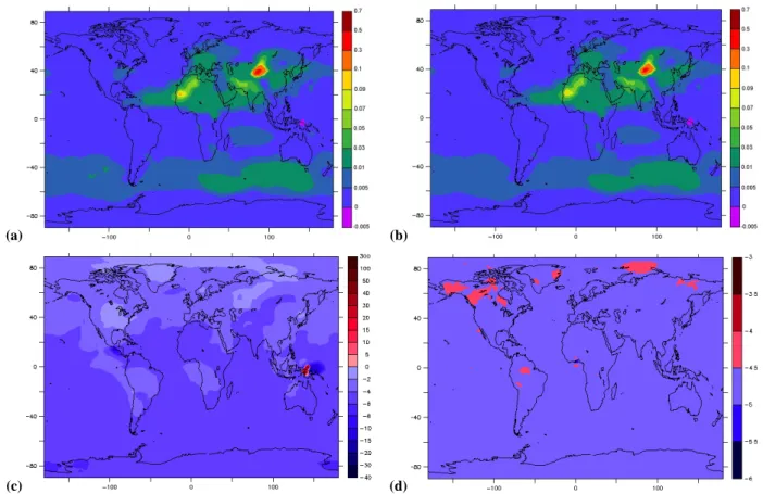
The simplified model simulates the main features of the horizontal distribution of the burden of gaseous precursors (species 1) (Fig. 1). The model reproduces the maxima over the continents, underestimates the burden in the southern hemisphere and Equatorial Pacific and overestimates it over the Atlantic Ocean in the northern hemisphere. The main rea-son for these differences is the simplification of the sulphur chemistry. In the original model the sulphur chemistry is limited by the availability of oxidants as O3, H2O2, OH and NO3 radicals. In SPLA however, the chemistry of sulphur depends on a chemical lifetime that varies only with respect to latitude. The differences in Fig. 1 between both models coincide with the variability of these oxidants (not shown). The overestimation is produced in the regions where there is a larger oxidant concentration due to a larger influence of anthropogenic emissions whereas the underestimation is produced in regions with cleaner air and thus with a smaller oxidant concentration. The parameterization of the chemical lifetime in the sulphur chemistry in SPLA does not differen-tiate between hemispheres according to the concentration of oxidants for two points at the same latitude. This can pro-duce the overestimate of SO2, (species 1) in regions with a higher concentration of oxidants through a smaller conver-sion of SO2in sulphate and an underestimate of SO2in re-mote regions with cleaner air through a larger conversion.

Another reason for the differences above the ocean of the southern hemisphere is the difference in deposition velocities between the two models. The regions with an underestima-tion of the burden correspond to regions where DMS dom-inates with respect to other species considered in species 1. The deposition velocity for DMS increased from 0.0 cm s−1 in LMDz (Table 1) to 2.8 cm s−1in SPLA (Table 3), hence

(7)

Fig. 1. Sulphur burden [mg S/m2] of sulphur gases (i.e. SO2, DMS, H2S) considered in species 1 according to LMDz (left) and to SPLA (right). Both burdens represent the yearly average of the year 2000.

the simplified model now presents dry deposition where be-fore there was no dry deposition. However, this explana-tion is not valid in the Northern Hemisphere oceans where an overestimation is observed. In these regions the over-estimation is more likely linked to the SO2 concentration than to DMS. The SO2presents a deposition velocity smaller in SPLA than in LMDZ (Tables 3 and 1, respectively) and produces therefore the opposite effect than observed over oceanic regions in the southern hemisphere and Equatorial pacific.

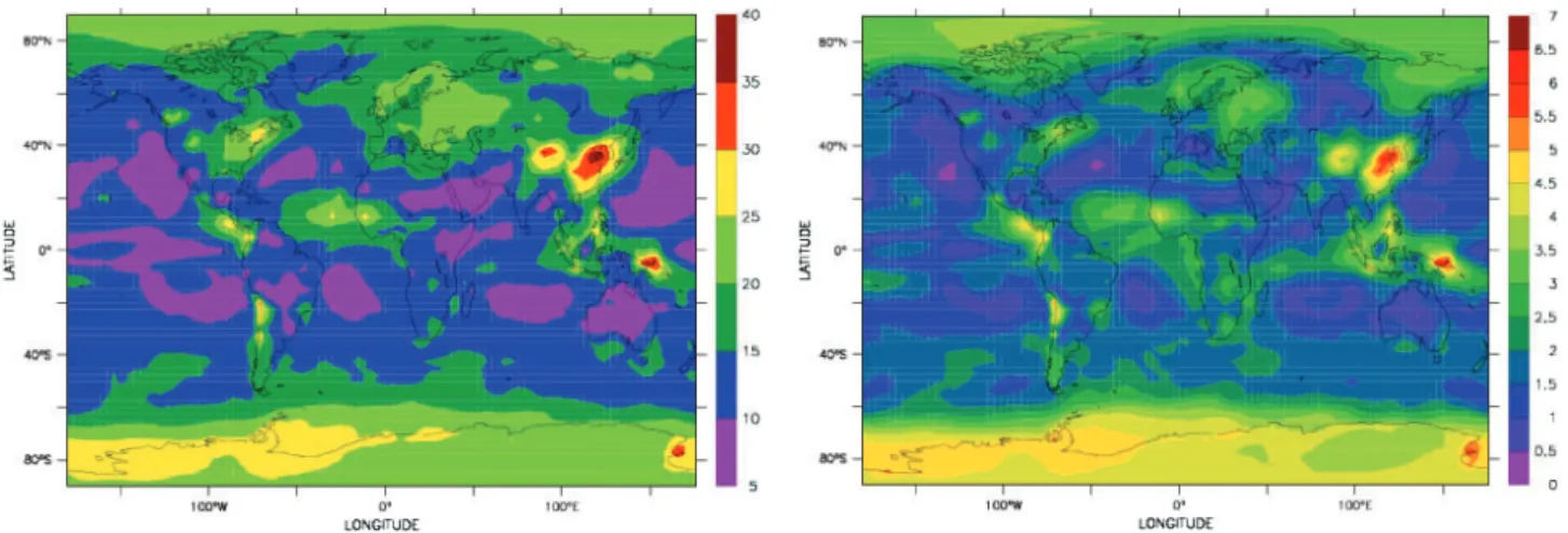
SPLA reproduces the horizontal distribution of species 2 with maxima over Africa, Middle East, Central Asia and Southeast Asia presenting only minor differences with re-spect to LMDz (Fig. 2). However, it overestimates the bur-den over Eastern Asia and Eastern Europe. The maximum in burden over North and Central Africa is associated to desert dust and biomass burning and the corresponding differences between both models is due to the increase in the tion velocity in SPLA (Table 3) increasing thus the deposi-tion flux and decreasing the burden of species 2 with respect to LMDz. Despite the important contribution of BC, OM and DD to species 2 over Eastern Asia, the overestimation in bur-den is produced by the decrease of the sulphate deposition velocity in SPLA. This last also explains the overestimate observed over the oceans.

The coarse mode of DD (species 3) is equivalent to the coarse mode of DD in the original model and thus presents the smallest differences (Fig. 3). Finally, for SS (species 4), the difference between both models are due to the different mass median diameters used in computing the sedimentation (Fig. 4).

Aerosol optical depth at 550 nm

The AOD of both models is now compared at 550 nm in terms of the root mean square error (RMSE) of the simpli-fied model with respect to LMDz. The RMSE of the daily

and monthly averages is presented in Fig. 5. A much higher difference is observed in the RMSE of the daily average than the monthly one. The differences in the daily variability can go up to 40%, whereas the difference in monthly variability does not exceed 7%, indicating a larger difficulty of SPLA to simulate the daily variability than the monthly one. The largest differences between both models are observed over Southeast Asia and north of Australia. These differences are mainly due to the differences in the burden observed for species 1 and 2 and described in the previous section.

3.2.2 Comparison of SPLA against AERONET measurements

We compare the AOD at 550 nm from SPLA against AERONET measurements. This is a global network of pho-tometers that delivers numerical data to monitor and char-acterize the aerosols in a regional and/or global scale. The network has more than 300 stations distributed in the world measuring clean atmosphere in remote regions and polluted areas (Holben et al., 1998). For the present analysis we use SPLA and LMDz simulations for the year 2000 and coinci-dent AERONET data.

A set of AERONET sites have been chosen to evaluate the performance of SPLA with respect to the different types of aerosol simulated. These sites represent the influence of fos-sil fuel combustion, biomass burning, desert dust and sea salt. We compare the monthly and daily data of AOD at 550 nm for the year 2000. Only days with AERONET measurements are considered when computing the model monthly average. LMDz is also included in the analysis. A more exhaus-tive validation of LMDz against AERONET measurements is given in Reddy et al. (2005).

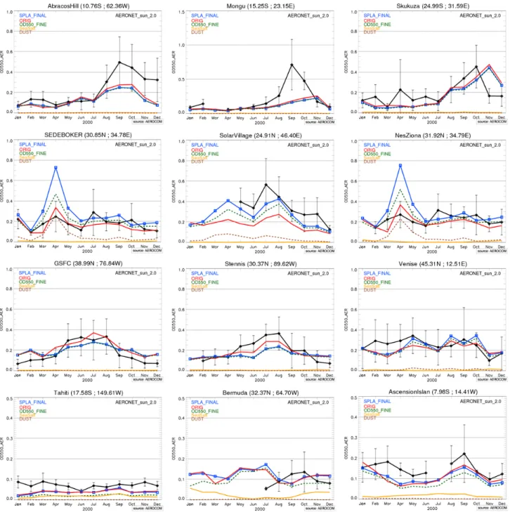
The measurements in the first group of sites (Abracos Hill, Mongu and Skukuza), are mainly influenced by biomass burning and present an annual cycle with maximal values of AOD towards the end of the year (Fig. 6). SPLA follows

(8)

Fig. 2. Same as Fig. 1 but for aerosols in species 2, i.e. SU, OM, BC, DD with radius between 0.03 and 0.5 µm and SS with radius smaller

than 0.5 µm. Units are in mg S/m2.

Fig. 3. Same as Fig. 1 but for DD aerosols with radius between 0.5 and 10 µm (species 3). Units are mg DD/m2.

(9)

Fig. 5. Normalized root mean square error (RMSE) of the total aerosol optical depth at 550 nm for daily (left) and monthly (right) averages

of SPLA with respect to LMDz.

closely the monthly variability of LMDz and its AOD is fully determined by species 2. It slightly underestimates LMDz during the month of maximum AOD which can be attributed to the increase in deposition velocity of species 2 (Table 3 and 1). Both models reproduce the seasonal cycle of biomass burning with larger differences in the biomass burning season and a shift of 1 or 2 month in the peak of AOD. The differ-ence between models and measurements is associated to a possible underestimation of emission sources (Reddy et al., 2005).

The simplified model reproduces the seasonal variabil-ity of both LMDz and AERONET at stations dominated by desert dust (Sede Boker, Solar Village and Nes Ziona) (Fig. 6). The model overestimates the AOD of LMDz throughout the year especially during the seasonal maxima of April in Sede Boker and Nes Ziona and April/August in So-lar Village. This is caused by an underestimation of the sed-imentation, caused partly by the absence of sedimentation of the fine mode DD in SPLA. The overestimation of AOD by SPLA improves its performance with respect to AERONET at Solar Village. The simplified model stays within the range of the observations during most of the year at all stations. The total AOD of SPLA is attributed to species 2 and 3 (DD). The sites mainly affected by industrial aerosols (GSFC, Stennis and Venice) present an annual cycle with maximal values of AOD during the summer month in the north Amer-ican sites of GSFC and Stennis whereas Venice presents rela-tively constant measurement around 0.2 throughout the year (Fig. 6). SPLA shows different performance for these two distinct types of sites. It underestimates the measurements in the month of maximum AOD for the North American sites whereas it overestimates it at Venice in the second half of the year. For the former the underestimation is probably due to the simplification in conversion of SO2to sulphate which does not take into account the increase of oxidation rate in summer while in Venice the overestimation is due to episodic dust transport from Africa.

Finally, the stations of Tahiti, Bermuda and Ascension Island, influenced by marine aerosols (i.e. sea salt and natural sulphur) and long range transport of continental aerosols (Reddy et al., 2005), present relatively constant cy-cle throughout the year with small amplitude peaking in dif-ferent times of the year according to the station (Fig. 6). Both models predict the seasonal cycle in agreement with the mea-surement with magnitudes within the range of the AOD. The three stations are affected by different sources and aerosol types; Tahiti is dominated by sea salt and sulphate, Bermuda is by marine aerosols in addition to dust from Africa and sul-phate from North America and finally Ascencion Island is influenced by sea salt in addition to carbonaceous aerosols from Africa (Reddy et al., 2005).

The simplified model follows closely and with negligible differences the AOD from LMDz throughout the year at all stations. The differences between models can be explained by changes in deposition velocities, sedimentation and the simplification of the sulphur chemistry as well as the modifi-cations introduced in the computation of the AOD.

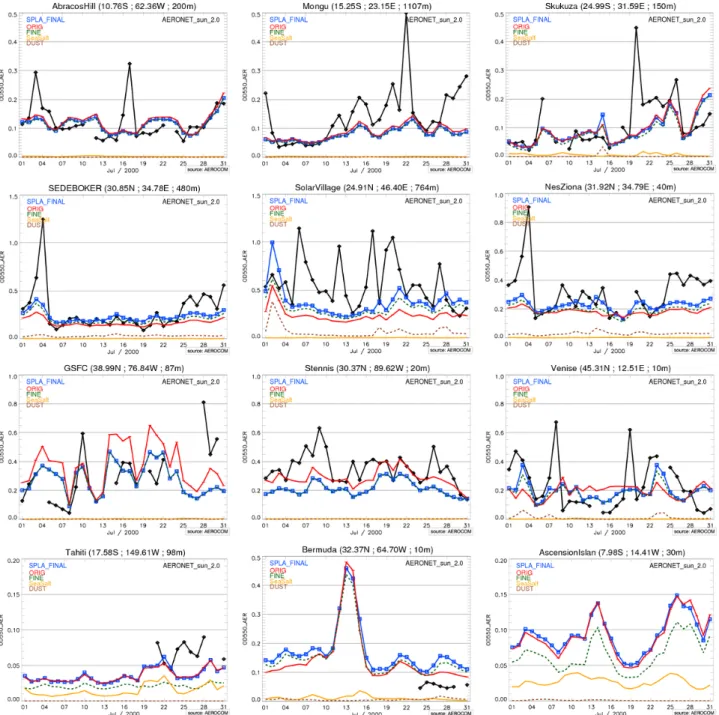
The model performance to simulate the daily variability is analyzed by reproducing the above analysis but with daily data. For practical reasons we limit the analysis to the month of July 2000 (Fig. 7).

Compared to the seasonal variability, SPLA has more dif-ficulties in reproducing the AERONET daily variability. The model reproduces the baseline AOD but does not always manage to reproduce the episodic increment of the aerosol load in most of the selected sites. The reduced number of measurement in sea salt stations does not allow to explore the performance for this aerosol specie. The simplified model however, follows closely the original model at all stations throughout the month. The largest differences are observed in stations affected by industrial aerosols (GSFC, Stennis and Venice) (Fig. 7). The same reasons as for the monthly vari-ability apply to explain the differences.

(10)

Fig. 6. Monthly averages of optical thickness of LMDz (red line) and SPLA (blue line) for twelve AERONET stations. The monthly averages

of both models were calculated using the days of the year with available AERONET measurements. Mean monthly values of AERONET are given by black rectangles and the error bars correspondent to the standard deviation of daily means around the monthly value. The optical thicknesses from the individual species of the SPLA scheme are also included; fine mode (tracer 2) corresponds to the green discontinuous line, coarse desert dust (tracer 3) to the brown discontinuous line and coarse sea salt (tracer 4) to the yellow continuous line.

Similar performance was obtained when comparing the model AOD against LMDz and AERONET at 670 and 865 nm for the same sites (figures not shown).

4 Tangent linear and adjoint model 4.1 Tangent linear model

The tangent linear model corresponds to the linearized equa-tions at a given state of a non-linear model. It provides a first order approximation to the evolution of perturbations in the input parameters. For a given model H denoted by Eq. (1)

(11)

Fig. 7. Daily values of optical thickness of LMDz (red line) and SPLA (blue line) for twelve AERONET stations. Daily measurements of

AERONET are given by black rectangles. The optical thicknesses from the individual species of the SPLA scheme are also included; fine mode (tracer 2) corresponds to the green discontinuous line, coarse desert dust (tracer 3) to the brown discontinuous line and coarse sea salt (tracer 4) to the yellow continuous line.

the tangent linear model is then:

δy = Hδx (7)

with H the matrix of derivatives of H also known as the ja-cobian matrix. We follow here and elsewhere the notation of Ide et al. (1997). Each element of the Jacobian matrix is given by the partial derivatives of the output (fine mode and total AOD) with respect to the input (emission fluxes and the

chemical lifetime of gaseous precursors):

H(i,j ) = ∂τi

∂ej

(8)

where i corresponds to all output parameters and j to all in-put parameters. Each comin-putation with the tangent linear provides the sensitivities of all output parameters with re-spect to one input parameter, i.e. one column of the Jacobian matrix.

(12)

The tangent linear of SPLA was derived using an auto-matic differentiation tool called TAPENADE (Hasco¨et and Pascual, 2004; Hasco¨et, 2004), while use is made here of the tangent linear code of the LMDz transport modules (Chevallier et al., 2005). This tangent linear model version has been numerically validated with the Taylor formula.

The forward model as observation operator computes the AOD fields comparable to satellite products such as those delivered by MODIS (Remer et al., 2005) and PARASOL (Deuz´e et al., 2000; Deuz´e et al., 2001) and any other satellite AOD product within the model wavelength range.

4.1.1 Model linearity

A linear observation operator H implies a quadratic cost function which facilitates the minimization of the cost func-tion. In order to deal with non-linear models, the minimizer in the variational data assimilation system needs to handle quadratic cost functions. The minimization of these non-quadratic functions can be obtained with an increase of the computational load (e.g., higher number of iterations) com-pared to the linear case (e.g. Tr´emolet, 2004).

We first conduct two SPLA runs using in one case an un-perturbed state (H (x)) and in the other case a un-perturbed one (H (x+δx)) with δx the perturbation. We define as total ini-tial perturbation the difference between these two states. We then apply the initial perturbation to the tangent linear model and compare it with the difference between the two SPLA runs. The difference between the total initial perturbation (H (x)-H (x+δx)) and the tangent linear one (Hδx) provides the non-linear part of the perturbation that is not explained by the linearized model.

We apply a rather small perturbation (10%) to the aerosol emission fluxes and chemical lifetime of gaseous precur-sors. Both, the perturbed and unperturbed emission fluxes are within the range of emissions of global models analyzed in Textor et al. (2006). We explore the linearity for the month of July 2002 and analyze the corresponding pertur-bations in total AOD at 550 nm. The tangent linear model (Fig. 8b) shows similar perturbations than the difference be-tween the perturbed and unperturbed simulations (Fig. 8a). Both present the same horizontal distributions, namely max-imum sensitivity in AOD to perturbations in the emissions of desert dust particularly over Central Asia, large sensitivities to emissions of sea salt and of fine mode aerosols (species 2). The sensitivities to the emissions of fine mode aerosols occur over regions with industrial and fossil fuel emissions. The part of the non-linear model not explained by the linearized model is presented in Fig. 8c in percentage. The largest dif-ferences are now observed north of New Guinea (Fig. 8c) in a region of important gaseous precursor burden (Fig. 1). The pattern of the discrepancies for both, fine and total AOD, cor-responds to regions with large root mean squares for daily and monthly averages (Fig. 5). Sensitivity tests were con-ducted by repeating the above mentioned experiment while

excluding a different process each time. When sulphur chem-istry is turned-off (Fig. 8d) differences between Fig. 8a and b are strongly reduced indicating that the chemical produc-tion of SU (Eq. 2) is mostly responsible for the non-linearity of the model. A similar result with a smaller magnitude is observed when analyzing the discrepancies between tangent linear model and the total initial perturbation with respect to the fine mode AOD at 550 nm (not shown).

4.1.2 Model sensitivities

We focus our analysis in examining the perturbations in the total AOD. Results correspond to the month of July 2002. The Jacobian matrix, (or matrix of derivatives of AOD with respect to emissions) is computed with the tangent linear model.

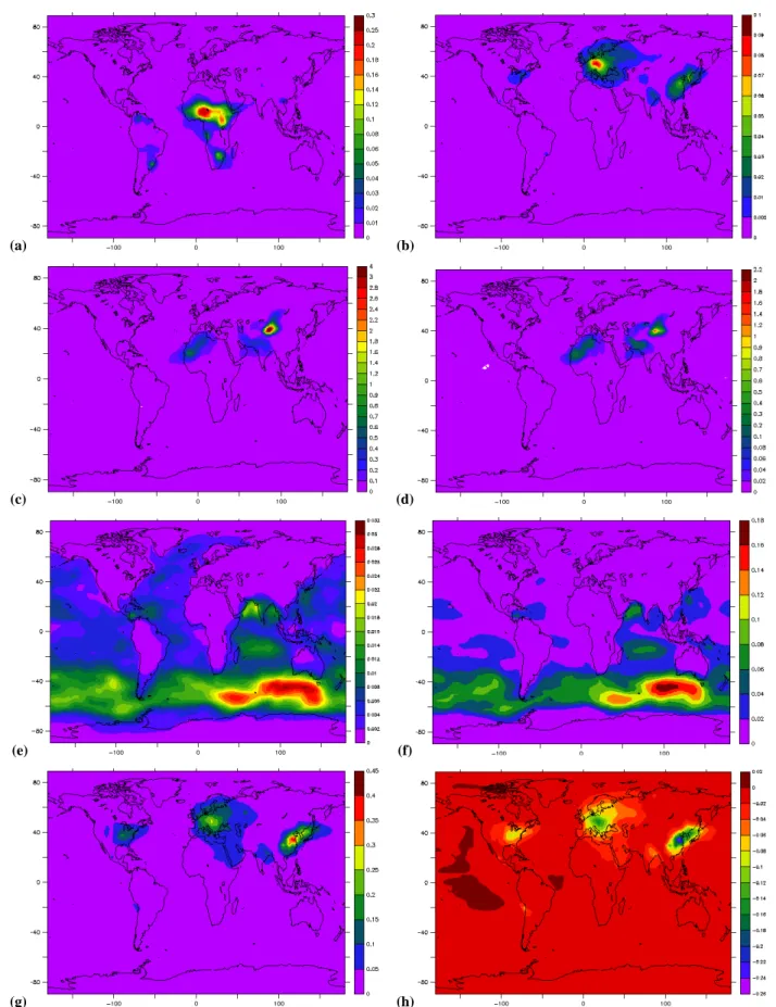
We simultaneously analyze the perturbations on AOD at 550 nm due to perturbations in the emissions of biomass burning (BB) and fossil fuel (FF) (Fig. 9a and b, respec-tively); both represent carbonaceous emission and thus will ease the comparison with the global cycle of carbona-ceous aerosols in LMDz (original model) as presented in Reddy and Boucher (2004). The total AOD at 550 nm presents positive sensitivities to the carbonaceous sources over Africa, Southeast Asia, Europe and South America co-incident with the AOD distribution presented in Reddy and Boucher (2004). This reflects that an increase in emissions translates into a regional increase of AOD consistent with what is expected. Largest sensitivities are seen over sub-Saharan Africa for BB (Fig. 9a) and Europe for FF (Fig. 9b) with the sensitivity to BB emissions being almost a factor three larger than that for FF. Smaller sensitivities are ob-served in South America, Central and South Africa for BB and Southeast Asia, India, South Africa and North and South America for FF emissions. Some differences are appreciable over South America and Southeast Asia.

Fine mode and coarse mode desert dust present the same horizontal distribution of sensitivities associated to the main dust load contributors (Prospero, 1996; Tanaka and Chiba, 2006); maxima over Central Asia and smaller sensitivities associated to the sources in the Middle East and the Saharan desert (Fig. 9c and d, respectively). However, differences in the intensity can be noted. The fine mode sensitivities are al-most twice those of the coarse mode. The previous is because in SPLA the fine mode has larger values of single scattering albedo than the coarse mode, i.e. the fine mode desert dust is more efficient in scattering light than the coarse mode. Thus for the same perturbation in emissions the fine mode will produce a larger perturbation in AOD than the coarse mode. The sensitivity distribution presented agrees with the hori-zontal distribution of desert dust AOD presented in Reddy et al. (2005). The same feature is observed when comparing to the AOD from different models presented in Tegen (2003).

The total AOD presents sensitivity to emissions of fine mode (Fig. 9e) and coarse mode (Fig. 9f) sea salt aerosols all

(13)

(a) (b)

(c) (d)

Fig. 8. Total AOD at 550 nm for July 2002 for (a) the difference between perturbed and unperturbed simulations of SPLA, (b) the tangent

linear of SPLA, (c) the difference of panels b) and a) expressed in percentage with respect to (a) and (d) the same as (c) but when sulphur chemistry is turned-off.

over the southern ocean with maximal sensitivities over the southern ocean (20◦E–150◦E). Lower latitude regions with local maximal sensitivity correspond to the Indian Ocean and the Arabian Sea. This distribution agrees well with the horizontal distribution of sea salt burden presented in Ma et al. (2008). However differences are observed when compar-ing to the AOD distribution in Reddy et al. (2005), especially in the northern ocean where no important sensitivity regions are observed corresponding to the regional maxima of sea salt AOD.

For the analysis of the model sensitivities with respect to SU emissions and its gaseous precursors, we perturb on one hand the emissions of gaseous precursors simultaneously with the SU emissions and on the other hand we also perturb the SU production from its gaseous precursors (described in Sect. 3.1). For the latter, a positive perturbation increases the lifetime of gaseous sulphur species and therefore reduces sulphate production for a same period of time. Consequently the AOD sensitivities to perturbations in the chemical life-time present negative values; a positive perturbation in the chemical lifetime decreases sulphate production, its atmo-spheric load and the AOD (Fig. 9h). The AOD sensitivities to perturbation in gaseous precursors and SU emissions on the contrary present positives values coherent with the fact that a

higher load of SU aerosols increases the AOD (Fig. 9g). Both sensitivities present similar horizontal distribution but with opposite sign and stronger sensitivity for SU emissions; the AOD at 550 nm is more sensitive to the emissions of gaseous precursors and SU than to chemical production of SU. The maxima (in absolute terms) are located over the continents in the Northern Hemisphere close to the emission sources. In both cases the largest maxima are located over Eastern Asia, followed by Europe, North America and Central Asia. A small region of sensitivity is observed in the Southern Hemi-sphere over western South America probably associated to copper smelters.

4.2 Adjoint model

The adjoint model provides the sensitivities of the input pa-rameters to perturbation in the output papa-rameters. For a for-ward model H and its tangent linear model H, the adjoint model is

x∗=HTy∗ (9)

where HT is the adjoint model and the transpose of the Jacobian matrix H (Eq. 7), x∗ is the output sensitivities in the input space and y∗the input sensitivities in the observa-tion space.

(14)

(a) (b)

(c) (d)

(e) (f)

(g) (h)

Fig. 9. Sensitivities in the total AOD at 550 nm for the month of July 2002 to perturbations in emissions of: (a) biomass burning, (b)

fossil fuel, (c) fine mode desert dust, (d) coarse mode desert dust, (e) fine mode sea salt, (f) coarse mode sea salt, (g) gaseous and sulphate emissions and (h) gas-to-particle conversion. Units for figure (a) to (g) are [AOD/emission flux] whereas for (h) it is [AOD/conversion rate].

(15)

(a) (b)

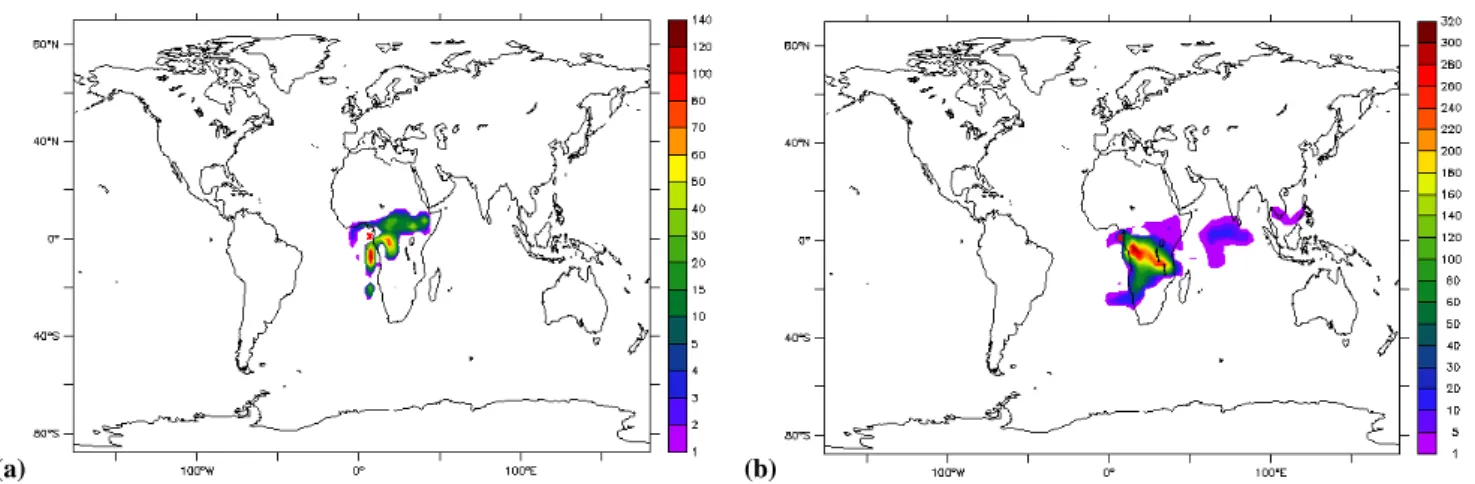
Fig. 10. Sensitivities of fine mode AOD at 550 nm off the coast of Central Africa to emissions of fine mode aerosols for a two day (a) and

five day long simulation (b). The exact location of the observation is indicated by a red cross.

As for the tangent linear model, the adjoint model of SPLA was derived using the automatic differentiation tool called TAPENADE and the adjoint code of the LMDz transport modules (Chevallier et al., 2005) was used. The adjoint model was found accurate to within 130 times the zero of the computer and the computational cost of the adjoint model is between 5 to 6 times that of the forward model. The accuracy of the test reveals the efficiency of the adjoint in the assimila-tion; the higher the accuracy the more efficient the variational minimization will be.

We use the adjoint model to present the sensitivities of the AOD to aerosol emissions. In contrast to the tangent linear model that computes the sensitivity in the AOD for perturba-tions in the emission field, the adjoint model allows to com-pute the perturbation in the emission field needed to produce a given signal in the AOD. To illustrate the adjoint sensitivi-ties we conceive an experiment where the y∗vector in Eq. (9) consists of a point and instantaneous perturbation in the fine mode AOD at 550 nm. This point perturbation is defined off the coast of central Africa for the last day of July 2002. Re-sults indicate the emission flux that is needed back in time to generate the given perturbation in AOD. All resulting sensi-tivities will relate to this particular observation.

We show the sensitivity in the emission field two and five days before the observation. The results correspond-ing to two days before identify the regions where emitted aerosol would create the given perturbation two days later. The fine mode AOD in that particular location is more sen-sitive to emissions of fine mode sea salt originated to the south than to biomass burning emissions from Central Africa (Fig. 10a). The wind field for the simulated days presents predominant southerly winds in the lower layers of the at-mosphere and easterly winds increasing in magnitude with increasing height (not shown). Five days prior the obser-vation however the highest sensitivity is now observed over sub-Saharan Africa and only weak sensitivities are observed

in distant ocean regions (Fig. 10b). The maximum sensi-tivities over Africa coincide with the southeasterly winds whereas the long range transport from south of the Indian subcontinent is due to the large scale easterly winds at higher levels (not shown).

5 Conclusions

Uncertainties in aerosol emissions introduce uncertainties about their final impact on climate. Previous works have used variational data assimilation techniques to estimate the emis-sion field for single aerosol species. This field represents the best compromise between a given set of observations and the a priori information. This work however, presents a first step towards estimating the intensity of the emissions of a range of aerosol species through variational data assimila-tion. For this purpose the general circulation model LMDz in its version 3.3 has been simplified into the Simplified Aerosol Model (SPLA) and its corresponding tangent linear and ad-joint versions were derived.

The complexity of LMDz for the simulation of the global life cycle for the main aerosol species (SS, DD, OM, BC and SU) was reduced in SPLA. This model groups together the 24 aerosol species simulated in LMDz into 4 species, namely the gaseous precursors, the fine mode aerosols, the coarse mode of desert dust and the coarse mode of sea salt. As a consequence of this, several modifications had to be in-troduced; the deposition velocity of each new species was adapted according to the species it contained, the mass me-dian diameter for the sedimentation of only coarse mode aerosol, both SS and DD, was also adapted to represent their new size distribution and the mass extinction efficiencies were recomputed according to the new species. Furthermore, the sulphur chemistry was reduced to an oxidation mecha-nism as a function of latitude and no distinction between hy-drophilic and hydrophobic OM and BC was done.

(16)

The performance of SPLA was evaluated by comparing it against LMDz in terms of burden and AOD and against AERONET AOD. The simplified model successfully man-ages to reproduce the main features in LMDz of the horizon-tal distribution of the burden for each one of the species. The main differences between the models are on one hand due to differences in the deposition and sedimentation fluxes associ-ated to new deposition and sedimentation velocities, respec-tively and on the other hand to the simplification of the sul-phur chemistry to a simple oxidation of sulsul-phur to sulphate. Distinct behavior can be identified in the performance of the aerosol burden and the AOD. The largest differences with re-spect to the burden are observed in species 1 and 2 where most of the modifications were introduced, while species 3 and 4 keep more similarities with their original counterpart and therefore do not differ greatly. The largest differences in AOD, with both LMDz and AERONET, are observed over sites with strong DD influence (species 3). However, sim-ulated AOD remains within the variability of the observa-tions for all species and all sites throughout most of the year. SPLA follows closely the seasonal cycle of LMDz and has therefore a similar performance to LMDz in simulating total AOD. Finally, the model has a better performance in repro-ducing the monthly variability of LMDz than in reproduc-ing the daily one. SPLA reproduces the baseline AOD of the AERONET daily data but has difficulties in reproducing the daily variability associated to episodic increment in the aerosol load. The largest differences are observed in stations affected by industrial aerosols. However, it closely repro-duces the LMDz daily variability at all stations throughout the month.

The simplified model shows some differences in the sen-sitivities between the tangent linear model and the SPLA when perturbing the emission fluxes and chemical lifetime rate by 10%. These differences illustrate the non-linearity of the simplified model, which is mostly due to the simpli-fied sulphur chemistry. When examining in more detail the sensitivities of SPLA, the model shows positive sensitivities for perturbations in the emission flux but negative ones when perturbing the chemical lifetime of gaseous precursors. This is consistent with the fact that a higher aerosol load increases the AOD whereas a positive perturbation in the chemical life-time rate increases the duration of gaseous sulphur species and thus reduces sulphate production and AOD with it. Max-imum sensitivities for each aerosol species coincide with re-gions of maximal AOD situated over and in the vicinity of emission regions coherent with the known regional impact of aerosols. The sensitivity analysis reveals differences with respect to the original model in the location of BB sources over South America.

The tangent linear and the adjoint models of SPLA have been derived through automatic differentiation and were found numerically accurate. They were implemented together with the direct model described in this work in the variational data assimilation scheme of Chevallier et

al. (2005). Daily averages of total and fine mode AOD from MODIS at 550 nm will be assimilated and the estimation of the intensity of the emissions for the five main aerosol species (SU, BC, OM, DD and SS) will be derived. The re-sults of this work will be presented in a forthcoming publica-tion.

Acknowledgements. Olivier Boucher was supported by the Joint DECC, Defra and MoD Integrated Climate Programme – (DECC) GA01101, (MoD) CBC/2B/0417 Annex C5. The authors would like to thank the AERONET program for establishing and maintain-ing the used sites. Furthermore, we thank the AEROCOM model team for making available the model-AERONET comparison software and facilitate the comparison of SPLA with LMDz and AERONET. We acknowledged the reviewers for providing useful comments that helped to improve the manuscript. This study was co-funded by the European Commission under the EU Seventh Research Framework Programme (grant agreement No 218793, MACC). TAPENADE can be downloaded from http://www-sop.inria.fr/tropics/tapenade.html.

Edited by: A. Sandu

The publication of this article is financed by CNRS-INSU.

References

Benedetti, A., Morcrette, J.-J., Boucher, O., Dethof, A., Engelen, R. J., Fisher, M., Flentjes, H., Huneeus, N., Jones, L., Kaiser, J. W., Kinne, S., Mangold, A., Razinger, M., Simmons, A. J., and Suttie, M.: Aerosol analysis and forecast in the European Centre for Medium-Range Weather Forecasts Integrated Forecast System: 2: Data assimilation, J. Geophys. Res., 114, D13205, doi:10.1029/2008JD011115, 2009.

Boucher, O. and Pham, M.: History of sulphate aerosol radiative forcings, Geophys. Res. Lett., 29(9), 1308, doi:10.1029/2001GL014048, 2002.

Boucher, O., Pham, M., and Venkataram, C.: Simulation of the at-mospheric sulphur cycle in the Laboratoire de M´et´eorologie Dy-namique general circulation model: Model description, model evaluation, and global and european budgets, Note Sci. IPSL 23, 27 pp., Inst. Pierre Simon Laplace, Paris, available at http://www. ipsl.jussieu.fr/poles/Modelisation/NotesSciences.htm, 2002. Chevallier, F., Fisher, M., Peylin, P., Serrar, S., Bousquet, P.,

Br´eon, F.-M., Ch´edin, A., and Ciais, P.: Inferring CO2 sources and sink from satellite observations: Methods and application to TOVS data, J. Geophys. Res., 110, D24309, doi:10.1029/2005JD006390, 2005.

Chevallier, F., Fortems, A., Bousquet, P., Pison, I., Szopa, S., De-vaux, M., and Hauglustaine, D. A.: African CO emissions be-tween years 2000 and 2006 as estimated from MOPITT

(17)

observa-tions, Biogeosciences, 6, 103–111, 2009, http://www.biogeosciences.net/6/103/2009/.

Cooke, W. F. and Wilson, J. J. N.: A global black carbon aerosol model, J. Geophys. Res., 101, 19395–19409, 1996.

Cooke, W. F., C., Liousse, H., Cachier, and J. Feichter, : Con-struction of a 1◦×1◦fossil fuel emission data set for carbona-ceous aerosol and implementation and radiative impact in the ECHAM4 model, J. Geophys. Res., 104, 22137–22162, 1999. Deuz´e, J.-L., Goloub, P., Herman, M., Marchand, A., Perry, G.,

Tanr´e, D., and Susana, S.: Estimate of the aerosols properties over the ocean with POLDER, J. Geophys. Res., 105, 15329– 15346, 2000.

Deuzé, J.-L., Bréon, F.-M., Devaux, C., Goloub, P., Herman, M., Lafrance, B., Maignan, F., Marchand, A., Nadaf, L., Perry, G., and Tanré, D.: Remote sensing of aerosols over land surfaces from POLDER-ADEOS 1 Polarized measurements, J. Geophys. Res., 106, 4913–4926, 2001.

Dubovik, O., Lapyonok, T., Kaufman, Y. J., Chin, M., Ginoux, P., Kahn, R. A., and Sinyuk, A.: Retrieving global aerosol sources from satellites using inverse modeling, Atmos. Chem. Phys., 8, 209–250, 2008,

http://www.atmos-chem-phys.net/8/209/2008/.

Elbern, H., Strunk, A., Schmidt, H., and Talagrand, O.: Emission rate and chemical state estimation by 4-dimensional variational inversion, Atmos. Chem. Phys., 7, 3749–3769, 2007,

Forster, P., Ramaswamy, V., Artaxo, P., Bernsten, T., Betts, R., Fa-hey, D. W., Haywood, J., Lean, J., Lowe, D. C., Myhre, G., Nganga, J., Prinn, R., Raga, G., Schulz, M., and van Dorland, R.: Changes in Atmmospheric Constituents and in Radiative Forc-ing, in: Climate Change 2007: The Physical Science Basis. Con-tribution of Working Group I to the Fourth Assessment Report of the Intergovenmental Panel on Climate Change, edited by: Solomon, S., Qin, D., Manning, M., Chen, Z., Marquis, M., Av-eryt, K. B., Tignor, M., and Miller, H. L., Cambridge University Press, Cambridge, UK, and New York, NY, USA, 2007. Guelle, W., Balkanski, Y. J., Schulz, M., Marticorena, B.,

Berga-metti, H., Moulin, C., Arimoto, R., and Perry, K. D.: Model-ing the atmospheric distribution of mineral aerosol: Compar-isons with ground measurements and satellite observations for yearly and synoptic timescales over the North Atlantic, J. Geo-phys. Res., 105, 1997–2012, 2000.

Hakami, A., D. K., Henze, J. H., Seinfeld, T., Chai, Y., Tang, G. R., Carmichael, and A. Sandu, : Adjoint inverse mod-eling of black carbon during Asian Pacific Regional Aerosol Characterization experiment, J. Geophys. Res., 110, D14301, doi:10.1029/2004JD005671, 2005.

Hasco¨et, L. and Pascual, V.: TAPENADE 2.1 user’s guide, Rapport Technique Nr. 3000, Institut National de Recherche en Informa-tique et en AutomaInforma-tique (INRIA), 78 pp., 2004.

Hasco¨et, L.: TAPENADE: A tool for automatic differentiation for programs, European congress on computational methods in ap-plied sciences and engineering, ECCOMAS, 14 pp., 2004. Henze, D. K., Seinfeld, J. H., Liao, W., Sandu, A., and

Carmichael, G. R.: Inverse modelling of aerosol dynamics: Condensation growth, J. Geophys. Res.-Atmos., 109, D14201, doi:10.1029/2004JD004593, 2004.

Henze, D. K., Seinfeld, J. H., and Shindell, D. T.: Inverse model-ing and mappmodel-ing US air quality influences of inorganic PM2.5

precursor emissions using the adjoint of GEOS-Chem, Atmos. Chem. Phys., 9, 5877–5903, 2009,

Holben, B. N., Eck, T. F., Slutsker, I., Tanr´e, D., Buis, J.-P., Set-zer, A., Vermote, E., Reagan, J. A., Kaufman, Y. J., Nakajima, T., Lavenu, F., Jankowiak, I., and Smirnov, A.: AERONET – A federated instrument network and data archive for aerosol char-acterization, Remote Sens. Environ., 66, 1–13, 1998.

Ide, K., Courtier, P., Ghil, M., and Lorenc, A. C.: Unified notation for data assimilation : Operational, sequential and variational, J. Meteorol. Soc. Jpn., 75(1B), 181–189, 1997.

Kopacz, M., Jacob, D. J., Henze, D. K., Heald, C. L., Streets, D. G., and Zhang, Q.: A comparison of analytical and adjoint Bayesian inversion methods for constraining Asian sources of CO using satellite (MOPITT) measurements of CO columns, J. Geophys. Res., 114, D04305, doi:0.1029/2007JD009264, 2009.

Ma, X., von Salzen, K., and Li, J.: Modelling sea salt aerosol and its direct and indirect effects on climate, Atmos. Chem. Phys., 8, 1311–1327, 2008,

Meirink, J. F., Bergamaschi, P., Frankenberg, C., et al.: Four-dimensional variational data assimilation for inverse mod-elling of atmospheric methane emissions: Analysis of SCIA-MACHY observations, J. Geophys. Res., 113, D17301, doi:10.1029/2007JD009740, 2008.

Monahan, E. C., Spliel, D. E., and Davidson, K. L.: A models of marine aerosol generation via whitecaps and wave disruption, in oceanic whitecaps, edited by: Monahan, E. C. and Mac Niocail, G., Springer, New York, 167–174, 1986.

Morcrette, J.-J., Boucher, O., Jones, L., Salmond, D., Bechtold, P., Beljaars, A., Benedetti, A., Bonet, A., Kaiser, J. W., Razinger, M., Schulz, M., Serrar, S. Simmons, A. J., Sofiev, M., Suttie, M., Tompkins, A. M., and Untch, A.: Aerosol analysis and forecast in the ECMWF Integrated Forecast System: Forward modelling, J. Geophys. Res., 114, D06206, doi:10.1029/2008JD011235, 2009.

Olivier, J. G. J. and Berdowski, J. J. M.: Global emissions sources and sinks, in: The Climate System , edited by: Berdowski, J., Guicherit, R., and Heij, B. J., A.A. Balkerna, Brookfield, Vt, 33– 78, 2001.

Prospero, J. M.: The atmospheric transport of particles to the ocean, in: Particle Flux in the Ocean, edited by: Ittekott, V., Schaeffer, P., Honjo, S., and Depetris, P. J., Wiley, New York, 1996. Reddy, M. S. and Boucher, O.: A study of the global cycle of

car-bonaceous aerosols in the LMDZT general circulation model, J. Geophys. Res., 109, D14202, doi:10.1029/2003JD004048, 2004. Reddy, M. S., Boucher, O., Bellouin, N., Schulz, M., Balka-nski, Y., Dufresne, J.-L., and Pham, M.: Estimates of global multicomponent aerosol optical depth and direct radia-tive perturbation in the Laboratoire de M´et´eorologie Dynamique general circulation model, J. Geophys. Res., 110, D10216, doi:10.1029/2004JD004757, 2005.

Remer, L. A., Kaufman, Y. J., Tanr´e, D., Mattoo, S., Chu, D. A., Martins, J. V., Li, R.-R., Ichoku, C., Levy, R. C., Kleidman, R. G., Eck, T. F., Vermote, E., and Holben, B. N.: The MODIS aerosol algorithm, products and validation, J. Atmos. Sci., 62, 947–973, 2005.

Robertson, L. and Langner, J.: Source function estimate by means of variational data assimilation applied to the ETEX-I tracer

(18)

ex-periment, Atmos. Environ., 32, 4219–4225, 1998.

Sandu, A., Liao, W., Carmichael, G. R., Henze, D. K., and Sein-feld, J. H.: Inverse modeling of aerosol dynamics using adjoints: theoretical and numerical considerations, Aerosol Sci. Tech., 39, 677–694, 2005.

Schulz, M., Balkanski, Y., Dulac, F., and Guelle, W.: Role of aerosol size distribution and source location in a three-dimensional simulation of a Saharan dust episode tested against satellite-derived optical thickness, J. Geophys. Res., 103, 10579– 10592, 1998.

Stavrakou, T. and M¨uller, J.-F.: Grid-based versus big region ap-proach for inverting CO emissions using Measurement of Pollu-tion in the Troposphere (MOPITT) data, J. Geophys. Res., 111, D15304, doi:10.1029/2005JD006896, 2006.

Tanaka, T. Y. and Chiba, M.: A numerical Study of the contribu-tions of dust source regions to the global budget, Global Planet. Change, 52, 88–104, 2006.

Tegen, I.: Modeling the mineral dust aerosol cycle in the climate system, Quaternary Sci. Rev., 22, 1821–1834, 2003.

Textor, C., Schulz, M., Guilbert, S., et al.: Analysis and quantifi-cation of the diversities of aerosol life cycles within AeroCom, Atmos. Chem. Phys., 6, 1777–1813, 2006,

Tr´emolet, Y.: Diagnostics of linear and incremental approximation in 4D-Var, Q. J. Roy. Meteor. Soc., 130, 2233–2251, 2004. Yumimoto, K., Uno, I., Sugimoto, N., Shimizu, A., and

Sa-take, S.: Adjoint inverse modeling of dust emission and transport over East Asia, Geophys. Res. Lett., 34, L08806, doi:10.1029/2006GL028551, 2007.

Yumimoto, K., Uno, I., Sugimoto, N., Shimizu, A., Liu, Z., and Winker, D. M.: Adjoint inversion modeling of Asian dust emis-sion using lidar observations, Atmos. Chem. Phys., 8, 2869– 2884, 2008,

Zhang, J., Reid, J. S., Westphal, D. L., Baker, N. L., and Hyer, E. J.: A system for operational aerosol optical depth data as-similation over global oceans, J. Geophys. Res., 113, D10208, doi:10.1029/2007JD009065, 2008.