HAL Id: cea-01655036
https://hal-cea.archives-ouvertes.fr/cea-01655036
Submitted on 12 Jan 2018
HAL is a multi-disciplinary open access
archive for the deposit and dissemination of
sci-entific research documents, whether they are
pub-lished or not. The documents may come from
teaching and research institutions in France or
abroad, or from public or private research centers.
L’archive ouverte pluridisciplinaire HAL, est
destinée au dépôt et à la diffusion de documents
scientifiques de niveau recherche, publiés ou non,
émanant des établissements d’enseignement et de
recherche français ou étrangers, des laboratoires
publics ou privés.
Superconducting coils quench simulation, the Wilson’s
method revisited
Vincent Picaud, P. Hiebel, J.-M. Kauffmann
To cite this version:
Vincent Picaud, P. Hiebel, J.-M. Kauffmann. Superconducting coils quench simulation, the Wilson’s
method revisited. IEEE Transactions on Magnetics, Institute of Electrical and Electronics Engineers,
2002, 38 (2), pp.1253 - 1256. �10.1109/20.996320�. �cea-01655036�
Superconducting Coils Quench Simulation, the
Wilson’s Method Revisited
Vincent Picaud, Patrick Hiebel, and Jean-Marie Kauffmann
Abstract—This paper describes a new numerical method which
analyzes adiabatic quench of superconducting coils. The method is a generalization of the Wilson’s older method. With this new method the resistive front is not restricted to be an ellipsoid and can evolve with an arbitrary velocity at its border. The evolution of the resistive front is efficiently controlled by the introduction of the level-set method. The two-dimensional version presented here leads to a fast simulation code of the quench process.
Index Terms—Level-set method, quench, superconducting
magnet, superconductor.
I. INTRODUCTION
T
HE PREDICTION of the behavior of a superconducting coil during a transition from the superconducting state to the normal state is important because this phenomenon can lead to the destruction of the device. Historically the Wilson’s QUENCH [1] program was the first published code allowing quench simulation of a superconducting coil on a computer. Despite its simplicity, this approach gives globally correct results [3]–[5]. Another approach is to treat the coil as a anisotropic solid and solve the nonlinear heat equation gov-erning the quench process with methods like the finite-element method. But due to the existence of very strong temperature gradients such simulation required a large computing effort [2] (they use a Cray). We propose here an intermediate method which is more powerful than the Wilson’s method but which is still very fast compared with finite-element method oriented approaches. This method can be very interesting during the design process where a lots of configurations have to be tested with a moderate accuracy.II. THEWILSON’SMETHODREVISITED
A. The Wilson’s Method
The basic idea of the Wilson’s method is to introduce a front separating the resistive part from the superconducting part of the winding. This resistive front is an ellipsoid that grows with speed in the conductor direction and with speed
between the layers. The speed is the adiabatic propaga-tion speed for an isolated conductor, whereas the coefficient is the ratio of the propagation speed between layers of the winding
Manuscript received July 5, 2001; revised October 25, 2001.
V. Picaud is with the CreeBel Centre de recherche en Electronique et Electrotechnique de Belfort, and with the Laboratoire d’Electronique, Electrotechnique et Systemes, L2ES, 90000 Belfort, France (e-mail: [email protected]).
P. Hiebel and J.-M. Kauffman are with the Laboratoire d’Electronique, Elec-trotechnique et Systemes, L2ES, 90000 Belfort, France.
Publisher Item Identifier S 0018-9464(02)02770-X.
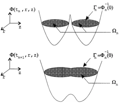
Fig. 1. Definition of and 0 using the level-set of a function 8. Evolution of : merging of two normal zones.
to the propagation speed along the conductor. The temperature rise in the normal zone is computed assuming local adiabaticity. This method has several drawbacks. It is difficult to control sev-eral fronts and to manage their intersections with the winding borders. Due to the imposed ellipsoidal shape of the normal zone the space variation of the speed cannot be taken into account.
B. Generalization
To generalize the Wilson’s method we consider an arbitrary resistive front evolving under an arbitrary velocity. Introducing the winding domain the normal zone can be modeled by a volume evolving under the action of a propagation speed imposed on its border . The normal zone cannot be connex (transition in several points of the winding) and change of topology in the course of time. The behavior of the resistive front is managed using the level-set method [8]. The principle of this method rests on the introduction of a function con-taining all the information on the resistive front. The normal zone and its border are defined by the level set of (Fig. 1). Introducing the cylindrical coordinates system we get
(1) (2) To find, in a formal way, the equation governing the evo-lution of we can use ideas from the method of characteris-tics. Assume that at time , the interface is parameterized by
1254 IEEE TRANSACTIONS ON MAGNETICS, VOL. 38, NO. 2, MARCH 2002
then the evolution of is determined by the equation
(3) Since is defined to be zero for all , we must have
(4) So, we get the classical convection equation which modelize the flow of in the velocity field . The previous calculus are rather formal and rigorous justifications of this approach can be found in [10]. Using the initial condition (8) it can be shown that (4) accurately moves the zero level set according to the velocity field even through the merging and breaking up of the volume
.
In our case, for a positive propagation speed, the front always expands. So the speed has to be chosen such that it is always in the direction of the gradient . This yields to the equation of motion of the normal zone
(5) Putting this in a more general framework the previous equa-tion is a Hamilton–Jacobi equaequa-tion
(6) where the Hamiltonian is:
(7) and the initial condition is:
(8) where
is the signed distance between
and negative if
Solutions of Hamilton–Jacobi equations can develop disconti-nuities in their derivatives. The numerical resolution of such equations requires the use of appropriate schemes in order to avoid spurious oscillations of the numerical solution [6], [7].
C. Space Discretization
We use a structured grid over the winding domain
and note and the forward and backward finite-differ-ence operators. The Hamiltonian (7) is not strictly convex so we use the classical nonconvex Lax–Friedrichs scheme. We use a second-order essentially nonoscillating (ENO) upwind ap-proximation of the derivatives [6], [7]. Assuming the speeds and stay positive we get the following simplified numerical scheme:
(9)
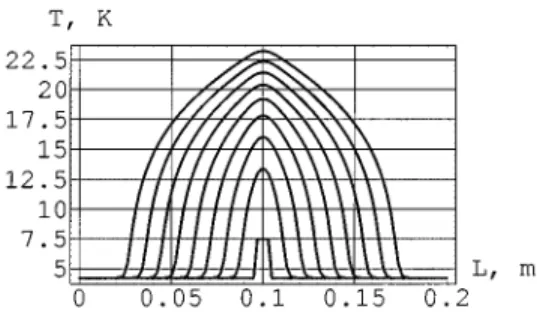
Fig. 2. Finite-element simulation of the conductor transition.
where and are the second-order ENO construction of the derivatives
(10) where denotes the ENO switch function
if
if if if
(11)
D. Time Discretization
In order to avoid oscillations of the solution the time numer-ical scheme must satisfied the total variation diminishing (TVD) property. We use a second-order TVD-Runge–Kutta scheme: the Heun method
(12) The previous scheme is stable if the Courant–Friedrich–Lewy condition (13) is satisfied. This condition with a security coeffi-cient is also used to dynamically adjust the time step during the simulation
(13)
III. PROPAGATIONSPEEDS
A. Longitudinal Propagation Speed
We use the classical one-dimensional quasilinear equation governing the temperature distribution in the conductor [14], [11], [13], [15]
(14) Starting from (14), several expressions for the normal zone propagation speed exist. In order to choose an analytical expres-sion we have developed a numerical simulation tool using the finite-element method (Fig. 2). In the light of the results, we use
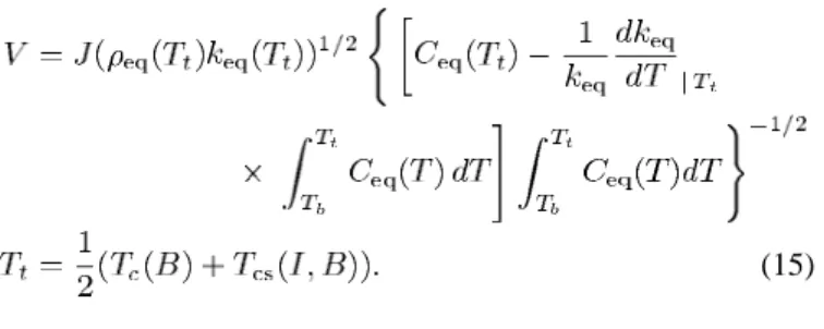
(15) [13] because it agrees very well with our numerical simu-lations.
(15)
B. Transverse Propagation Speed
To find the transverse propagation speed between the winding layers we introduce an elementary cell of the winding structure. This cell is constituted by conductors and epoxy resin. We note the ratio between the surface of conductors to the sur-face of the elementary cell
Following [12] we introduce a 1-D approximation of the winding structure constituted by two conductors of length separated by an epoxy layer of length . The calculation of the propagation speed between layers leads to the transverse propagation velocity
(16) IV. EVOLUTION OF THEOTHERQUANTITIES
The magnetic field and the inductance are evaluated using the Biot–Savart law. An analytical integration is performed for the and variables [17] while an adaptative Gauss–Kronrod integration rule [18] is used when analytical expressions are not accessible.
At time the total quench resistance of the coil is evaluated by numerical integration over the normal zone
(17) The temperature rise in the winding is evaluated assuming local adiabaticity. The resulting first order differential equation is integrated using the second-order Runge–Kutta scheme (12). (18) The electrical quantities are calculated using the same Runge–Kutta scheme. Like in the Wilson’s method we neglect the influence of the voltage drop induced by the mutual induction between the normal and the superconducting zone.
TABLE I
DESCRIPTION OF THETESTCOILS
(a) (b)
Fig. 3. Zero level set of8 showing the normal zone propagation in coil B (1t = 0:0075 s). (a) Quench starts at the bottom of the coil. (b) Quench starts at the middle of the inner radius.
Fig. 4. (Solid line) Quench starts at the bottom of the coil. (Dashed line) Quench starts at the middle of the inner radius.
For the case of a single coil transition we get (19) whereas for the transition of a coil protected by subdivision we get (20).
(19) (20) V. APPLICATIONS
We consider here the simulation of quench process in small NbTi coils. The dimensions of the structured rectangular grid used for each coil are and . Thus, the com-puting effort to solve (6) on this grid is very light. The coil B is initially energized with a current A, creating a mag-netic field of 3 T and a stored energy of 3207 J. To upgrade the magnetic field up to 4.3 T we add a second coil A. The coils A and B are protected by subdivision [11], [12]. (See Table I for a description of the test coils.)
1256 IEEE TRANSACTIONS ON MAGNETICS, VOL. 38, NO. 2, MARCH 2002
(a) (b)
Fig. 5. Protection by subdivision of the coils A and B.(a) Electrical circuit. (b) Quench process (I = 200 A, 1t = 0:0075 s.)
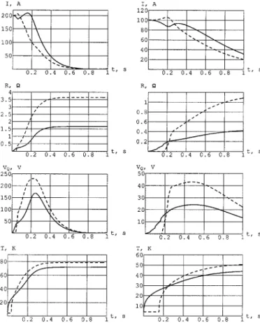
Fig. 6. (Solid line) Coil A. (Dashed line) Coil B.
A. Mass Transition of the Coil B Alone
In Figs. 3 and 4 examine the quench process of the coil B alone. The magnetic field inhomogeneity causes the normal zone to propagate faster near the inner radius of the coil. In the case of a quench starting at the bottom of the coil, a lower speed yields the final temperature to be higher than in the classical case where the quench starts at the middle of the inner radius. The Wilson’s method with ellipsoidal normal zone is not well suited to study these potentially more dangerous cases whereas our method allows us to catch the behavior of the evolving normal zone.
B. Magnet Subdivision Protection: Coils A and B
We show the influence of the initial current in a more complex example where two coils A and B are protected by subdivision (Figs. 5 and 6).
VI. CONCLUSION
We have presented a two-dimensional generalization of the Wilson’s method. This method avoids several drawbacks of the Wilson’s one using the level-set method. The method is inter-esting in the context of complex normal zone motion. The corre-sponding quench resistance and hot spot temperature are taken into account better than with the classical Wilson’s method. In future works, the ability of the method to make fast simulations will be used for superconducting coils design and protection op-timization.
REFERENCES
[1] M. N. Wilson, “Computer Simulation of the quenching of a supercon-ducting magnet,” Rutherford High Energy Physics Laboratory, Memo RHEL/M151, 1968.
[2] V. Kadambi and B. Dorri, “Current decay and temperatures during su-perconducting magnet coil quench,” Cryogenics, vol. 26, p. 157, 1986. [3] C. H. Joshi, J. E. C. Williams, and Y. Iwasa, “Quenching in epoxy impregnated superconducting solenoids: Prediction and verification,”
IEEE Trans. Magn., vol. MAG-23, pp. 922–925, 1987.
[4] D. Eckert, A. Gladun, A. Mobius, and P. Verges, “Numerical treatment of the quenching process in superconducting magnet systems,”
Cryo-genics, vol. 21, pp. 367–371, 1981.
[5] L. Turner, “Three computer codes for safety and stability of large su-perconducting magnets,” presented at the Cryogenic Engineering Conf., Cambridge, MA, Aug. 1985.
[6] S. Osher and C. Shu, “High-order nonoscillatory schemes for Hamilton–Jacobi equations,” J. Comp. Phys., vol. 28, pp. 907–922, 1991.
[7] A. Harten, B. Engquist, S. Osher, and S. Chakravarthys, “Uniformly high order accurate essentially nonoscillatory schemes. III,” J. Comp.
Phys., vol. 71, no. 2, pp. 231–303, 1987.
[8] J. A. Sethian, “Level-set methods and fast marching methods,”
Cam-bridge Monographs on Applied and Computational Mathematics, 1999.
[9] , “Curvature and the evolution of fronts,” Commun. Math. Phys., vol. 101, pp. 487–499, 1985.
[10] , “Numerical algorithms for propagating interfaces: Hamilton–Ja-cobi equations and conservation laws,” J. Differential Geometry, vol. 31, pp. 131–161, 1990.
[11] Y. Iwasa, Case Studies in Superconducting Magnets. New York: Plenum, 1994.
[12] C. H. Joshi and Y. Iwasa, “Prediction of current decay and terminal volt-ages in adiabatic superconducting magnets,” Cryogenics, vol. 29, Mar. 1989.
[13] Z. P. Zhao and Y. Iwasa, “Normal zone propagation in adiabatic super-conducting magnets.—Part 1: Normal zone propagation velocity in su-perconducting composites,” Cryogenics, vol. 31, Sept. 1991.
[14] L. Dresner, Stability of Superconductors. New York: Plenum, 1995. [15] A. V. Gurevitch, R. G. Mints, and A. L. Rakhmanov, The Physics of
Composite Superconductors. New York: Begell House, 1997. [16] A. V. Gurevitch and R. G. Mints, “On the theory of normal zone
propa-gation in superconductors,” IEEE Trans. Magn., vol. 17, Jan. 1981. [17] L. K. Urankar, “Vector potential and magnetic field of current-carrying
finite arc segment in analytical form, Part III: Exact computation for rectangular cross section,” IEEE Trans. Magn., vol. 18, Nov. 1982. [18] R. Piessens, E. de Doncker-Kapenga, C. W. Ueberhuber, and D. K.
Ka-haner, QUADPACK, A Subroutine for Automatic Integration. Berlin, Germany: Springer-Verlag, 1983.