HAL Id: hal-00773213
https://hal.archives-ouvertes.fr/hal-00773213
Submitted on 11 Jan 2013HAL is a multi-disciplinary open access
archive for the deposit and dissemination of sci-entific research documents, whether they are pub-lished or not. The documents may come from
L’archive ouverte pluridisciplinaire HAL, est destinée au dépôt et à la diffusion de documents scientifiques de niveau recherche, publiés ou non, émanant des établissements d’enseignement et de
Structural features of pyrocarbon atomistic models
constructed from transmission electron microscopy
images
Jean-Marc Leyssale, Jean-Pierre da Costa, Christian Germain, Patrick
Weisbecker, Gérard Vignoles
To cite this version:
Jean-Marc Leyssale, Jean-Pierre da Costa, Christian Germain, Patrick Weisbecker, Gérard Vignoles. Structural features of pyrocarbon atomistic models constructed from transmission electron microscopy images. Carbon, Elsevier, 2012, 50 (12), pp.4388-4400. �10.1016/j.carbon.2012.05.015�. �hal-00773213�
Structural features of pyrocarbon atomistic models
constructed from transmission electron microscopy
images
J.-M. Leyssalea,∗, J.-P. Da Costab
, C. Germainb
, P. Weisbeckera
, G. L. Vignolesc
a
CNRS, Laboratoire des Composites ThermoStructuraux, UMR 5801 CNRS-Snecma Propulsion Solide-CEA-Universit´e Bordeaux 1,33600 Pessac, France
b
Univ. Bordeaux, ENITAB, Laboratoire de l’Int´egration du Mat´eriau au Syst`eme, UMR 5218 CNRS-IPB - Universit´e Bordeaux 1, 33405 Talence, France
c
Univ. Bordeaux, Laboratoire des Composites ThermoStructuraux, UMR 5801 CNRS-Snecma Propulsion Solide-CEA-Universit´e Bordeaux 1, 33600 Pessac, France
Abstract
We report on atomistic models of laminar pyrocarbons constructed using a combination of 2D high resolution transmission electron microscopy (HRTEM) lattice fringe image analysis, 3D image synthesis and atomistic simulated an-nealing. In a first step, the effectiveness of the method and the convergence of the models with respect to the quench rate are checked on small systems. Then, the nanostructural features of large fully carbonaceous atomistic mod-els obtained from the HRTEM images of a rough laminar pyrocarbon, as-prepared and after partial graphitization, are discussed. Both models show a very pronounced sp2 character (≥ 97%), essentially made of hexagonal rings
(≥ 88%) and pentagonal and heptagonal rings in similar amounts (≈ 6%). The latter mostly form pentagon-heptagon pairs or networks of line defects
∗Corresponding author
between misoriented hexagonal domains. Numerous pairs of screw disloca-tions, connecting different graphene domains, are also observed while edge dislocations with unsaturated carbon atoms are almost absent. The mod-els are validated with respect to experimental pair distribution functions, showing excellent agreement.
1. Introduction
Low temperature pyrolytic carbons, or pyrocarbons (PyCs), as obtained from chemical vapor infiltration of fibrous preforms, are essential constituents of many high performance composite materials; such as the matrices of Car-bon/Carbon composites [1] for spatial applications or as the interphases of many SiC/SiC materials found in aeronautic or nuclear energy industries [2]. These pyrocarbons are dense sp2 carbons but, in their ”as prepared”
form, can contain large and variable amounts of defects. Different classes of PyCs, differing in their microstructure and consequently in their proper-ties (graphitizability, mechanical properproper-ties, thermal properproper-ties, etc...), have been identified [3–5] and related to the preparation conditions [6, 7]. Under-standing their structure-property relationship is a key issue in quality control as well as in designing new materials with targeted properties. Many papers have been published on the different microstructures of PyCs and their prop-erties [3–9]. However, very few of them have given a clear picture of these materials at the atomic scale (nanostructure) so far, and, for instance, the first pair distribution functions (PDFs) of PyCs have only been measured very recently [10].
and also visualize, the nanostructure of such partially disordered materials and two classes of methods, the mimetic and knowledge based approaches [11], can be used in that goal.
In the mimetic approach, atomistic models are built by simulating the synthesis process of the materials. For instance, liquid quench molecular dynamics (LQMD) simulations are often used to mimic the physical vapor deposition (PVD) of amorphous carbons [12, 13]. However, direct MD simu-lation is limited to extremely fast synthesis processes, as this technique can-not span timescales larger than a microsecond. Applying a mimetic method to a ”slow” fabrication process thus requires developping problem-specific approaches [14, 15].
In the knowledge based approach, on the other hand, no attention is paid to the history of the materials; the models are solely built on the basis of reproducing a selected set of properties. The most popular technique in that purpose is the reverse Monte Carlo (RMC) method [16]. In a RMC simula-tion, atoms, or blocks of rigidly bound atoms, are randomly moved in space and the moves are either accepted (or rejected) with a probability based on the root mean square deviation between the PDF of the model and the experimental PDF of the material. Among the recent improvements of the RMC method one can site the hybrid RMC (HRMC) method, a composite method between RMC and conventional Metropolis Monte Carlo (MC) in which an empirical reactive potential ensures the formation of properly de-fined chemical bonds in addition to the fit of the PDF [17, 18]. Also, PDF data can be complemented, or even replaced, by other sets of structural in-formation in an RMC (or HRMC) process. For instance, Nguyen et al. have
constructed models of activated carbons using a HRMC method based on the reproduction of pore size and pore wall thickness distributions [19].
In the particular case of highly textured materials, a successful knowledge based construction must be based, at least in part, on the reproduction of some nanotextural information. Lattice fringe images obtained in high resolution transmission electron microscopy experiments are often used to describe the nanotexture of dense aromatic carbons [3]. Considering this, we immediately think of an RMC (or HRMC) process in which the target experimental data would be the HRTEM image. Even though it is possible to directly simulate a HRTEM image from an atomistic configuration - it has even been done for validation purposes in some papers [20, 21] - image simulation is much too computationally expensive to be performed, say, tens of thousands times, as would be required in an RMC simulation.
Following recent progress in statistical analysis of HRTEM images [22–26] and in image synthesis techniques [27, 28] we have recently proposed a new knowledge based method, the image guided atomistic reconstruction (IGAR) method [29], aiming at building realistic atomistic models of nanotextured carbons from almost the sole knowledge of their HRTEM images and density.
This method is presented in details in section 2. Results of its application to two images of a rough laminar PyC are then presented in section 3 with a particular emphasis on both the structural features of the obtained models and on the parameters - inherent to the methodology - that can affect the quality of the resulting models. Finally we conclude in section 4 with a discussion on the ”hits and misses” of the proposed approach and of some possible ideas of improvement.
2. Methods
2.1. HRTEM-like 3D image synthesis
The first step of the IGAR method consist in building 3D analogues of the actual 2D HRTEM specimens. To do so we extend to 3D the parametric approach of Portilla and Simoncelli [27] for the synthesis of a 2D texture from a 2D exemplar. First, after being filtered with both a radial and di-rectional band-bass filter [30], them HRTEM image sample is decomposed into a pyramid of multi-resolution subbands which are then analyzed to pro-duce a pyramidal collection of 2D first order (mean, variance, skewness and kurtosis) and second order (autocorrelation coefficients) reference statistics [27]. In a second step, these 2D reference statistics are extended to produce a pyramical collection of 3D target statistics through 2D/3D statistical in-ference. This is trivial for first order statistics which are equal in 2D and 3D.
Figure 1: Filtered HRTEM image sample (a) and the chosen Cartesian (x, y, z) and spher-ical (ρ, θ, φ) coordinate systems (b).
Fig. 1 helps us in explaining how we deduce 3D autocorrelation coeffi-cients r3D(x, y, z) from the reference 2D autocorrelation coefficients r2D(x, z).
Laminar pyrocarbons are orthotropic materials: all the properties of the ma-terial (structural, mechanical, thermal, etc...) are the same whatever the direction considered provided that it is orthogonal to the orthotropy direc-tion, the stacking direction of graphene layers (vertical direction in Fig. 1a). This, of course, also holds for the properties of HRTEM images, and so r3Dsph(ρ, θ, ϕ) = r2Dpol(ρ, ϕ), whatever the value of θ (here superscripts sph and pol relate to respectively spherical and polar coordinate systems (see Fig. 1b)). It easily follows [28] that the 3D autocorrelations coefficients r3D can
be deduced from r2D by interpolation using
r3D(x, y, z) = r2D(ρ cos ϕ, ρ sin ϕ). (1)
Finally, a 3D texture, initially random, is alternately decomposed into a 3D multi-resolution pyramid, modified to meet the 3D target statistics, reconstructed, re-decomposed, etc... until convergence. At that point we dispose of a 3D analogue of the filtered experimental HRTEM image in the sense that every 2D slice of the 3D image, taken parallel to the orthotropy axis, is statistically equivalent to the latter.
2.2. Image guided atomistic reconstruction
The IGAR procedure starts with the definition, or the superposition, of a physical system on the synthesized 3D images. Basically, a physical volume, here a cube, with periodic boundary conditions (3D images are periodic as well) and edge size given by the interfringe distance of the material (d002)
associated to the image blocks. This volume is then filled with randomly located carbon atoms at the suited density. Then, we perform a simulated annealing (a ”slow” temperature quench) simulation, using either molecular dynamics (MD) or Monte Carlo (MC) sampling, in which the potential energy of the system is defined by
U = UREBO+ UHRT EM (2)
In this equation UREBO represents the interatomic potential energy, defined
by the second generation REBO potential function [31]:
UREBO = N−1 X i=1 N X j=i+1 fc(rij) [VR(rij) − bijVA(rij)] (3)
where N is the number of atoms, rij is the distance between carbon atoms
i and j, fc(r) is a switching function that goes smoothly from unity for
r = 0.17 nm to zero for r = 0.2 nm, VR(r) and VA(r) are respectively the
repulsive and attractive potentials and bij is an empirical bond order term
taking into account the local environments of atoms i and j. UHRT EM is
a fictitious interaction potential between the physical system and the 3D HRTEM image: UHRT EM = kIm N X i=1 IIm(ri) (4)
where IIm(ri) is the greyscale level, ranging from zero to one for respectively
black and white voxels, of the 3D image at position (ri) of atom i (IIm(ri)
is computed by trilinear interpolation using the greyscale levels of the eight voxels closest to location ri).
This last term is rather unusual and definitely unphysical. Its only aim is to bring the atoms to settle on the dark areas of the 3D images (the fringes). It actually acts like an external potential field imposing an experiment based property of the materials to the model, namely its nanotexture, in close sim-ilarity with the HRMC method in which the RMC part (the fit to the PDF) can be somehow considered as an external potential as well. IGAR somehow resembles the one work of Petersen et al. [32] who performed HRMC sim-ulations in which atoms were constrained on analytic surfaces derived from HRTEM observations to build atomistic models of glassy carbons. However, in the IGAR method atoms are not rigidly constrained on the fringes, al-though being attracted by the dark areas, and no PDF data are used in the model construction process, unlike what is done in most RMC methods.
Also, we can note a certain similarity between the IGAR approach and the templating approach of Roussel et. al. [15]. Indeed, while they simulate the equilibrium between an ideal carbon gas and the carbon phase sorbed in the zeolite, or in other words the carbon gas in presence of the ”external” potential field created by the zeolite, we simulate the quench of a carbon liquid in presence of an external potential field created by the 3D HRTEM image.
There are three ”user-defined” parameters in the IGAR procedure: (i) the initial temperature of the system T0; (ii) the rate (in K/s or K/MC
attempt for simulated annealing performed with respectively MD or MC simulations) at which the system is cooled down to zero temperature; and (iii) the proportionality factor kIm between grey level and energy. In order
be chosen so that the system at this temperature is diffusing (liquid). The quench rate has to be chosen as slow as possible to ensure convergence of the final configurations, in terms of energies and structure, while remaining computationally affordable. Finally, kIm has to be strong enough to impose
the suited nanotexture while being as low as possible in order not to affect the chemical quality of the models (here we remember that UREBO is physical,
UHRT EM not).
2.3. Simulation details
Two experimental HRTEM images taken from the matrices of C/C com-posites were considered (see Fig. 2a and b). They correspond respectively to a rough laminar PyC, as prepared (AP) and after heat treatment (HT) inducing a partial graphitization. These images, on which the 2D analy-sis is performed have been choosen from the domains with highest contrast among larger samples, to insure the best possible alignment with regards to the Scherzer focus and Eucentric position, although our aim here is mainly to discuss the similarities and differences between such an AP and HT ma-terials and not to quantitatively characterize the two individual mama-terials.
From these 2D images, four 3D cubic image blocks, 128 × 128 × 128 voxels each were obtained through the 2D analysis - 3D synthesis image processing scheme described in section 2.1. The first two (one for each material) are small images, 13 fringes high on average along the orthotropy axis, aimed at finding the most suitable cooling sequence and optimum value of kIm. The
other two, counting on average respectively 16 and 17 fringes for respectively the AP and HT PyCs (see Fig. 2e and f), are then used in order to build models of sufficient size to capture the nanostructural differences between
the two materials. The steerable pyramid decomposition, used in the image analysis synthesis step, was performed with 3 levels and 4 orientations and autocorrelation coefficients were taken on 7×7 neighborhoods. Ten iterations were enough to converge towards stable 3D textures. Then, the resolution of the synthesized textures was improved to 512 × 512 × 512 through spline interpolation before feeding the IGAR code.
In the IGAR procedure, we consider the materials as entirely made of carbon atoms (ideally around one atomic percent of hydrogen should be considered as well [10]) with an equal density of 2.1 g/cm3 (a higher (resp.
lower) limit for the AP (resp. HT) PyC). We also use the same value for the interlayer distance d002 = 0.35 nm. This value is typical for an AP PyC
and slightly too high for the HT PyC, however, our point here is to focus on the structural differences induced by different nanotextures, everything else being equal. With these parameters we built initial atomistic configurations of 9926 atoms in a cubic box of 4.55 nm edge for the two small images and boxes of 18507 and 22198 atoms (cubes of 5.6 and 5.95 nm edges) for respectively the large 16 fringes AP and 17 fringes HT systems. Atoms were randomly inserted in the volumes with a non-overlap condition of 0.13 nm to ensure a reasonable initial energy.
As a sampling technique we chose an isothermal NV T MD algorithm based on the stochastic thermostat proposed by Andersen [33]. In this method, Newton’s equations of motion
˙ri = pi/mi (5)
and
(where ri, pi and mi are respectively the position, momentum and mass of
particle i, U is the total potential energy defined in Eq. 2 and ∇i indicates
the derivative with respect to ri) are numerically integrated using the velocity
Verlet algorithm [33] with a 0.2 fs timestep. After each step, every atom has a 0.2 % probability to have its velocity redrawn from a Maxwell-Boltzmann distribution corresponding to the target temperature. The simulated anneal-ing is performed by changanneal-ing (loweranneal-ing) this target temperature at every step according to a predefined cooling sequence.
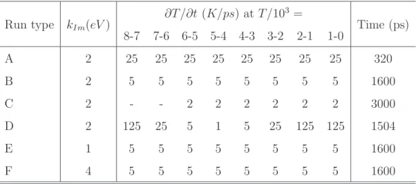
Table 1: Summary of the different combinations of quench rates (∂T /∂t) and kI m used
in IGAR simulations performed on small (13 fringes) 3D image blocs (the total simulated time is also indicated).
Run type kIm(eV )
∂T /∂t (K/ps) at T /103 = Time (ps) 8-7 7-6 6-5 5-4 4-3 3-2 2-1 1-0 A 2 25 25 25 25 25 25 25 25 320 B 2 5 5 5 5 5 5 5 5 1600 C 2 - - 2 2 2 2 2 2 3000 D 2 125 25 5 1 5 25 125 125 1504 E 1 5 5 5 5 5 5 5 5 1600 F 4 5 5 5 5 5 5 5 5 1600
Three different values of kIm: 1, 2 and 4 eV, and different cooling
se-quences were tested on the small 13 fringes image blocks as summarized in table 1.
2.4. Structural analysis
Once the IGAR simulation has been performed, and prior to structural analysis, a short (typically 100 ps) MD simulation is performed at 300 K us-ing the AIREBO potential [34] to relax the structure (note that it is achieved only on the large atomistic models, not on the small systems used in section 3.2). This potential is a modification of the REBO potential including an adaptive treatment of van der Waals interactions between non-bonded atoms. Obviously, the image potential is switched off during this relaxation simu-lation. At that point, many structural properties of the resulting models are computed. It includes the usual average coordination numbers and bond angle distributions where two atoms form a bond if they are distant by less than 1.85 ˚A (an intermediate value between first and second neighbours in graphene).
From that, ring statistics can be computed using the ”shortest path ring” algorithm of Franzblau [35] where only threefold atoms are taken into ac-count. To go a little further than the simple ring statistics, we have also developed a clustering approach to determine those threefold atoms belong-ing only to hexagonal rbelong-ings (called pure C6 atoms) and among them those
atoms belonging to rings entirely made of pure C6 atoms (noted pure C6
rings). Finally, fragments, or clusters of rings, are defined on the basis that two pure C6 rings sharing an atom belong to the same fragment. This
algo-rithm is essentially the same as the one of Jain and Gubbins [36] except that only threefold atoms and hexagonal rings are considered.
HRTEM images of the PyC models are simulated using the multislice sim-ulation approach as implemented in the NCEMSS software package [37]. In
those simulations we adopted typical microscope parameters used to produce experimental images of PyC matrices: Philips CM30ST microscope with a 300 kV accelerating voltage, Scherzer defocus of -58 nm, spread of defocus of 7 nm, spherical aberration (Cs) of 1.2 mm, convergence angle of 0.5 mrad
and aperture radius of 4 nm−1.
Finally, the reduced pair distribution functions (PDFs), defined as
G(r) = 4πρr [g(r) − 1] (7)
where ρ is the atomic density and
g(r) = 1 4πr2ρN * N X i=1 N X j6=i δ (r − rij) + (8) is the atomic pair distribution function (where N is the number of atoms and δ (r − rij) = 1 when atoms i and j are distant by r and 0 otherwise), were
computed from a statistical averaging on an equilibrated MD simulation at 300 K.
3. Results
3.1. Synthetic 3D HRTEM-like images
The experimental HRTEM images of the AP (Fig. 2a) and HT (Fig. 2b) PyCs are shown after high and low frequency filtering on Figs 2c and 2d respectively. As compared to the raw images, we can see that the filtered images only contain the fringe characteristics, namely, their length, curva-ture, contrast, etc ... More specifically, we see that fringes of the AP PyC are neatly shorter, more curved and more interconnected than those of the HT PyC.
Figure 2: Illustration of the 3D HRTEM-like images synthesis. Experimental HRTEM image of a PyC as prepared (AP)(a) and heat treated (HT)(b); Filtered HRTEM image of a PyC AP (c) and HT (d); Synthesized 3D HRTEM-like image of a PyC AP (e) and HT (f). Images (a, c and e) counts on average 16 fringes in the stacking direction against 17 fringes for images (b, d and f).
3D views of the synthesis results are shown in Fig. 2e and f. Percep-tually speaking, the two solid textures are quite convincing. They are free from major artifacts. 2D slices of these solid textures show morphological properties close to the ones observed in the corresponding filtered HRTEM images: straight and distorted fringe lengths and curvatures are similar. The overall anisotropy seems to be respected as discussed in [28]. Fringe lengths and tortuosities calculations would allow for a more thorough comparison, however the size of the synthesized blocks, only of around 6 nm, does not allow yet for such a study; this will be achieved in the future on larger blocks. 3.2. Preliminary study on a 13 fringes AP PyC
We start the IGAR study by searching for the best cooling sequence and the best value of kIm using a 13 fringes image block synthesized from the
HRTEM image of an AP PyC. This preliminary study is presented in more details in the first section of the supporting material and we only discuss here the main results. The final properties (UREBO, UHRT EM, coordination data
and ring statistics) of models constructed using IGAR simulations with the six sets of parameters of table 1 are summarized in table 2.
We can see in table 2 that, among the six model constructions, run D is the one that results in the lowest value of UREBO, the largest sp2 fraction
and the largest amount of six-membered rings, while keeping a low value of UHRT EM/kIm. It is thus the best combination of quench algorithm and kIm.
Note the particular interest of the ramp cooling sequence, which performs better than a uniform cooling at 2K/ps with the same value of kIm despite
being twice shorter in terms of computer time. As a consequence, IGAR parameters of run D will be used in what follows to build large AP and HT
Table 2: Final properties of 13 fringes AP PyC models.
Run A B C D E F
kIm(eV ) 2 2 2 2 1 4
Quench rate (K/ps) 25 5 2 ramp 5 5
UREBO(eV ) -7.132 -7.209 -7.236 -7.239 -7.200 -7.192 UHRT EM/kIm 0.307 0.305 0.305 0.305 0.322 0.294 sp fraction 0.007 0.004 0.003 0.003 0.002 0.007 sp2 fraction 0.951 0.965 0.970 0.970 0.961 0.966 sp3 fraction 0.042 0.031 0.027 0.027 0.037 0.027 C5 fraction 0.142 0.093 0.069 0.058 0.109 0.092 C6 fraction 0.689 0.801 0.852 0.875 0.755 0.806 C7 fraction 0.143 0.100 0.077 0.063 0.122 0.094 C8 fraction 0.015 0.004 0.002 0.004 0.011 0.007
PyC models.
3.3. Atomistic pyrocarbon models
3.3.1. General structural features
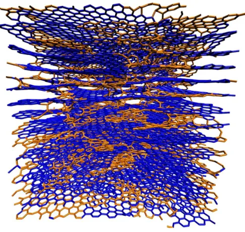
The IGAR procedure is now applied to the 16 fringes image block of the AP PyC (Fig. 2e) and to the 17 fringes image block of the HT PyC (Fig. 2f). Snapshots of the models obtained for these two materials, after a short MD relaxation at 300 K using the AIREBO potential, are shown in respectively Fig. 3 and Fig. 4. Their main structural parameters are given in table 3 (a movie, illustrating the construction of the AP PyC model is also given as supporting material, section 2).
Confirming the studies on smaller systems presented earlier, both models are typical of sp2
graphitic carbons (mostly 3-fold C atoms and C6 rings).
They also contain similar amounts of pentagonal and heptagonal rings, 5-6 % for both models and a few octagonal rings (0.2-0.3 %). Also, in agreement with the high fractions of hexagonal rings, the fractions of pure C6 atoms
(fatom
pC6 ) and of pure C6 rings (f
rings
pC6 ) are high for both models. Some years
ago Vallerot et al. [5] have reported on angle resolved electron energy loss spectroscopy (EELS) experiments to assess the hybridization of PyC matri-ces. Their results indicate that RL PyCs contain 82.5 % of pure sp2 carbons,
the remaining atoms having, according to them, a sp2+ε hybridization, due
to out-of-plane distorsions as well as some C7/C5 rings. They also claim than
sp3
hybridization should be very small in these materials as confirmed by the very weak Raman D band and by the fact that a significant amount of sp3
carbon atoms in such low nanoporosity materials would be incompatible with their densities of around 2.1 g/cm3. Our models comprising 97 and 99 % of
Figure 3: Snapshot of the 16 fringes AP PyC model. Bonds between carbon atoms belonging to pure hexagonal domains are shown with blue sticks. Other C-C bonds are shown with orange sticks.
Table 3: Final properties of PyC models constructed from a 16 fringes AP PyC image and a 17 fringes HT PyC image (a 2 eV value of kI mwas used with the ramp cooling algorithm).
Material UAIREBO fsp fsp2 fsp3 fC 5 fC6 fC7 fC8 f atom pC6 f ring pC6 AP -7.283 0.005 0.973 0.022 0.054 0.886 0.057 0.003 0.753 0.700 HT -7.300 0.002 0.990 0.008 0.054 0.889 0.055 0.002 0.764 0.737 20
threefold atoms for respectively the AP and HT PyCs are totally compatible with the latter assumption. Moreover, the fractions of pure C6 atoms
(re-spectively 75 and 76 % for the AP and HT PyCs) and pure C6rings (70 % for
AP, 74 % for HT) are not far from the 82.5 % pure sp2 atoms measured by
these authors and our models suggest that the ”sp2+ε” hybridization would
actually essentially be due to non-hexagonal rings.
Even though the presented coordination and ring statistics are interest-ing and compatible with experimental observations, these properties, mainly characterizing short-range order in the materials, are unable to unambigu-ously discriminate between the AP and HT PyCs. Nevertheless, and as expected for pyrocarbons, they differ considerably from data reported for atomistic models of more disordered carbons like chars [38], saccharose based carbons [17, 36] and glassy carbon [18], constructed using HRMC methods. Indeed, those models show much lower sp2 contents (between 50 and 90 %)
and fractions of hexagonal rings.
The bond angle distributions shown in Fig. 5 show two very similar curves, almost indistinguishable from each other, and narrowly peaked around the 120 ◦ angle of the honeycomb lattice for both the AP and HT models.
They are only slightly broader than the corresponding distribution for hexag-onal graphite due to the existence of sp3carbon atoms and C
5rings (low angle
broadening) as well as C7 and C8 rings (large angle broadening). Again, bond
angle distributions reported for atomistic models of more disordered carbons [18, 38] are much broader than the ones reported here for PyCs.
As has been quantified, the two models are essentially the same at very short range, typically at the length scale of one (or a few) chemical bond(s).
Figure 5: Room temperature bond angle distributions of the 16 fringes AP model (squares), the 17 fringes HT model (circles) and hexagonal graphite (dotted line) as ob-tained from MD simulations.
Moreover, looking at Fig. 3 and 4, we see that they are both made of some nanosized pure hexagonal domains made of pure C6 rings (blue), connected
together by defect containing domains (orange). However, these figures also clearly highlight some differences in their nanotextures, as discussed here-after.
3.3.2. Out-of-plane defects features
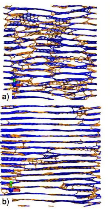
Looking at Fig. 4 we can see that the HT model is characterized by extended, and rather flat, carbon sheets, with few interconnections. The AP model (see Fig. 3), on the other hand seems to present smaller and more curved sheets with numerous interconnections along the stacking direction. These differences are clearly confirmed in Figure 6, showing 2-nm thick slices of the models, taken along the stacking direction. Indeed, in the case of the HT PyC (Fig. 6b) some well defined flat domains, extending on the whole width of the simulation box (5.95 nm), are neatly visible; in the AP PyC model (Fig. 6a), such domains roughly never exceed 2 nm.
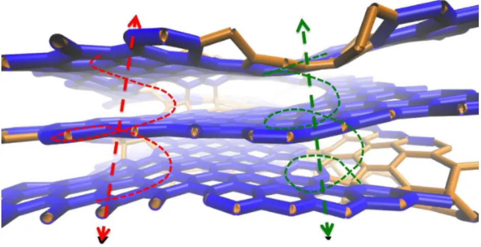
Fig. 7 shows a chunk of the AP model, highlighting the screw dislocation structure of this material. As can be seen, those domains remind us of the shape of the access ramp in multi-floors car parks. Moreover, as shown in the hexagon preserving carbon nanofoams predicted some years ago by Kuc and Seifert using density functional tight binding calculations [39], these disloca-tions can be well accommodated by pure hexagonal sp2 carbon structures;
this is almost the case of the dislocation appearing on the top right corner of Fig. 7. Such screw dislocations are also found in the HT model, yet in much lower amount.
Figure 6: 2 nm-thick slices of the AP (a) and HT (b) models (same color code as in Figures 3 and 4).
Figure 7: Chunk of the AP PyC model showing a screw dislocation pair (red and green dashed lines and arrows; chemical bonds are displayed with the same color code as in Fig. 3 and 4).
3.3.3. In-plane defects features
We show in Fig. 8 two carbon sheets taken from the models. Common to the two models, and as already said below, the sheets contain nanosized domains entirely made of sp2
pure C6 rings (in blue). These domains are
connected together by disordered areas (orange) and by screw dislocations (holes). More precisely, the disordered areas, in agreement with data from table 3, are essentially made of C5, C7 and ”non pure” C6 rings (i.e. C6
rings containing at least an atom that is not threefold or that also belongs to another kind of ring) as well as a few fourfold or twofold atoms and C8
rings. Nevertheless, those areas are not as ”disordered” as we could think at first sight. Indeed, as shown with red lines on Fig. 8, C5 and C7 rings
Figure 8: Carbon sheets (0.3 nm-thick in-plane slices) of the AP (a) and HT (b) PyC models (same color code as in Figures 3 and 4; red lines indicate the pentagon/heptagon pairs and lines of pairs).
lines or networks of C5/C7 pairs. This is in agreement with recent theoretical
works on non-hexagonal ring defects in graphene, showing the high stability of defects based on the C5/C7 pattern [40–42]. Also, it is important to note
that we did not observe any isolated pentagon, a defect associated to highly curved structures like fullerenes, glassy carbons or other non graphitizing carbons [43, 44]. Comparing now Fig. 8a and b allows confirming some previous remarks, namely that the AP model presents more dislocations and more wavy sheets than the HT model. Also, as we can see in these figures, if the AP model shows only isolated C5/C7 pairs or very short C5/C7 lines,
the HT model on the opposite shows rather extended lines, made of up to six or seven C5/C7 pairs.
In order to understand a little further the role played by these disordered domains, and their origin, we show in Fig. 9 three portions of carbon sheets taken from the HT model. As we can see in the three panels of this figure, these extended C5/C7 lines actually act as grain boundaries between
disori-ented hexagonal domains. We can guess that the hexagonal domains form first and that the networks of pentagons and heptagons develop themselves when these hexagonal domains with different ”in-plane” orientations merge. Also, a few interesting features can be observed on these figures. First, as highlighted by a green circle, a Stone-Thrower-Wales defect is clearly visible in Fig. 9a. Second, the disordered area of Fig. 9b, almost circular, surrounds a very small hexagonal domain with a different orientation than the rest of the sheet. Finally, the pentagon and heptagon containing area delimited by the green rectangle on Fig. 9c is particularly interesting. Indeed, this domain is space-filling, meaning that entire sheets can be made out of its repetition
Figure 9: Snapshots of some carbon sheets taken from the HT model (same color code as in Fig. 8; orientations of some hexagonal domains are indicated by dashed black arrows, a Stone-Thrower-Wales defect and a C2
5C 3 6C
2
7 defect, studied in details elsewhere [45], are
by translation. The structure and properties of nanocarbons based on it (sheets and tubes) have been studied elsewhere [45].
In an attempt to quantify the structural differences between the two ma-terials at the mesoscale we have performed a cluster analysis of pure C6rings.
Fig. 10 gives histograms of the different fragments (clusters of connected pure C6 rings) found for these models. As can be seen on the upper panel of Fig.
10, the AP model counts much more very small fragments than the HT one, for instance, 17 isolated pure C6rings are found in the AP model against 3 in
the HT model (note that according to our definition, an isolated pure C6 ring
actually means a C6 ring surrounded by six non pure C6 rings). The
struc-ture of the AP Pyc can actually be discribed by a combination of very small ”mono-sheet” fragments of less than 80 pure C6 rings and two very large
”multi-sheets” fragments counting for more than 90 % of the pure C6 rings
present in the model which indicates a very high density of screw dislocations (a graphite sample of similar dimensions would be made of grephene sheets of only 620 rings).On the opposite, the HT PyC is made of larger mono-sheet fragments, indicating a better ”in-plane” order, and smaller ”multi-sheet” fragments, indicating a lower density of dislocations.
3.3.4. HRTEM validation
In order to verify that our models actually corresponds to the experi-mental materials we now compare the experiexperi-mental HRTEM images to those simulated from the models using the multi-slice method [37]. Fig. 11 shows the experimental HRTEM images of AP (Fig. 11a) and HT (Fig. 11b) PyCs after high and low frequency filtering (identical to Figs 2c and 2d), together with the images simulated from the AP (Fig. 11c) and HT (Fig. 11d)
atom-Figure 10: Histogram of the number of fragments found in the AP (red filled bars) and the HT (green empty bars) models with respect to their size (in terms of the number of pure C6 rings (the histogram is split into three panels according to the fragment size; small
fragments: top, large fragments: bottom; numbers in the panels indicate the fragments sizes in atoms).
Figure 11: Comparison between experimental and simulated HRTEM images. a: filtered experimental image of the AP PyC (equivalent to Fig. 2c); b: filtered experimental image of the HT PyC (equivalent to Fig. 2d); c: simulated image from the AP model; d: simulated image from the HT model.
istic models.
Bearing in mind that the 3D image blocks guiding the IGAR simulations are not directly inferred from 2D images but from statistical descriptors of these images, images simulated from the model do not have to be identical replicas of experimental images but statistically equivalent to them (espe-cially second order statistics, describing the fringes properties, while first order statistics are more sensitive to the parameters governing the virtual microscope in the image simulation process). Looking at Fig. 11 we can see that apart from differences in contrast, the similarity in terms of fringes undulations and junctions, between initial images (Fig. 11a and 11b) and their corresponding simulated images (Fig. 11c and 11d) is obvious and con-firm that the atomistic models contain most of the nanotextural information present in the HRTEM images.
Fig. 12 presents the gradient orientation maps computed from the HRTEM images of Fig. 11. In such an image, a red pixel indicates a zone with a ver-tical gradient, i. e. a horizontal fringe characterizing a graphitic order, and yellow/blue pixels correspond to areas with horizontal gradients (defective domains/stacking faults). Comparing Fig. 12a to 12c confirms that the ex-perimental (Fig. 11a) and simulated (Fig. 11c) HRTEM images of the AP material present similar defects, both in terms of density and extent. A similar observation can be made for the HT material (see the good match between Fig. 12b and d). Obviously, images from the AP PyC (Fig. 12a and c) show higher amounts of defects (and more extended defects) than the HT images (Fig. 12b and d). Also, it is interesting to notice the close similarities between the fringes observed for the AP PyC (Fig. 11a or 11c) and the bond
Figure 12: Orientation maps of PyCs HRTEM images. a, b, c and d respectively show maps of the gradient orientations of Fig. 11a, b, c and d; red: vertical gradient, blue or yellow: horizontal gradient.
network of the AP model (Fig. 6a) on one side, and between the fringes of the HT PyC (Fig. 11b or 11d) and the bond network of the HT model (Fig. 6b) on the other side. For instance, the many screw dislocations observed in the atomistic model of the AP PyC (see Fig. 6a) seem to correspond pretty well to the blurred domains of the simulated HRTEM image for this model (Fig. 11c) or the defects observed on the corresponding orientation map (Fig. 12c). This can be also visualized in the supporting material movie (S2).
3.3.5. Pair distribution functions
We plot in Fig. 13 the reduced pair distribution functions computed in the range [0:30 ˚A] for the AP and HT models (the functions are split into three panels according to the interatomic distance, for clarity). Very recently, we have been able to prepare a bulk sample of rough laminar pyrocarbon. Its reduced PDF, G(r), measured using neutron powder diffraction, is also shown in Fig. 13. All details regarding this material can be found in a recent publication [10]. We add that it resides at the high anisotropy and low defect corner of the RL PyC domain in the Raman-based classification of Bourrat et al. [7] and that its nanotexture, as observed in HRTEM, seems to be intermediate between the ones of the AP and HT PyCs.
We can see in Fig. 13 that every experimental peak is present in both the AP and HT models whatever the interatomic distance r and apart from unphysical oscillations due to the Fourier transform of S(Q) (see the exper-imental function between 0 and 1.3 ˚A). The superimposition of model and experimental PDFs is especially impressive for short interatomic distances (top panel) where only slight differences can be noted: (i) the model PDFs show thinner peaks than the experimental one up to 5 ˚A and (ii) the HT
Figure 13: Reduced pair distribution function (G(r)) of the AP (solid blue line) and HT (dashed red line) PyC models. The experimental G(r) of a rough laminar PyC (PyC-1 in Ref [10]) is also shown as a filled curve for comparison (note that the functions are split into three panels (top: [0:10 ˚A]; middle: [10:20 ˚A]; bottom [20:30 ˚A] for clarity).
model has very slightly thinner peaks than the AP model. Moving to the central panel of Fig. 13 confirms the previous story though unraveling that peak locations seem to be a little shifted (actually, scaled, as we will see) to higher distances when comparing model PDFs to the experimental one, peaks of the HT model being the most shifted ones. Looking more closely at short r values, we find first neighbors peaks at respectively 1.42, 1.44 and 1.44 ˚A for the experimental function, the AP model and the HT model. Second neighbors peaks appear at 2.46, 2.47 and 2.47 ˚A (same order) and third neighbors peaks at 2.83, 2.86 and 2.87 ˚A. Scaling r values of the model PDFs by respectively 0.995 and 0.989 actually allows for an almost perfect match of the peaks locations on the whole r range (see the third section of the supported material for an ”r-scaled” version of Fig. 13).
The too low thicknesses of the peaks at short r together with their shifts to larger r at long distances are typical signatures of tensile stress in the material. Computing the stress tensors of the relaxed models we indeed find tensile in-plane stresses of around 22 and 26 GPa for respectively the AP and HT models (full stress tensors are given in the fourth section of the sup-porting material). These stresses are actually artefact due to the use of the AIREBO potential. Indeed this potential underestimate the carbon-carbon bond length in aromatic rings and simulation of graphite at experimental density give rise to a similar tensile stress with 17 GPa in-plane components. Computing the model’s properties with this potential actually leads to com-puting the properties of stressed PyCs. Using the REBO potential would avoid this artefact but in this latter case many-properties would be unrea-sonnable, especially those influenced by out-of-plane vibrations, due to the
absence of van der Waals interactions.
Figure 14: rG(r) (top) and r2
G(r) functions of the PyC models and of a real PyC. Same color code as Fig. 14.
Finally, we plot on Fig. 14 the rG(r) (14a) and r2G(r) (14b) functions
of the two models and the experimental functions of a RL PyC [10]. These two figures confirm that both models reproduce reasonably well the Neutron diffraction data and that somehow, especially when looking at intermedi-ate interatomic distances (from 5 to 25 ˚A), the experimental curves of G(r),
rG(r) and r2G(r) lie in between the ones of the AP and HT models,
confirm-ing the impression from HRTEM observations. Also, lookconfirm-ing at Fig. 14b, we see that both models have the ”right arrow with constant tail” envelope of r2G(r), which, according to us, is a specificity of rough laminar pyrocarbons
[10].
4. Conclusion
The image guided atomistic reconstruction (IGAR) method aiming at building realistic models of nanotextured carbons from experimental HRTEM imaging, image processing and atomistic simulation, has been presented in details. After discussing methodological aspects, both in terms of the tech-nique itself and of the tunable parameters inherent to the approach (quench rate, balance between image and interatomic interactions), this method has been applied to build models based on images taken from a rough lami-nar pyrocarbon matrix of a C/C composite, as prepared and heat treated. The structural similarities and differences between the two models have been carefully exposed. In particular, this work confirms a common idea on PyCs, namely that they are essentially made of nanosized aromatic domains packed together in turbostratic arrangements (the BSUs of Oberlin [3]). It also shows that the different sheets of a stack are probably connected to each other (and to those of neighboring stacks) through many screw dislocations in a kind of ”car park access ramp” arrangement. This work also shows that the main source of defects in these materials (apart from the screw disloca-tions) is not sp3 carbon atoms as one could first think but non-hexagonal sp2
with sheets of relatively low curvatures, pentagons and heptagons (especially pentagons actually) are not found as isolated defects but usually merge as pentagon/heptagon pairs, as well as lines or networks of pentagon/heptagon pairs, defining some kind of intrasheet grain boundaries between disoriented aromatic domains. Although the differences between the structures of the AP and HT models have been here mainly discussed on a qualitative basis, it seems to come out that the HT model shows larger monolayer aromatic domains, larger pentagon/heptagon networks and fewer dislocations.
It is important to recall here that the results presented here are just a first attempt to determine the structure of such complex materials at the atomic scale and that they are probably not definitive results for AP and HT rough laminar PyCs. There is surely a lot of room for improving the IGAR approach and, for instance, work is already in progress to lower the quench rates, and so improve the convergence of the models, by optimizing and parallelizing the code. Also, we are working at including given amounts of hydrogen in the models. Nevertheless, the comparison of the pair dis-tribution functions computed from these models to the data obtained using neutron powder diffraction on a rough laminar PyC sample clearly validates the interest of image guided approaches. Indeed, the agreement between the modeled and experimental G(r), rG(r) and r2G(r) is particularly good,
taking into account that the models have been constructed from only the HRTEM images of the materials and a few, easy to access, experimental data (the density and d002). In other words, the IGAR approach is able
to build a proper structural model of the material from information on its nanotexture only. Other approaches, like the RMC method, usually fail in
finding a unique nanotexture from structural experimental data (compare for instance the work of Acharya et al. [46] and Smith et al. [43] who have pro-posed drastically different atomistic models yet reproducing the same PDF data of a nanoporous carbon[47]). We add that, very recently, some atom-istic models of soot particles have been proposed through identification of fringes by pattern recognition techniques on HRTEM images, extension to 3D and replacement by polycyclic aromatic molecules [48]. This approach is interesting as it allows to generate models of very disordered materials while at present time the IGAR method requires some particular symmetry in the system to produce 3D image blocks from 2D experimental images. Also the atomistic construction in this method is probably much less costly than the very long liquid quench simulations required in the IGAR method. On the opposite, in the IGAR method, no constraint exists on the chemical nature of the material: atoms just locate themselves in space to form the lowest energy structure for a given nanotexture, thanks to the 3D image and the interatomic potential. Finally, if the first interest of the IGAR method is to produce atomistic models, allowing for a subsequent evaluation of many of their physico-chemical properties (mechanical, thermal, et...), this approach can also allow investigating the relationship between the atomistic structure and the image properties (see for instance our qualitative discussion, at the end of section 3.3.4, on the relationship between the screw dislocations ob-served in the AP model and the blurred areas obob-served in the corresponding simulated images). This will be investigated more thoroughly in future work.
Acknowledgements
Funding from the Agence Nationale de la Recherche through the Pyro-MaN project (contract ANR-2010-BLAN-929) and from the Institut Carnot Materials and systems Institute of Bordeaux (MIB) are gratefully acknowl-edged.
References
[1] Manocha LM, Fitzer E. Carbon reinforcements and C/C composites 1st ed. Berlin: Springer; 1998.
[2] Naslain R. Design, preparation and properties of non-oxide CMCs for application in engines and nuclear reactors: An overview. Compos Sci Technol. 2004;64(2):155–70.
[3] Oberlin A. Pyrocarbons. Carbon. 2002;40:7–24.
[4] Reznik B, H¨uttinger KJ. On the terminology for pyrolytic carbons. Carbon. 2002;40(4):617–36.
[5] Vallerot JM, Bourrat X, Mouchon A, Chollon G. Quantitative struc-tural and texstruc-tural assessment of laminar pyrocarbons through Raman spectroscopy, electron diffraction and few other techniques. Carbon. 2006;44(9):1833–44.
[6] Dong GL, H¨uttinger KJ. Consideration of reaction mechanisms leading to pyrolytic carbon of different textures. Carbon. 2002;40(14):2515–28. [7] Bourrat X, Langlais F, Chollon G, Vignoles GL. Low temperature
[8] Reznik B, Gerthsen D, H¨uttinger KJ. Micro- and nanostructure of the carbon matrix of infiltrated carbon fiber felts. Carbon. 2001;39(2):215– 29.
[9] Bourrat X, Lavenac J, Langlais F, Naslain R. The role of pentagons in the growth of laminar pyrocarbon. Carbon. 2001;39(15):2369–86. [10] Weisbecker P, Leyssale JM, Fischer HE, Honkim¨aki V, Lalanne M,
Vig-noles GL. Microstructure of pyrocarbons from pair distribution function analysis using neutron diffraction. Carbon. 2012;50(4):1563–73.
[11] Biggs MJ, Buts A. Virtual porous carbons: what they are and what they can be used for. Mol Sim. 2006;32(7):579–93.
[12] Marks NA, McKenzie DR, Pailthorpe BA, Bernasconi M, Parrinello M. Microscopic structure of tetrahedral amorphous carbon. Phys Rev Lett. 1996;76:768–71.
[13] Marks NA, Cooper NC, McKenzie DR, McCulloch DG, Bath P, Russo SP. A comparison of density functional, tight-binding and empiri-cal methods for the simulation of amorphous carbon. Phys Rev B. 2002;65:075411.
[14] Kumar A, Lobo RF, Wagner NJ. Porous amorphous carbon mod-els from periodic Gaussian chains of amorphous polymers. Carbon. 2005;43:3099–111.
[15] Roussel T, Didion A, Pellenq RJM, Gadiou R, Bichara C, Vix-Guterl C. Experimental and atomistic simulation study of the structural and
adsorption properties of Faujasite zeolite-templated nanostructured car-bon materialst. J Phys Chem C. 2007;111(43):15863–76.
[16] McGreevy RL, Pusztai L. Reverse Monte Carlo simulation: A new technique for the determination of disordered structures. Mol Sim. 1988;1:359–67.
[17] Jain SK, Pellenq RJM, Pikunic JP, Gubbins KE. Molecular modeling of porous carbons using the hybrid reverse Monte Carlo method. Langmuir. 2006;22(24):9942–8.
[18] Petersen TC, Yarovsky I, Snook IK, McCulloch DG, Opletal G. Struc-tural analysis of carbonaceous solids using an adapted reverse Monte Carlo algorithm. Carbon. 2003;41(12):2403–11.
[19] Nguyen TX, Cohaut N, Bae JS, Bhatia SK. New method for atomistic modelling of the microstructure of activated carbons using hybrid reverse Monte Carlo simulation. Langmuir. 2008;24(15):7912–22.
[20] Pikunic J, Clinard C, Cohaut N, Gubbins KE, Guet JM, Pellenq RJM, et al. Structural modeling of porous carbons: constrained reverse Monte Carlo method. Langmuir. 2003;19(20):8565–82.
[21] Palmer JC, Llobet A, Yeon SH, Fischer JE, Shi Y, Gogotsi Y, et al. Mod-eling the structural evolution of carbide-derived carbons using quenched molecular dynamics. Carbon. 2010;48(4):1116–23.
[22] Palot´as AB, Rainey LC, Feldermann CJ, Sarofim AF, Vander Sande JB. Soot morphology: An application of image analysis in high-resolution transmission electron microscopy. Micros Res Tech. 1996;33(3):266–78.
[23] Shim HS, Hurt RH, Yang NYC. A methodology for analysis of 002 lattice fringe images and its application to combustion-derived carbons. Carbon. 2000;38(1):29–45.
[24] Rouzaud JN, Clinard C. Quantitative high-resolution transmission elec-tron microscopy: a promising tool for carbon materials characterization. Fuel Process Technol. 2002;77-78:229–35.
[25] Germain C, Da Costa JP, Lavialle O, Baylou P. Multiscale estimation of vector field anisotropy application to texture characterization. Signal Process. 2003;83(7):1487–503.
[26] Vander Wal RW, Tomasek AJ, Pamphlet MI, Taylor CD, Thompson WK. Analysis of HRTEM images for carbon nanostructure quantifica-tion. J Nanopart Res. 2004;6:555–68.
[27] Portilla J, Simoncelli EP. A parametric texture model based on joint statistics of complex wavelet coefficients. Int J Comput Vis. 2000;40(1):49–71.
[28] Da Costa JP, Germain C. Synthesis of solid textures based on a 2D example: application to the synthesis of 3D carbon structures observed by transmission electronic microscopy. In: Proceedings of SPIE, the International Society for Optical Engineering;. .
[29] Leyssale JM, Da Costa JP, Germain C, Weisbecker P, Vignoles GL. An image guided atomistic reconstruction of pyrolytic carbons. App Phys Lett. 2009;95(23):231912.
[30] Da Costa JP, Germain C, Baylou P, Cataldi M. An image analysis ap-proach for the structural characterization of pyrocarbons. In: Proceed-ings of the International Conference on Composite Testing and Model Identification (CompTest 2004). Bristol, UK; 2004. .
[31] Brenner DW, Shenderova OA, Harrison JA, Stuart SJ, Ni B, Sinnott SB. A second-generation reactive empirical bond order (REBO) po-tential energy expression for hydrocarbons. J Phys: Condens Matter. 2002;14(4):783–802.
[32] Petersen TC, Snook IK, Yarovsky I, McCulloch DG, O’Malley B. Curved-surface atomic modeling of nanoporous carbon. J Phys Chem C. 2007;111(2):802–12.
[33] Allen MP, Tildesley DJ. Computer Simulation of Liquids. Oxford Uni-versity Press; 1987.
[34] Stuart SJ, Tutein AB, Harrison JA. A reactive potential for hydrocar-bons with intermolecular interactions. J Chem Phys. 2000;112(14):6472– 86.
[35] Franzblau DS. Computation of ring statistics for network models of solids. Phys Rev B. 1991;44(10):4925–30.
[36] Jain SK, Gubbins KE. Ring connectivity: measuring network connec-tivity in network covalent solids. Langmuir. 2007;23(3):1123–30.
[37] Kilaas R. Interactive software for simulation of high resolution TEM im-ages. In: Geiss RH, editor. Proceedings of the 22nd Annual Conference of the Microbeam Aanalysis Society; 1987. p. 293–300.
[38] Petersen TC, Yarovsky I, Snook IK, McCulloch DG, Opletal G. Mi-crostructure of an industrial char by diffraction techniques and reverse Monte Carlo modelling. Carbon. 2004;42(12-13):2457–69.
[39] Kuc A, Seifert G. Hexagon-preserving carbon foams: Properties of hy-pothetical carbon allotropes. Phys Rev B. 2007;74(21):214104.
[40] Grantab R, Shenoy VB, Ruoff RS. Anomalous strength characteristics of tilt grain boundaries in graphene. Science. 2010;330(6006):946–8. [41] Jeong BW, Ihm J, , Lee GD. Stability of dislocation defect with two
pentagon-heptagon pairs in graphene. Phys Rev B. 2008;78(16):165403. [42] Yazyev OV, Louie SG. Topological defects in graphene: Dislocations
and grain boundaries. Phys Rev B. 2010;81(19):195420.
[43] Smith MA, Foley HC, Lobo RF. A simple model describes the PDF of a non-graphitizing carbon. Carbon. 2004;42(10):2041–8.
[44] Harris PJF, Liu Z, Suenaga K. Imaging the structure of acti-vated carbon using aberration corrected TEM. J Phys: Conf Series. 2010;241(1):012050.
[45] Leyssale JM, Vignoles GL, Villesuzanne A. Rippled nanocarbons from periodic arrangements of reordered bivacancies in graphene or SWCNTs. Submitted. 2011;.
[46] Acharya M, Strano MS, Mathews JP, Billinge SJL, Petkov V, Subra-money S, et al. Simulation of nanoporous carbons: A chemically con-strained structure. Phil Mag B. 1999;79(10):1499–518.
[47] Petkov V, Difrancesco RG, Billinge SJL, Acharya M, Foley HC. Local structure of nanoporous carbons. Phil Mag B. 1999;79(10):1519–30. [48] Fernandez-Alos V, Watson JK, vander Wal R, Mathews JP. Soot and
char molecular representations generated directly from HRTEM lattice fringe images using Fringe3D. Combustion and Flame. 2011;158(9):1807 – 13.