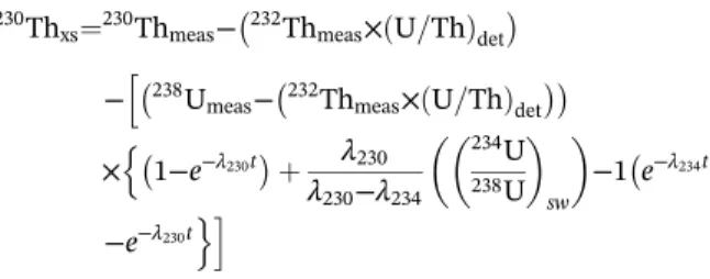
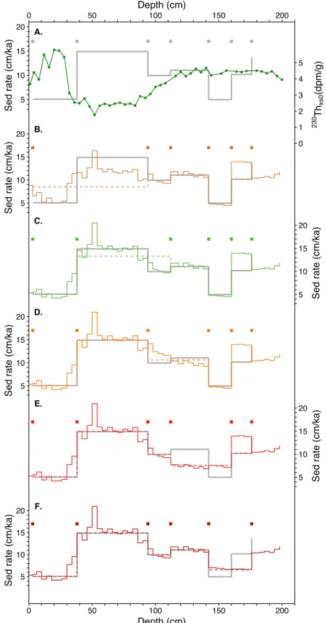
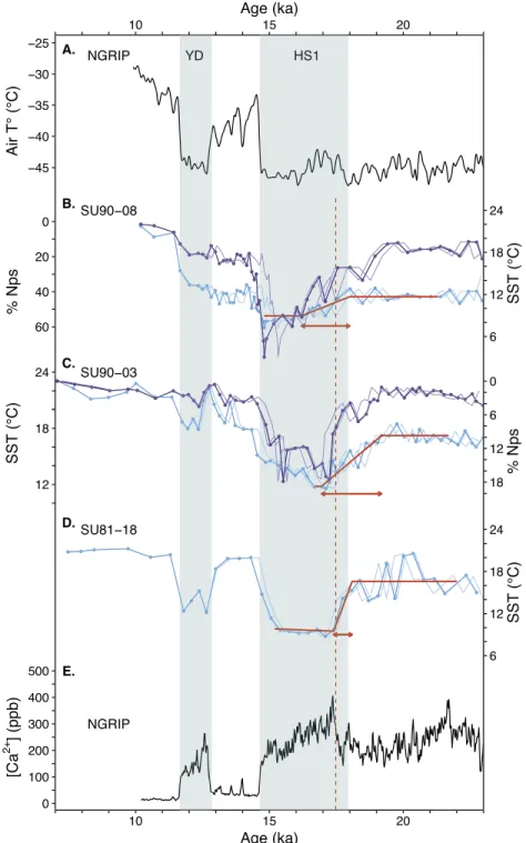
Improving North Atlantic Marine Core Chronologies Using ²³⁰Th Normalization

Recommendations can be summarised as follows: it would be important to communicate on why scientific and political considerations must be jointly taken into account to arrive

It contains the average optical depth, the control parameters (SNR* and SVCAD), the level 1 attenuated backscatter calibration relative difference between HSRL and CALIPSO,

True fossil rhopalosomatids (i.e., Eorhopalosoma gorgyra Engel, 2008; Eorhopalosoma lohrmanni Boudinot and Dungey, 2020; Rhopalosoma his- paniola Lohrmann (in Lohrmann et al.,

Abbreviations are 3pf, Three Pagodas fault; AB, Afghan block; ao, Andaman ophiolite; akms, Ayimaqin–Kunlun–Mutztag suture; assr, Andaman Sea spreading ridge; assz, Ailao Shan

We present dissolved and particulate measurements of these three thorium isotopes in a hydrothermal plume observed in the southeast Pacific Ocean on the GEOTRACES GP16 section..

In a few cases, a supersonic pulsed jet spectrum at 15 K previously obtained at lower resolution (Rostas et al. 1994 ) was used in order to disentangle the regions where the lines

The CIS method (for combing-imaging by SIMS) combines DNA combing on a silicon surface, flooding the surface with cesium, and the sensitive imaging technique of dynamic

This paper addresses the question of animal remains (isolated bones and complete skeletons) discovered in the fill of Roman sanctuary wells in northern France and their links with