HAL Id: hal-01730884
https://hal.inria.fr/hal-01730884
Submitted on 14 Mar 2018
HAL is a multi-disciplinary open access
archive for the deposit and dissemination of
sci-entific research documents, whether they are
pub-lished or not. The documents may come from
teaching and research institutions in France or
abroad, or from public or private research centers.
L’archive ouverte pluridisciplinaire HAL, est
destinée au dépôt et à la diffusion de documents
scientifiques de niveau recherche, publiés ou non,
émanant des établissements d’enseignement et de
recherche français ou étrangers, des laboratoires
publics ou privés.
Simulation and Optimization of Stall Control for an
Airfoil with a Synthetic Jet
Régis Duvigneau, Michel Visonneau
To cite this version:
Régis Duvigneau, Michel Visonneau.
Simulation and Optimization of Stall Control for an
Air-foil with a Synthetic Jet. Aerospace Science and Technology, Elsevier, 2006, 10 (4), pp.279-287.
�10.1016/j.ast.2006.01.002�. �hal-01730884�
Simulation and Optimization of Stall Control
for an Airfoil with a Synthetic Jet
Régis Duvigneau and Michel Visonneau Laboratoire de Mécanique des Fluides CNRS UMR 6598
Ecole Centrale de Nantes
B.P. 92101, rue de la Noe FR-44321 Nantes, France Michel.Visonneau@ec-nantes.fr
Abstract
This study concerns the simulation and optimization of stall control, using a synthetic jet. The flow is
simulated by solving unsteady Reynolds-averaged Navier-Stokes equations with a near-wall low-Reynolds
number turbulence closure. The flow around a NACA 0015 airfoil, including a synthetic jet located at12%
of the chord, is studied for a Reynolds numberRe = 8.96 105 and for angles of attack from 12 to 24
degrees. The optimization of the control parameters (momentum coefficient, frequency, angle w.r.t. the
wall) is intended, by coupling an automatic optimization algorithm with the flow solver. A significant
im-provement of the control efficiency is obtained (maximum lift increased of 34% and stall delayed from19◦
to22◦
w.r.t. the initial controlled flow). A Physical analysis of the flow is performed to characterize the
optimal control process found.
Keywords : Flow control, Navier-Stokes, optimization, aerodynamic stall, synthetic jet
1
Introduction
Flow control using pulsated jets has been an active topic of research for many years. Indeed, flows can
be modified by introducing jets with ad-hoc properties to obtain desired characteristics. At the present
time, most applications concern aerodynamics problems. The aerodynamic properties of an airfoil, such
as lift, drag or pitching moment, can be easily and quickly modified using flow control strategies, without
modification of the angle of attack or flap deflection[13]. Most flow control techniques are based on jet
suction and blowing. However, there are some difficulties to implement such devices into practical airfoils,
since a large amount of power and room for air supply is required. Recently, an innovative actuator, called
and its efficiency was demonstrated experimentally by several authors[13].
Some numerical investigations concerning lift increase using synthetic jets were reported in the
litter-ature, solving time-accurate Reynolds-Averaged Navier-Stokes equations. Wu et al.[14] investigated
post-stall lift enhancement for a NACA 0012 airfoil using a normal suction/blowing jet located at 2.5% of the
chord and found that lift increase in the post-stall regime can be achieved, as was reported in experiments.
The same approach was employed by Hassan et al.[8] for a slot at 13% of the chord, for different
ampli-tudes and frequencies. It was reported that a high momentum coefficient was required to obtain a significant
lift increase. Steady blowing as well as oscillatory jet actuations were simulated by Donovan et al.[3] and
compared to experimental measurements. The same configuration was also studied by Ekaterinaris[6], who
tested some different jet parameters.
All these numerical studies intend for describing the flow control process and for understanding the
connection between the actuator parameters and the control efficiency. However, a systematic search “by
hand” of the optimal control parameters is time consuming, since one time-accurate computation has to
be performed for each attempt. Therefore, the automatic optimization of the parameters of a synthetic jet
(momentum coefficient, frequency and angle w.r.t. the wall) is investigated in the present study, by coupling
an optimization algorithm with a flow solver. The numerical methods used for the simulation of the flow
are described in the first sections and applied to study the flow around a NACA 0015 airfoil including a
synthetic jet. Then, the optimization procedure is detailed and applied to determine the optimal control
parameters of the synthetic jet. Finally, a physical analysis of the flow is performed to understand why the
optimal control found is efficient.
2
Simulation of stall control
2.1
Numerical methods
The numerical simulation of stall control is performed by the ISIS flow solver, developed by EMN (Equipe
Modélisation Numérique i.e. CFD Department of the Fluid Mechanics Laboratory). The prediction of
massively separated flows, such as flows encountered in stall control, is a difficult task. Although Large
Eddy Simulation (LES) approaches may be more suitable for such flows, the present approach relies on
solving Unsteady Reynolds-averaged Navier Stokes equations (URANSE). Indeed, the computational cost
of LES approaches is still prohibitive for high Reynolds numbers, particularly in a design optimization
framework.
gen-eralized form of Gauss’ theorem): ∂ ∂t Z V ρdV + Z S ρ(−→U −−→Ud) ·−→n dS = 0 (1a) ∂ ∂t Z V ρUidV + Z S ρUi( − → U −−→Ud) ·−→n dS = Z S (τijIj−pIi) ·−→n dS + Z V ρgidV (1b)
whereV is the domain of interest, or control volume, bounded by the closed surface S moving at the
velocity−→Udwith a unit normal vector−→n directed outward.
− →
U and p represent respectively the velocity and
pressure fields. τij andgiare the components of the viscous stress tensor and the gravity, whereasIj is a
vector whose components vanished, except for the componentj which is equal to unity.
All the flow variables are stored at the geometric center of the arbitrary shaped cells. Volume and
surface integrals are evaluated according to second-order accurate approximations. Numerical fluxes are
reconstructed at the mesh faces, by using the values of the integrand extrapolated linearly from the
neigh-boring cell centers. For the diffusive terms, a centered scheme is employed, whereas a combination of
upwind and centered schemes are used for convective terms. It results from a local blending factor based
on a continuous exponential scheme involving the signed Peclet number at the face [1]. Finally, the spatial
discretization is second-order accurate.
A pressure equation is obtained in the spirit of the Rhie and Chow procedure. Momentum and pressure
equations are solved in an segregated way like in the well-known SIMPLE coupling procedure.
The temporal discretization is based on a three-step scheme, yielding a second-order accuracy:
∂A ∂t ue
cAc+ epAp+ eqAq, (2)
wherec represents the current time step, p and q the past time steps. The coefficients ec,epandeq are
chosen to ensure a second-order accuracy and depend on the steps length. All spatial terms appearing in
equations (1a) and (1b) are discretized at the current time step, yielding an implicit scheme.
Several turbulence closures are included in the flow solver, ranging from linear eddy-viscosity based
models to full second order closures [5]. For this study, the near-wall low-Reynolds number SST k − ω model of Menter is chosen, since it behaves satisfactorily for separated flows over airfoils. Turbulent
variablesk and ω are evaluated by solving transport equations which are discretized as the momentum
equation. The capability of the flow solver to accurately predict turbulent flows has been demonstrated in
2.2
Computational results
The flow control experiments of Gilarranz et al.[7] around a NACA 0015 airfoil for a Reynolds number
Re = 8.96 105 are considered as a test case. However, the purpose of this study is not to reproduce
these experiments, since they are characterized by three-dimensional and transitional effects. They are only
considered as a starting point for the optimization problem.
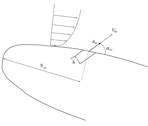
To modelize the synthetic jet actuator, a suction/blowing type boundary condition is used. Thus, a
prescribed velocity distribution is imposed at the jet boundary:
− →
U = Ujetsin(2πNjett)f (s)
− →
djet (3)
where−→djetis a vector of unit length representing the direction of the jet outlet. αjetis the angle between
− →
djet and the wall (figure 1).f (s) is the distribution of the velocity along the jet boundary. It is supposed
to have a negligible influence on the flow, as shown by Donovan et al.[3]. Therefore, a “top hat”
distribu-tion is adopted, corresponding tof (s) = 1. Concerning the turbulent variables, zero Neumann boundary
conditions are imposed on the jet boundary fork and ω.
In the experiments of Gilarranz et al.[7], the actuation is performed by a synthetic jet located atSjet=
12% of the chord L from the leading edge, with a slot width h = 0.53% of the chord (figure 2). Among
the parameters values tested experimentally, a non-dimensional frequencyNjet= NexpL/U∞= 1.29 and
a non-dimensional velocity amplitudeUjet = Uexp/U∞ = 1.37 are retained because of the satisfactory
results obtained (with U∞ the free stream velocity,Nexp the frequency of the jet andUexpthe velocity
amplitude of the jet). The jet outlet is almost tangential to the wall. Then, we impose a small angleαjet=
10◦
for the conputations. These values correspond to a momentum coefficientCµ = hUexp2 /LU 2
∞ =
0.0099.
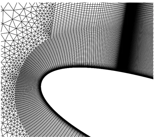
An unstructured grid including 84 577 cells is used for the calculations. This grid is composed of a fine
mesh with quadrangular cells close to the wall and in the near wake, in order to get an accurate description
of the vortex shedding, and a triangular mesh around to reduce the grid size. The distance between the first
node and the wall corresponds toy+
= 0.3. The number of nodes on the suction side of the airfoil is 364
and a refined area is located at the jet slot, which is described by 45 faces (figure 2). All computations are
performed on the same mesh.
A non-dimensional time step∆t = 5. 10−3is chosen in order that each flow cycle be described by a
sufficient number of time steps. Time-accurate calculations are initialized with uniform flow fields and are
performed until the non-dimensional timet = texpU∞/L = 70 (with texpthe physical time), for which a
periodic flow is observed.
a NACA 0015 airfoil without actuation (referred as "baseline airfoil"), and then the flow around an airfoil
including a synthetic jet with the control parameters described above (referred as "controlled airfoil with
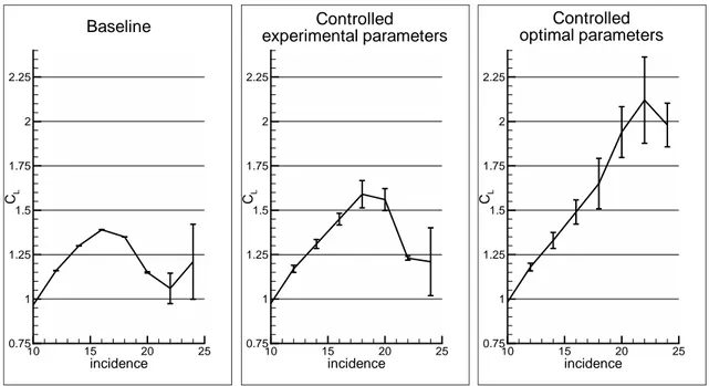
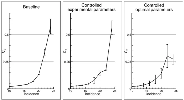
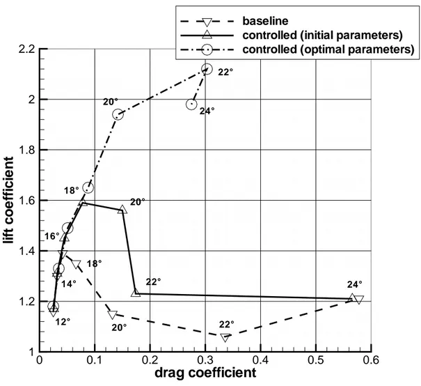
experimental parameters"). Figures 3 and 4 show the evolution of the time-averaged lift and drag
coef-ficients w.r.t. the angle of attack. On these figures, error bars represent the variations of the intantaneous
aerodynamic coefficients along time. For the baseline airfoil, the flow is rather steady until20◦
. Stall occurs
at16◦
, caused by a growing recirculation zone which appears for14◦
at the trailing edge. In the post-stall
regime, after22◦
, the flow is detached on the whole suction side of the airfoil and a counter-rotative vortices
shedding occurs, yielding a severe drag increase. For the controlled airfoil with experimental parameters,
the flow is always unsteady, due to the presence of the oscillatory jet. It generates some small vortices
which are convected downstream along the suction side of the airfoil. The actuation does not modify the
time-averaged aerodynamic coefficients until14◦
, but it maintains the lift increase until18◦
. At20◦
and
22◦
, the lift is still higher than that of the baseline airfoil, although decreasing, and the drag increase is
restrained. However, at24◦
the actuation has no more influence on the flow, which is characterized by the
same counter-rotative vortices shedding as the flow around the baseline airfoil. It yields a strong increase of
the drag and the variation of the efforts along time is growing. Finally, the comparison of the drag polar for
the baseline airfoil and the controlled airfoil with experimental parameters (figure 5) shows that the benefit
of the control is substantial, but limited from16◦
and20◦
.
3
Optimization of stall control
3.1
Methodology
Design optimization consists in maximizing an objective functionF which depends on the design variables D and the flow variables Q(D). The governing equations of the flow R(D, Q(D)) = 0 are considered as
constraints which must be satisfied at each step of the design procedure. Some bound constraints must be
added to the problem in order to find a realistic solution. Thus, the variation domain of the design variables
is usually closed. From a mathematical point of view, the problem may be expressed as:
Maximize F (D, Q(D))
Constrained to R(D, Q(D)) = 0 Li≤D ≤ Ls
In the present work, the objective function is the time-averaged lift coefficientCl(D, Q(D)) of the
during a sufficient long time to take into account several flow cycles: F (D, Q(D)) = 1 t2−t1 Z t2 t1 Cl(D, Q(D))dt (4)
In practice, the above integration is performed during about 1000 time steps. Some numerical experiments
have shown that this interval of integration is large enough in order that the time dependency be negligible.
The design variablesD are the control parameters of the synthetic jet: the velocity amplitude Ujet, the
jet frequencyNjetand the direction of the outletαjet.
Therefore, the design procedure consists in several unsteady flow simulations for a synthetic jet with
different control parameters, whose values are modified by an optimization algorithm. Thus, the design
procedure is described by :
(1) Initialization of the design variablesD
(2) Unsteady simulation of the flowQ(D)
(3) Evaluation of the time-averaged liftF (D, Q(D))
(4) Update ofD by the optimization algorithm
(5) Goto step (2)
until the convergence of the design variables is achieved. This design cycle is performed for each angle
of attack, in order to observe its influence on the optimal control parameters found.
In optimization, the use of gradient-based methods is usually motivated by their efficiency, since they
can reach a maximum of the objective function in a number of evaluations lower than zero-order methods.
However, some difficulties arise when they are faced with complicated realistic problems. The evaluation
of the derivatives of the objective function for a sophisticated simulation process is rather problematic.
Their evaluation is usually based on an adjoint formulation, which relies on the differentiation of the flow
solver [11, 9]. This task is tedious when high-order discretization schemes on unstructured grids are used,
or complex turbulence models are employed. This approach often needs an a-priori simplification of the
problem, neglecting turbulence sensitivities for instance, or using first-order discretization schemes, which
provides an approximated gradient. It has been shown by Anderson and Nielsen [11] that these
simplifi-cations often lead to erroneous gradient values. Moreover, these algorithms are very sensitive to the noisy
errors arising from the evaluation of the objective function and generating irregularities and spurious local
maxima. These sources of errors were studied by Madsen [10], who underlined the high-frequency errors
introduced by the use of high-order discretization schemes and low converged solutions. Thus, this
doubt.
To overcome these limitations, we choose to employ a derivative-free algorithm, which is easier to
implement in a complex numerical framework. It can be easily associated with a sophisticated flow solver,
since the solver is considered as a black-box and is not modified when included in the design procedure.
Furthermore, this approach is less sensitive to the noise, because no information about the derivatives is
needed to predict the optimization path. The number of evaluations required is higher than that necessited
by gradient-based methods, but it remains reasonable, as soon as the number of design variables is low,
which is the case in the present study.
The optimization method used to lead the search is based on the multi-directional search algorithm
developped by Torczon[2]. This algorithm is inspired from the Nelder-Mead simplex method, used by the
authors in the past for shape optimization purpose[4, 5].
This algorithm consists in moving a simplex ofn + 1 vertices in Rn (a triangle in R2, a tetrahedron
in R3, etc), for a problem ofn design parameters, each vertex representing a distinct design. The moves
are performed reflecting the whole simplex with respect to the best vertex, until a maximum is reached.
The simplex can eventually be expanded or contracted to adapt itself to the local topology of the objective
function.
3.2
Computational results
Between 15 and 20 optimization steps are required to reach the stopping criterion of the algorithm, for
which design variables have converged to their optimal values. It corresponds to about 45 to 60 unsteady
simulations for each angle of attack. Since it represents a large computational cost, a multi-block domain
partitioning approach is used. Actually, each optimization exercise takes about 100 hours of elapsed time
using 16 processors.
As can be seen in figure 3, the optimizer fails to significantly increase the lift as long as the flow is
fully attached. Nevertheless, between14◦
and18◦
, the control with optimal parameters provides a more
efficient actuation than that with the experimental parameters, since the slope of the lift coefficient w.r.t.
the angle of attack is slightly increased. Moreover, the actuation is efficient for higher angles of attack,
since the stall is delayed to22◦
, which corresponds to an increase of 34% of the maximum lift coefficient
w.r.t. the airfoil with experimental parameters. These results clearly show that the choice of the control
parameters is critical to obtain a large stall delay. However, the optimal control found is characterized by
a larger variation of the efforts along time for all angles of attack. The drag is similar for the two sets of
parameters from12◦
to20◦
(figure 4). At22◦
, the drag obtained for optimal parameters is characterized
24◦
, the drag using optimal parameters is far lower than that using experimental parameters. Indeed, it was
found that the experimental control has no more influence on the flow for this incidence, contrary to the
optimal control. Finally, the comparison of the drag polar (figure 5) puts in light the benefit obtained thanks
to the optimization procedure.
The optimal design parameters found are shown on table 1. Except for the incidence12◦
, for which no
significant improvement is observed, some tendancies can be drawn. First, the amplitude of the jet velocity
Ujetis increased to a mean value ofUjetopt= 1.72. The increase of the control efficiency and the enlargement
of the lift variation as the velocity amplitude grows was reported by some numerical studies [3, 6, 12] as
well as experimental observations[13]. Then, the angle between the jet outlet and the wall is increased to a
a mean value of aboutαoptjet = 25◦
. This tendency is in agreement with the computations of Ekaterinaris[6]
for trailing edge control and Donovan et al.[3] for leading edge control. The most interesting parameter
is the frequency. Indeed, except for the incidence12◦
for which no significant improvement is observed,
most optimal frequencies found are very close to each other, with a mean value ofNjetopt = 0.85. This
decrease of the frequency may also be responsible for the increase of the lift variation, as reported in the
litterature[6, 13]. Only one optimal value, at22◦
, significantly differs, since the optimal frequency found is
Njetopt22= 0.25. For this very low actuation frequency, the flow is characterized by a large vortex shedding,
which is responsible for the severe drag increase, although the lift is maintained.
A physical analysis of the flow is now performed to understand how these optimal parameters can
generate an efficient control process. The characteristics of the flow for an angle of attack of20◦
are
compared for experimental and optimal control parameters. This analysis is not performed at the incidence
22◦
, which corresponds to the maximum lift, since the very low optimal frequency found at this incidence
can be considered as doubtfull. The analysis is focused on the comparison of the lift history, the pressure
coefficient at the wall, the streamlines and the velocity profiles at different stations for experimental and
optimal control parameters.
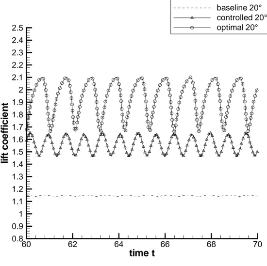
The lift history (figure 6) shows a tendency to move away from a simple sinusoidal curve. The variation
of the lift is larger, but the time-averaged lift remains higher than that with the initial parameters, at all
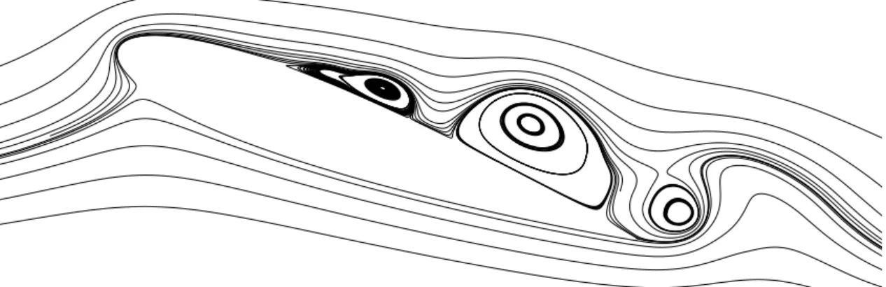
times. To understand the reasons of this higher lift, consider the streamlines on figure 7. It provides a
snapshot of the flow just at the end of suction, which corresponds to the phaseΦ = 2πNjett = 0. As
can be seen, three vortices are convected along the suction side of the airfoil for experimental parameters,
whereas only two vortices are observed for optimal parameters. This characteristic is due to the fact that
the actuation frequency is decreased. Therefore, the flow can be considered as more attached in the second
case. It provides a first explaination of the higher lift observed for the optimal parameters. The presence
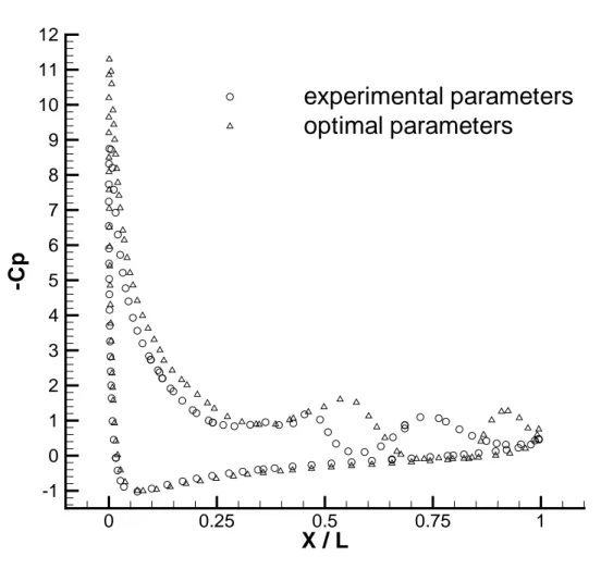
of the recirculation zones is also noticed on figure 8, which represents the pressure coefficient at the wall,
side of the airfoil. However, this figure shows that the main reason of the higher lift is due to the presence
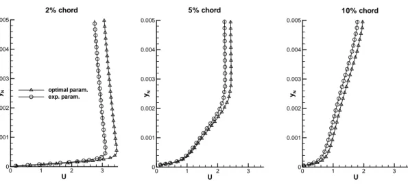
of a far higher suction peak for the optimal parameters (+31%). The velocity profiles at different stations
are computed and compared for experimental parameters and optimal parameters in figure 9. The2% chord
station corresponds to the suction peak location, whereas the10% chord station is located just upstream the
slot. As can be seen, optimal control parameters yield higher velocities in the boundary layer (about+10%)
whatever the station, which maximizes suction effects. This velocity increase is observed in the boundary
layer as well as in the outer zone, and finally vanishes as one moves away from the airfoil. In conclusion,
these comparisons show that the efficiency of the control is mainly related to the capability of the actuation
to accelerate the flow in the vicinity of the leading edge and to minimize the detachment area on the suction
side of the airfoil.
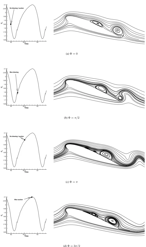
To have a better description of the flow dynamics, streamlines, velocity profiles and pressure coefficients
at different times in a cycle are represented in figures 10, 11 and 12 for the optimal parameters. The phase
Φ = 0 corresponds to the end of suction with a zero mass flow, Φ = π/2 to the maximum blowing, Φ = π
to the end of blowing with a zero mass flow andΦ = 3π/2 to the maximum suction. The streamlines
history is correlated to the lift history during a cycle (figure 10). As can be seen, a counter-rotative vortices
shedding occurs at the beginning of the blowing stage, which corresponds to the lowest lift times. Then, the
lift increases from the maximum blowing time to the maximum suction time. New vortices are generated
on the suction side at these times. Then, these vortices grow and the lift decreases as the suction is reduced.
The pressure coefficient history (figure 11) shows that the suction peak intensity is almost constant during
the whole cycle, ensuring a high time-averaged lift. Then, lift variations are due to the convection of vortices
along the suction side of the airfoil. The velocity profiles at different stations shown in figure 12, confirm
that the oscillatoring flow actuation generates variations of the velocity profiles close to the slot. Especially,
the velocity upstream of the slot is increased during the suction stage. However, the influence on the velocity
profiles far upstream is almost independent of the time, as the suction peak intensity.
4
Conclusion
The simulation of aerodynamic stall control using a synthetic jet actuator is performed, by solving
un-steady Reynolds-averaged Navier-Stokes equations, for a NACA 0015 airfoil and a Reynolds number
Re = 8.96 105. The flow solver is then coupled with an automatic optimization procedure, which relies
on a derivative-free multi-directional search algorithm. For each angle of attack, the velocity amplitude,
the frequency and the angle w.r.t. the wall are optimized to increase the time-averaged lift. Experimental
parameters are chosen as starting parameters for the optimization.
chosen. The maximum lift is increased by +34% and the stall delayed from19◦
to22◦
, w.r.t. the
experi-mental parameters. The optimal parameters are characterized by an increase of the velocity amplitude and
a decrease of the actuation frequency.
The physical analysis of the flow shows that the efficiency of the control is mainly related to the
capabil-ity of the actuation to accelerate the flow in the vicincapabil-ity of the leading edge and to minimize the detachment
area on the suction side of the airfoil.
5
Acknowledgements
The authors gratefully acknowledge the scientific committee of CINES (project dmn2050) and IDRIS
(project 1308) for the attribution of CPU time.
References
[1] I. Demirdži´c and S. Muzaferija. Numerical method for coupled fluid flow, heat transfert and stress analysis using
unstructured moving meshes with cells of arbitrary topology. Comput. meth. Appl. Mech. Eng., 125:235–255,
1995.
[2] J.E. Dennis and V. Torczon. Direct search methods on parallel machines. SIAM Journal of Optimization, 1(4):448–
474, 1991.
[3] J.F. Donovan, L.D. Kral, and A.W. Cary. Active flow control applied to an airfoil. AIAA Paper 98–0210, January
1998.
[4] R. Duvigneau and M. Visonneau. Shape optimization for incompressible and turbulent flows using the simplex
method. AIAA Paper 2001–2533, June 2001.
[5] R. Duvigneau, M. Visonneau, and G.B. Deng. On the role played by turbulence closures for hull shape
optimiza-tion at model and full scale. Journal of Marine Science and Technology, 8(1), June 2003.
[6] J.A. Ekaterinaris. Active flow control of wing separated flow. ASME FEDSM’03 Joint Fluids Engineering
Conference, Honolulu, Hawai, USA, July 6-10, 2003.
[7] J.L. Gilarranz, L.W. Traub, and O.K. Rediniotis. Characterization of a compact, high power synthetic jet actuator
for flow separation control. AIAA Paper 2002–0127, September 2002.
[8] A.A. Hassan, F.K. Straub, and Charles B.D. Effects of surface blowing/suction on the aerodynamics of helicopter
rotor blade-vortex interactions - a numerical simulation. Journal of American Helicopter Society, 42:182–194,
April 1997.
[9] A. Jameson, L. Martinelli, and N. A. Pierce. Optimum aerodynamic design using the Navier-Stokes equation.
Theorical and Computational Fluid Dynamics, 10:213–237, 1998.
[11] E. Nielsen and W. K. Anderson. Aerodynamic design optimization on unstructured meshes using the
Navier-Stockes equations. AIAA Journal, 37(11):1411–1419, 1999.
[12] S.S. Ravindran. Active control of flow separation over an airfoil. Technical Report TM-1999-209838, NASA,
1999.
[13] A. Seifert, A. Darabi, and I. Wygnanski. Delay of airfoil stall by periodic excitation. AIAA Journal, 33(4):691–
707, July 1996.
[14] J.M. Wu, X.Y. Lu, A.G. Denney, M. Fan, and J.Z. Wu. Post-stall lift enhancement on an airfoil by local unsteady
List of Figures
Fig. 1 Problem description
Fig. 2 Mesh close to the jet
Fig. 3 Lift coef. with respect to the angle of attack
Fig. 4 Drag coef. with respect to the angle of attack
Fig. 5 Drag polar
Fig. 6 Lift coef. history at20◦
Fig. 7 Comparison of the streamlines forΦ = 0
Fig. 8 Comparison of the pressure coefficients forΦ = 0, computed for experimental and optimal
parameters
Fig. 9 Comparison of the velocity profiles for Φ = 0, computed for experimental and optimal
parameters
Fig. 10Streamlines for different times
Fig. 11Pressure coefficients for different times
jet jet
h
α
S
d
jetU
jetincidence CL 10 15 20 25 0.75 1 1.25 1.5 1.75 2 2.25 Controlled optimal parameters incidence CL 10 15 20 25 0.75 1 1.25 1.5 1.75 2 2.25 Controlled experimental parameters incidence CL 10 15 20 25 0.75 1 1.25 1.5 1.75 2 2.25 Baseline
incidence CD 10 15 20 25 0 0.25 0.5 Baseline incidence CD 10 15 20 25 0 0.25 0.5 Controlled experimental parameters incidence CD 10 15 20 25 0 0.25 0.5 Controlled optimal parameters
drag coefficient
li
ft
c
o
e
ff
ic
ie
n
t
0
0.1
0.2
0.3
0.4
0.5
0.6
1
1.2
1.4
1.6
1.8
2
2.2
baseline
controlled (initial parameters)
controlled (optimal parameters)
12° 14° 16° 18° 18° 20° 20° 20° 22° 22° 22° 24° 24°
time t
li
ft
c
o
e
ff
ic
ie
n
t
60
62
64
66
68
70
0.8
0.9
1
1.1
1.2
1.3
1.4
1.5
1.6
1.7
1.8
1.9
2
2.1
2.2
2.3
2.4
2.5
baseline 20°
controlled 20°
optimal 20°
(a) Experimental parameters
(b) Optimal parameters
X / L
-C
p
0
0.25
0.5
0.75
1
-1
0
1
2
3
4
5
6
7
8
9
10
11
12
experimental parameters
optimal parameters
Figure 8: Comparison of the pressure coefficients for Φ = 0, computed for experimental and optimal
U yN 0 1 2 3 0 0.001 0.002 0.003 0.004 0.005 5% chord U yN 0 1 2 3 0 0.001 0.002 0.003 0.004 0.005 10% chord U yN 0 1 2 3 0 0.001 0.002 0.003 0.004 0.005 optimal param. exp. param. 2% chord
Time CL 62 62.5 63 1.65 1.7 1.75 1.8 1.85 1.9 1.95 2 2.05 2.1 No blowing / suction (a) Φ = 0 Time CL 62 62.5 63 1.65 1.7 1.75 1.8 1.85 1.9 1.95 2 2.05 2.1 Max blowing (b) Φ =π/2 Time CL 62 62.5 63 1.65 1.7 1.75 1.8 1.85 1.9 1.95 2 2.05 2.1 No blowing / suction (c) Φ =π Time CL 62 62.5 63 1.65 1.7 1.75 1.8 1.85 1.9 1.95 2 2.05 2.1 Max suction (d) Φ = 3π/2
X / L -C p 0 0.25 0.5 0.75 1 -1 0 1 2 3 4 5 6 7 8 9 10 11 12 Φ= 0 (a) Φ = 0 X / L -C p 0 0.25 0.5 0.75 1 -1 0 1 2 3 4 5 6 7 8 9 10 11 12 Φ=π/ 2 (b) Φ =π/2 X / L -C p 0 0.25 0.5 0.75 1 -1 0 1 2 3 4 5 6 7 8 9 10 11 12 Φ=π (c) Φ =π X / L -C p 0 0.25 0.5 0.75 1 -1 0 1 2 3 4 5 6 7 8 9 10 11 12 Φ= 3π/ 2 (d) Φ = 3π/2
U yN 0 1 2 3 0 0.001 0.002 0.003 0.004 0.005 10% chord U yN 0 1 2 3 0 0.001 0.002 0.003 0.004 0.005 5% chord U yN 1 2 3 0.001 0.002 0.003 0.004 Φ= 0 Φ=π/ 2 Φ=π Φ= 3π/ 2 2% chord
List of Tables
Ujet Njet αjet Exp. 1.37 1.29 10.00 Opt.12◦ 1.94 1.28 10.00 Opt.14◦ 1.76 0.88 30.15 Opt.16◦ 1.36 0.88 27.51 Opt.18◦ 1.76 0.88 31.25 Opt.20◦ 1.61 0.93 19.68 Opt.22◦ 1.87 0.25 35.00 Opt.24◦ 1.74 0.81 25.95