Self-consistent quasi-static radial transport during the substorm growth phase

(1)

HAL Id: hal-02550837

https://hal.archives-ouvertes.fr/hal-02550837

Submitted on 11 Jan 2021

HAL is a multi-disciplinary open access

archive for the deposit and dissemination of

sci-entific research documents, whether they are

pub-lished or not. The documents may come from

teaching and research institutions in France or

abroad, or from public or private research centers.

L’archive ouverte pluridisciplinaire HAL, est

destinée au dépôt et à la diffusion de documents

scientifiques de niveau recherche, publiés ou non,

émanant des établissements d’enseignement et de

recherche français ou étrangers, des laboratoires

publics ou privés.

Self-consistent quasi-static radial transport during the

substorm growth phase

O. Le Contel, R. Pellat, A. Roux

To cite this version:

O. Le Contel, R. Pellat, A. Roux. Self-consistent quasi-static radial transport during the substorm

growth phase. Journal of Geophysical Research Space Physics, American Geophysical Union/Wiley,

2000, 105 (A6), pp.12929-12944. �10.1029/1999JA900498�. �hal-02550837�

(2)

JOURNAL OF GEOPHYSICAL RESEARCH, VOL. 105, NO. A6, PAGES 12,929-12,944, JUNE 1, 2000

Self-consistent quasi-static radial transport

during the substorm growth phase

O. Le Contel

Centre d'Etude des Environnements Terrestre et Planetaires, Vdizy, France

R. Pellat

Centre de Physique Th•orique, Ecole Polytechnique, Palaiseau, France

A. Roux

Centre d'Etude des Environnements Terrestre et Planetaires, Vdizy, France

Abstract. We develop a self-consistent description of the slowly changing magnetic

configuration

of the near-Earth plasma

sheet (NEPS) during substorm

growth phase.

This new approach

is valid

for quasi-static

fluctuations

co

< kllv

• (v• being

the

Alfv•n velocity), with characteristic

frequency

lower than the bounce

frequencies

of

electrons

•nd ions (co

< w•i,w•,), •nd for spatial scales

l•rger th•n the ion L•rmor

radius. The basic equations are obtained from a linearization of the cyclotron and bounce-averaged Vlasov equation, together with Maxwell equations. The Vlasov- Maxwell system of equations is solved for the quasi-dipolar NEPS region. Using a 2-D dipole for the equilibrium, we calculate analytically the perturbed components of the electromagnetic field as a function of an external forcing current. The

quasi-neutrality

condition (QNC) is solved

via an expansion

in the small parameter

T,/Ti (T,/Ti is the ratio between

the electronic

and ionic temperatures). To the

lowest order in T,/Ti, we find that the enforcement

of QNC implies the presence

of

a global electrostatic potential which is constant for a given magnetic field line but varies across the magnetic field. The corresponding electric field shields the effect of the inductive component of the electric field, thereby producing a partial reduction of the motion that would correspond to the inductive electric field. Furthermore, we show that enforcing the QNC implies a field;aligned potential drop which is

computed

to the next order in T,/Ti in a companion

paper [Le Contel et al., this

issue]. In the present paper, we show that the direction of the azimuthal electric

field varies along the field line, thus the equatorial electric field cannot be mapped

onto the ionosphere.

Furthermore

during the growth phase,

the (total) azimuthal

electric field is directed eastward, close to the equator, and westward, off-equator.

Thus large equatorial pitch angle particles drift tailward, whereas small pitch angle

particles drift earthward.

1. Introduction

The process(ses) by which the plasma is transported in the Earth's magnetosphere is a critical issue, and

there is no consensus yet about its exact nature. Earlier

models are generally based on simple assumptions: a static magnetospheric electric field (i.e., an electric field derived from a scalar potential), driving a steady earth- ward "convective" motion (e.g., Cowley and Ashour-

Oa. tt.

..a

low

velocities deduced from the measurements of coherent

Paper number 1999JA900498.

0148-0227 / 00 / 1999 J A 900498 $09.00

and incoherent scatter radar tend to support the view

that there is a regular earthward convective motion no-

tably prior to substorms

[e.g., Forme et al., 1998]. In

the case of incoherent scatter radar, however, the Earth rotation is used to build maps of the flow velocity in the ionosphere, thus a steady state (over one Earth ro- tation) is implicitly assumed. However, electric field and/or flow velocity measurements, carried out in the magnetosphere on board several spacecraft, are not easy

to reconcile with the simple view of a steady convec-

tion. Huang and Frank [1986] carried out a statisti- cal survey of plasma flows, measured on ISEE 1, in- side the plasma sheet. In their survey they excluded flow velocities above 150 km/s. Their results show that

the average flow is too small to account for the rate

(3)

12,930 LE CONTEL ET AL.: SELF-CONSISTENT QUASI-STATIC RADIAL TRANSPORT

expected by steady convection models. Baumjohann

et al. [1989] conducted a survey of slow and fast flows

from AMPTE/IRM data. While slow flows were ob- served most of the time, in agreement with Huang and

Frank [1986], Baumjohann et al. [1989], taking advan-

tage of a better time resolution, gave evidence for tran-

sient bursts of fast flows, with speeds above 300 km/s, generally directed earthwards (at least inside of 19 RE being the Earth radius). Conversely, the slow flows have no preferred direction. Angelopoulos et al. [1992] further analyzed the fast flow bursts and defined bursty bulk flows (BBFs); these authors suggest that most of the radial transport of the flux could be effected through

these short lasting but intense flow bursts. These mea- surements indicate that there is not a unique regime. These results and other similar results, not described

here, have led Ifennel [1995], to introduce the possibil-

ity of a bimodal plasma sheet flow, to stress the differ- ence between the morphology of fast laminar flows and slow turbulent flows. The standard convection models, based on a constant potential electric field, do not de-

scribe these complex situations characterized either by a high temporal variability of the fast transient BBFs,

or by slow flows with no obvious preferred direction. Thus "one wonders if steady uniform convection has

ever been found" [Kennel, 1995, p. 22].

In the present paper we do not assume any static convection electric field. We adopt a different view point and investigate the transport under the influence of an externally applied electromagnetic perturbation that mimics the variation induced by the solar wind. What is the difference between a steady convection and

a time-dependent transport? In a steady state mag-

netosphere the electric field can only be electrostatic. Then, the assumption of the absence of a parallel elec-

tric field Ell is equivalent

to consider

the magnetic

field

lines

as equipotentials

(Ell = -O•/O1 -- 0 ,e--5 the po-

tential electrostatic • is independent of 1 the distance

along the magnetic field line). Conversely, in a non-

stationary

approach,

Ell:-0•/01-

O/OtAll- 0

ß +O/Ot

f dlAll

- const,

where

5All

in the parallel

com-

ponent of the vector potential. Therefore the absence of parallel electric field does not imply the equipotentiality of the magnetic field lines but only that the variation along the field line of the electrostatic component of the electric field cancels the inductive component. Thus, for a time-dependent perturbation the mapping between the equatorial and the ionospheric electric fields is not granted. Here we investigate the relation between time-dependent transport and the formation of thin cur-

rent sheets (TCS) during the substorm growth phase.

For the sake of simplicity, in the rest of the paper, we will call "convection" a steady motion driven by a con-

stant (e.g., dawn to dusk) electric field, derived from

a constant scalar potential. The term "transport" will be used to describe the effect of time varying perturba- tions, associated for instance with a growing current in

the tail.

The theoretical basis of standard convection mod- els also deserves some discussion. Most of the mod-

els rely upon the assumption

that convecting

particles

are moving in a given magnetic

field; in other words,

no attempt is made to take into account the effect the

particles have on the fields; the approach is not self-

consistent, which introduces serious limitations on the

significance

of the results.

MHD is a priori

more

appeal-

ing, because

it is self-consistent,

and provides

a simple

description

of plasma

dynamics

[Schindler

and Birn,

1982; Erickson,

1992]. The validity of the MHD ap-

proach,

however,

is also

subject

to restrictions.

Indeed,

MHD approach is only valid for perturbations whose

the frequency

is greater

than kllVe

(kll being

the par-

allel component of the wave vector and ve the thermal

velocity

of the electrons).

In a magnetic-mirror

geom-

etry as the NEPS, particles are trapped between mir- ror turning points. Therefore the validity condition of

MHD writes

w > woe

- ve/Lll (Lll being

the magnetic

field length) or equivalently the characteristic timescale

• < roe, the bounce

period of electrons.

In the NEPS,

at 7 RE, •'• is typically

1 s for energetic

electrons

(1

keV). Thus

MHD is not a valid

approximation

for long-

period fluctuations (see, for instance, Rosenbluth and

Varma

[1967],

Rutherford

and Frieman

[1968],

Anton-

sen and Lane [1980],

and Hurricane

et al. [1994]).

The

bounce

resonance

is only one of the nonlocal

processes

that limit the validity

of MHD; the magnetic

field gra-

dient, the pressure gradient, also introduce nonlocal ef-

fects,

as will be discussed

in the course

of the paper. See

also discussions on the importance of these resonances

by Chen

and

Hasegawa

[1988,

1991],

Cheng

[1982],

and

Cheng and Johnson [1999].

Plasma transport can also be achieved via low-

frequency

hydromagnetic

waves,

as discussed

by John-

son and Cheng

[1997]

and by Chen

[1999].

These

works

are based

on a quasi-linear

formalism

applied

to the gy-

rokinetic

equations;

hence

the rate of transport

is pro-

portional

to the square

of the amplitude

of these

hydro-

magnetic waves. Observations carried out in the near-

Earth plasma sheet (NEPS), for instance, by GEOS-2

[Roux

et al., 1991],

show

that during

the growth

phase,

the amplitude

of hydromagnetic

waves

is very weak.

Thus wave-induced

transport

is unlikely

to play an im-

portant role during the growth phase. While periodic

oscillations are negligible, one regularly observes a slow change in the magnetic configuration that will be mod-

eled as a quasi-static

perturbation.

Therefore,

in the

present

paper we describe

a linear selLconsistent

ap-

proach

to the transport

of the plasma

in the NEPS,

in response

to quasi-static

variations

of the magnetic

field. We use an approach

developed

for electromag-

netic perturbations with a frequency lower than the

bounce

frequency

of electrons

and ions

(w < woi,wo•)

and for spatial scales larger than the ion Larmor ra-

dius (kñp < 1), but we neglect

Alfv•n waves,

assum-

ing w < kllV

A. The present

approach

is based

on the

linearized

response

of the plasma

to low frequency

dec-

(4)

LE CONTEL ET AL.: SELF-CONSISTENT QUASI-STATIC RADIAL TRANSPORT 12,931

tromagnetic perturbation (w < w0) obtained by Pellat

from the Vlasov equation by assuming conservation of

the first adiabatic invariant [Pellat, 1990]. The response

of the plasma is completed by Maxwell equations. For

long perpendicular wavelength electromagnetic pertur-

bations

(k_cAD

<< 1, where

/•D- V/eokBT/(noq

2) is

the Debye length, e0 is the vacuum permittivity, kB the Bolztmann constant, T the temperature, no the den-

sity, and q the charge of particles), the Gauss's equation

reduces to the QNC. Yet, owing to the low frequency of the perturbations, we need to take into account the existence of nonlocal terms. For instance, in the elec- trostatic case, for a multipole, the QNC implies the ex- istence of an electrostatic perturbed potential (I'0 con-

stant along the field line [Pellat et al., 1994]. This result

has been extended to electromagnetic perturbations by

Hurricane et al. [1995b] for w > w.,•d (w, being the diamagnetic drift frequency and •d being the bounce- averaged magnetic drift frequency), and applied to the

magnetotail. In section 2.2 we solve the QNC to the

lowest order in T,/Ti < 1 and give a generalization of

Hurricane 's result valid for perturbations with arbitrary frequencies.

Finally, the system is completed by the parallel and p,•rpendicular projections of the AmpSre's law. Unlike substorm injection which is known to be a sudden pro-

cess

(w >_ wt>i)

with a small spatial scale (ky --> c•),

the buildup of a tail-like configuration is a slow process

(•_ 30 rain) affecting

a large fraction

of the tail (small

ky). Thus the applied

electromagnetic

perturbation

is

not considered as being the consequence of a local inter-

nal instability (as it is probably the case for breakup).

The change from a dipole to a tail-like configuration, in- stead, is considered as the result of the response of the

magnetotail to a quasi-static forcing caused by varia- tions in the solar wind [e.g., Jacquey, 1996]. The full

treatment of this problem is very difficult since it would

require a full description of the forcing caused by the so- lar wind, taking into account the boundary conditions

imposed at the magnetopause. Moreover, the way the solar wind drives the stretching of the magnetic field lines is still not completely understood. To simplify, we assume that the change of the dipolar field close to the

Earth is due to an increase of the westward current far-

ther in the tail [e.g., Jacquey, 1996], neglecting the local electrical currents (low/3 assumption, /3 being the ra-

tio between the kinetic pressure and the magnetic pres-

sure). Thus, for the equilibrium,

Amp•re's law gives

• x • - -•. Perturbing

the

equilibrium

with

an

exter-

nal current

located

far from

the dipqlar

re, on,

we

solve

the

linearized

Amp•re's

law

gives

• x 5t{ = luoS-•ext

to obtain the perturbed components of the magnetic

field.

The above few lines suggest the following questions,

to be discussed in the course of the paper: (1) What

are the consequences of enforcing the QNC in a time-

dependent situation? (2) What is the role of the time

varying

electric

fields (associated

with electromagnetic

perturbations) on the transport of the plasma inside the plasma sheet? (3) Can we map the electric field from

the equatorial magnetosphere, down to the ionosphere during the growth phase?

The linearized response of the plasma is described in subsection 2.1 and the QNC is solved in subsection 2.2. In subsection 2.3 we build a Green function and solve the linearized Amp•re's equation to obtain the perturbed magnetic field from the external current. In order to allow an analytical approach, a simple mag-

netic field model, a two-dimensional (2-D) dipole, is

used. This model is also presented in subsection 2.3. In section 3 we give the spatial profile of the azimuthal electric field along the field line and show the implica- tions on the transport of the plasma across magnetic field lines during the growth phase. The solution of the

QNC, to the first order in (Te/Ti), will be described in a companion paper [Le Contel et al., this issue], to-

gether with its consequences, namely the development of a finite parallel electric field.

2. Linearized Vlasov-Maxwell

System of

Equations

2.1. Solution of the Bounce-Averaged Vlasov Equation

Assuming that the electromagnetic perturbation is

periodic in time (t) and in space (across the magnetic

field)

we take

the_Derturbing

electrostatic

(5(•) and

magnetic vector (5.4) potentials as

5•( r-•,

t), 5--•(•,

t)

-- •'•(•,

cv,

l),

•(•, w,

l)exp

[i(•. • + wt)],

where

• (•)is the position

vector

(the

wave

vec-

tor) and ß denotes the component perpendicular to the

magnetic field. For the sake of simplicity we omit the hat symbol and the exponential factor in the following formulas, then the linearized response 5f is given by

5 f - q• 5• - u•SA•

+ (1

+ •)Ae

-is-

(1

+ •)g], (1)

where fo(E, py) is the equilibrium distribution function (E is the particle energy and py the canonical momen-

tum), uy is the diamagnetic

drift velocity,

w• = ky'uy

is

the diamagnetic drift frequency, ky is the wavenumber in the y direction (azimuthal). We work in local field-

aligned coordinates defined by the triad of unit vectors:

In this frame, the velocity becomes

(5)

12,932 LE CONTEL ET AL' SELF-CONSISTENT QUASI-STATIC RADIAL TRANSPORT

To obtain the linear response (1), a change of vari-

ables

(v½, %, vii

) --• (E, p, •) has been

made,

where

•mVll

q-/•B is the kinetic

energy,

/• •mv_c

is the magnetic moment, and • is the gyrophase angle.

The elementary

volume

in velocity

space

becomes

dav=

•o--x,+x Bd•d•d•/("•21v,

l), where

cr- sign(vii

) (for

more details, see Rutherford and Frieman [1968], Hur-

ricane [1994],

and Hurricane

eta!. [1995a,

b]). In (1)

the function g contains the nonlocal wave-particle inter- action. To first order in w/coo, the function g becomes

-is

• •

+ (rico

I-•111

H-

co+cod J

,

(4)

S-

k_cv_c

sin(ak- •)/i2, ak - Arctan(k½/ku),

i2 is

the cyclotron frequency, cod - kuvd is the gradient-

curvature drift frequency, the upper bar denotes bounce averaging and H is given by

(o:

+ o:•)

,X

H - Jo (•4> - vddAy) +

(5)

where

,k - ico

ft dl/JoSAl[

and

,h, are

Bessel

functions

of argument kzlvz[/l•. In the next section we sub-

stitute the linearized solution of the Vlasov equation into the QNC. The bounce-averaged linear solution of Vlasov equation obtained here is similar to those devel-

oped and used by different authors [e.g., Antonsen and Lane, 1980; Uheng, 1982; Chen and ttasegawa, 1991].

2.2. Quasi-neutrality Equation

In this subsection, we solve the QNC via an expansion in the small parameter T•/Ti. The validity of this ex- pansion is suggested by several observations indicating that this ratio is small in the magnetotail. For instance,

Lui et al. [1992] presented a statistical study of cur-

rent disruptions from AMPTE/CCE when the space- craft was in the near-Earth current sheer. They showed that the electron to proton [emperature ratio is in [h.e range of 0.11 to 0.57. They poin[ed out that these val- ues are higher than those reported by Baumjohann et al.

[1989] based on IRM data. Indeed, Baumjohann et al. [1989] obtained average plasma properties, notably an

electron to proton [emperature ratio in the range: 0.09- 0.18. These authors also noticed that this ratio is nearly

the same as the one found by Slavin et al. [1965] a[ distances of 1x1:30-60 P,E. More recently, during a

dusk-dawn crossing of the near-Ear[h tail by Geotail, during a relatively quiet period, a ratio around 0.2 was

measured [Frank et al., 1996]. It is therefore possible to consider T•/T/as a small parameter over a wide range of

radial distances from the Earth, and for different levels of a.ctivity.

From the linear response of the plasma (equations (1)

to (5)) and assuming

that f0 is a Maxwellian

distribu-

tion

function

(fo -no [m/(2•rT)]a/2xp-(E/T)),

the

QNC'

Ej=i,e

qj f d3 5 fj __•

0 can

be written

i • q

J 1 4

•r

B

d

E

d

/u

**(• +•* •+•*•'i•o]**

+ & • O, (6)

where we have performed the gyrophase integration and summed over streaming and antistreaming velocities. This latter operation cancels out the part of 5f that is

an odd function of rr. The above relation was derived earlier by Hurricane ½t al. [1995b], where more details are given about the derivation. The gauge SAy = 0

has been chosen. Since we are interested in large-scale

perturbations (the growth phase), the usual wavelength ordering k_cpj << i is made. In this limit, the Bessel functions become J0 -• 1 and J• •_ k_clv_cl/2i2, and the

expression for H simplifies; we get

H - 54> + • + • (7) where E - codA/co- ilukydA½/q. Then, after some alge-

braic manipulations, the QNC can be written as

• -•" (• + x) - • + •" (•)

(8) where the terms co.j,X cancel between electrons and ions, because ttyi/• } q- ttye/Te -- O, [Hurricane et al.,

1995b]. Note that the diamagnetic drift frequency and the purely magnetic drift frequency of electrons can easily be related to the corresponding terms for ions:

-t6

- -•/•/T/

(where

cod•(oz)

-- -T•/• •')(•) and •.•

•.i

th means thermal quantities and • denotes the particle

pitch angle). The QNC becomes

f 4•BdEd•

_{•'•;•i fo•}

_{(• - •) + (• - x)}

+ • ((• -•)+ (x- •))

: •

m7lvlll

foi •(•

- ]

+ •.,- •, (•) . (•)

Since the right-hand side (RHS) term of (9) is propor-

(6)

LE CONTEL ET AL.' SELF-CONSISTENT QUASI-STATIC RADIAL TRANSPORT 12,933

J 4rcBdEdl•

+ - X)]

- 0

+

A •rivial solution of (10) is + - y) +

where •0 is constant for a given magnetic field line. This constant component of the perturbed electrostatic

potential is always taken to be equal to zero (5•+h - 0) in studies based on MHD. An external electrostatic

field, modeling the convection, is often added to the inductive part of the electric field in order to better fit

the data [e.g., Sauvaud et al., 1996]. In the present pa-

per, we show that the quasi-neutrality over the volume of the flux tube implies that •0 is different from zero. We compute •0 in a self:consistent manner, as a func- tion of the electromagnetic perturbation defined by h

and 5Bii. Integrating

the QNC (9) over the volume

of

the flux tube, we find

m7lvl

fog

(• + 7•i ) • + 7•i '

where the left-hand side (LHS) term of (9) has vanished

thanks

to the identity

f dl/B f dav(X - •) - O, valid

for any function X(E, •, l). Finally, •0 writes

f f

0iL

ß 0 =

[,

[

]'

f •

4••

**foi •"•(•*•-•"•**

(13)

Now, we can calculate the self-consistent perturbed electric field. Taking in•o account the implications of

•he QNC (11) [o the lowest order in T•/Ti,. [he per-

ubed daic

i.

y direction, becomes (remembering •ha• $Av - 0)'

-

Thus the complete perpendicular electric field associ- ated with the perturbation is the sum of an inductive

component

(,•) plus an electrostatic

component

((I>0)

de-

termined from the QNC. This electric field will produce a transport of the plasma. Notice that this transport is different from a steady convection; it is associated

with an electromagnetic perturbation (see discussion in introduction). The electrostatic component, associated

with •0, tends to reduce the effect of the inductive com-

ponent of the electric field ,•, thereby producing a par-

tial shielding of the motion that would correspond to

the inductive electric field (if it was not shielded). This

effect can explain why large bulk flows are not detected in the NEPS during the growth phase.

The

expression

I - iw

ft dl•dAll

shows

that

the

par-

tial derivative of I with respect to 1 is equal to the in-

ductive component of the parallel electric field (Ol/Ol =

05All/Or

). Thus locally

and in the limit Te < Ti, (11)

implies that the inductive component of the parallel

electric

field OdAll/Ot

is balanced

by the parallel

gra-

dient of the perturbed electrostatic potential Odq)/Ol. Hence (11) is equivalent to the usual MHD approxima-

tion, where one assumes the absence of a parallel electric

field (Ell: -0/0l(5• + A) = 0). In the present

study,

the absence of a parallel electric field is not an assump-

tion but an (approximate) result, obtained by solving

the QNC in the limit Te < iF/. We show, however, in a

companion paper [L½ Contel et al., this issue], that the solution of the QNC to the first order in (T•/T/) allows

us to compute a finite parallel electric field.

Studying low-frequency perturbations, Chcn and

Hasegawa [1991] considered a magnetospheric plasma consisting of two populations: a core (100 eV) and an energetic component (10 keV). In their work the core

population is denser than the energetic population and therefore plays a key role in the QNC. For this popu- lation, 0:b• > 0: > wbi. They obtained d• + l = 0, i.e.,

no parallel

electric

field (dEll : -0t(d(I)+ A) - 0). In

the present work carried out for 0:•,0:•i > 0:, we also

find dell •- 0 in the limit T• < T/ since

we have ob-

tained &I) + l: (I)0(g', y) where 4)o is constant along a

field line. However, this constant potential (I)0 modifies the perpendicular transport of tile plasma as already

mentioned.

Finally, one should notice that the perpendicular elec-

tric field (14) varies along the field line even when there

is no parallel electric field. Thus, in the quasi-static limit, the absence of a parallel electric field does not im- ply that the equatorial perpendicular electric field can be mapped onto tile ionospheric electric field. This is

true only in the purely electrostatic case (steady convec- tion); an assumption which is certainly not valid during

the growth phase. In the next subsectiOn, we solve the Ampare's law to determine the magnetic field pertur-

bation.

2.3. Ampare's Law

Close to the Earth, we can neglect the local elec-

trical currents which corresponds to assuming/7 < 1. Thus we can approximate the field by a dipole. To al-

low us to carry out analytical calculations, we use a

two-dimensional (2-D) dipole [Huang and Birmingham,

1994]

to describe

the equilibrium

magnetic

field. Using

cylindrical coordinates (r,O,y) where 0 is the colatitude,

the 2-D magnetic field model is defined by

/) (cos

Ou-?

+ sin

Ou---•),

(15)

where

• is the dipolar

moment.

The magnetic

field

(7)

12,934 _{LE CONTEL ET AL.' SELF-CONSISTENT}_QUASI-STATIC_{RADIAL TRANSPORT}

B- Beq

sin

2 0'

(16)

where

Beq

-- iS/L

2, is the equatorial

magnetic

field

strength, L is the equatorial-crossing distance of the relevant field line. For the 2-D dipole the local coordi- nates become

½- -15/L,y,x- bcotO/L.

(17)

It follows

that

•- X• x e-•y,

and

the

magnetic

field

strength is

B-

;)2

_(•8)

/• sin

2 [arccot

(-X/O)]

The bounce

period and the bounce

average

curvature-

gradient magnetic drift velocity are

2rrL / dl -2E

rt, -

• -

--v-'•

- •

e-•. (19)

v '

vii

qLBeq

Then, we perturb

the dipolar

equilibrium

by an external

current, flowing in the westward direction and located

far in the tail. The linearized AmpSre's law becomes

• x • - luo5j•te-•y.

(20)

We assume that

5---•(-½r

, t) -- •(O, ky,

l, w)

exp

[i(kyy

+ wt)],

for the sake of simplicity

we omit the hat symbol

and

the exponential

factor in the following

formulas. The

external current 5j•t is defined by

5j•t(L, ky, O,

co): (Sjeq(ky,

co)(5(L

- Lc)

ß

sin

"•0[(2n+l)cot

20-1]. (21)

We have assumed that the current is highly localized in radial distance, and we choose for simplicity a Dirac function 5(L-Lc), where Lc is the radial location of the

forcing current. Therefore we are interested in L values

between

0 < L < L• where

the 2-D dipole

assumption

is

valid. Along the field line, we have chosen a class of forc- ing current whose the dependence allows us to obtain

easily

the magnetic

field perturbation

and corresponds

to an increase

in the equatorial

current

as suggested

by the observations

[e.g.,

Sauvaud

and Winckler,

1980;

Scrgecv

et al., 1993]. This class

is labeled

by an index

n, the larger n, the more localized

is the perturbation

close

to the magnetic

equator

(see

Figure

1). Compari-

son

between

results

obtained

for various

n gives

insight

on how sensitive

the results

are to the 0 dependence

of

the forcing

current. For n = 0 the perturbed

current

is divergent at high latitudes but as we will check later

on, this divergence

does

not modify the results

because

the perturbed

components

of the electromagnetic

field

do not diverge.

For the sake

of simplicity,

in the course

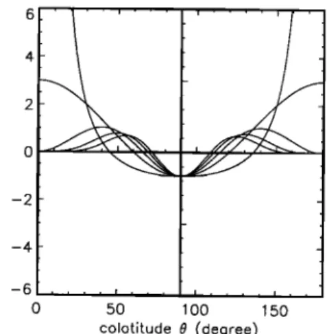
6 4 2 0 -2 -4 -6 0 50 100 150 colotitude 0 (degree)

Figure

1. Variation

of the external

current

(Sjyezt(O)

OC

sin

2"

0 ((2n

+ 1)cot

2 0- 1) versus

the colatitude

0 for

n - 0, 1, 2, 3, 4.

of the paper, we often use the case n - 0 to obtain

estimates

of the various

characteristic

quantities.

After

some

algebra

(described

in Appendix

A) and,

in

the limit Iky[L

> 1 and Iky(L- Lc)l < 1, the perturbed

components of the magnetic field write

5B½ - -

..olkvlaj•q(k

v.

w) (sin

2r•+1

0 cos

O)

2 '

For A, we obtain

(Appendix

A)

(22)

(23)

A..(L.

kv.O.w

) - A,•q

[c•(L.

kv)

q- (sin

2 0)•+1],

(24)

where

we

have

defined

c•(L,

ky)- (n +

L•)[)

•+1 and

A•,q

-- 1/[4(n+

1)]po([kv[/kv)•dj•q(kv,•)

ß

L•L.To

obtain

the real

components

of •he perturbed

magnetic field, we have •o perform an inverse Fourier

tra,nsform

in time

and

in y. We

find

(see

Appendix

B)

-

coO)

5j•q(y'.?

Pf(l•dy'(::;;•-) (25)

2 L

- (2n

+ 2)sin2

0]

{H(L-

L•)

- H[-(L-

L•)]}

(26)

Now, we have to specify the variation of the current in

(8)

LE CONTEL ET AL.' SELF-CONSISTENT QUASI-STATIC RADIAL TRANSPORT 12,935

servations close to midnight [McPhemvn, 1979; Sauvaud and Winckler, 1980; Roux et al., 1991] show that the

magnetic field changes from a dipole-like configuration

to a tail-like configuration. The equatorial value of the magnetic field decreases, whereas, off-equator, the ra- dial component increases. The duration of this vari- ation is typically •_ 30-45 min. Moreover, breakup is usually observed to start close to midnight in a longitu- dinally narrow sector, while the rest of the magnetotail keeps on stretching [Nagai, 1991]. These observations

suggest

that while the reconfiguration

at breakup

is lo-

calized in longitude, the formation of the current sheet during the growth phase is more homogeneous in lon-

gitude. Thus, while the limit ky -+ cxv

is adapted

to

study breakup, the formation of the current sheet can be better described by a finite ky. Therefore we consider

an external current localized around the noon-midnight

meridian, flowing eastward and slowly increasing with

the time as

y2

5jeq(y,

t) -- 5j,•

exp(-•¾)exp('/t),

(27)

where

5jr• is the initial magnitude

of the current, 1/7

is the characteristic time scale of the growth phase, and A is the characteristic scale along y where the tail cur- rent increases. The complete expression of the external

current becomes

5je•t(L, y, O,

t) - 5j•q(y, t)5(L - L•)

ß

sin

2n

t9

[(2n

+ 1)cot

2 0 -- 1].

(28) We verify that for 19 : rr/2 (magnetic equator), the forcing current flows westward as suggested by observa- tions. Then, we can compute the •) component of the

perturbed magnetic field which gives

5B½ =

ttodj,•

_ Lc

2 (sin2,,+z

0cos

0)

V'•

ß

(29)

where

I•V(C)

- 1/(x/•) f-•o dV exp(-V2)/(V-()is the

Fried-Conte function and we have defined 1/ - y•/A and • - y/A. Close to midnight, • < 1, and in this limit, the Fried-Conte function can be approximated

by Pf(r7V(•'))

"• -2• + O(• a) and

we obtain

yo6j.•

_{Vff Lo}

2 (sin2,•+•

₀

_cos

O)

]

ß

]-- 1-2(X)

A

2 ß

(30)

One should notice that in the opposite limit ( > 1 (far

away

of the lnaxm•um

of the current

in the y direction),

the expansion

of the Fried-Conte

function

is -1/( and

5B• = 0. Finally,

close

to lnidnight

(( < 1), the two

perturbed components of the magnetic field write

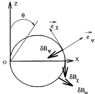
O Z

5B

x

Figure 2. Schematic diagram of the electromagnetic perturbation applied on a 2-D dipole field to model the change of configuration which occurs during the growth phase. As indicated by the arrows, the magnetic field perturbation tends to produce a tail-like configuration.

5B½: Po6j,•

_{• L•}

2 (sin2,•+•

_0cos

O)

ß

511--

05q(V, 0 + 1)

2 L

- (2n

+ 2)

sin2

01{H(L-

L•)

-H[-(L-L•)]}.

(32)

We verify that for a forcing current directed westward

(5j,• > 0) at the magnetic

equator (19: rr/2), the ra-

dial component of the equilibrium magnetic field in- creases off-equator, whereas the equatorial component decreases, which corresponds to observations carried

out during the growth phase (see Figure 2).

3. Transport of the Plasma

In the previous subsections 2.1, 2.2, and 2.3, we have V, asov-Maxwell system of equa- completely solved the

tions

in the quasi-static

limit, (w < kllVA

and

In (5), only the terms

w•/w and it•kySA

½/q - -SB[/q

appear. It is useful to compare the size of these two

terms. Remembering

that w•tA/w •_ ky¾•,Aneq/CO

and

1•8Bil/q

-- -t•B}>/q •' E[-2(n u,_

l):•,•q]/•/b/q

1/(kyL)ky7•A•q/W, we c•.•t conclude

that, in the limit

IklL >

we have t•6BiI/• < waA/w. Thus the term

containing

dBii can be neglected.

In this case

the lin-

earized Vlasov equation, which describes the behavior

(9)

12,936 LE CONTEL ET AL' SELF-CONSISTENT QUASI-STATIC RADIAL TRANSPORT

the same but the expression (5) of H becomes Then, in the limit • < 1 we obtain

+ )

H - J05(I>

+

A ,

(33)

5Ey - 5Eœ,y,t(L,

y, t)

where 5(I) is given by the QNC (9) that implies 5(I) =

(I)0- A, with (I)0 given

by (13), and A and 5Bii given

by

(24) and (32) (from the Ampare's law solved in the limit

> 1

< 1). Now, obtain

the self-

consistent perpendicular electric field associated with the magnetic field perturbations, we need to compute the constant part, (I)0, of the perturbed electrostatic

potential.

Taking

into account

that/USBll/q

the expression, (13), of (I)0 becomes

l [s,•

- (sin2

0)

'•+1]

n+l

(41)

where we have defined

5E•:

_,,

y t(L

_,,

y t) - _/•odj,•7L•L

₂

1 'X

X

exp(7t). (42)

The colatitude 0 where the perpendicular electric field changes sign is given by

f •_.

{f 4•rBdEd/•

.•fl•,l fo•

(34) From the expression (24) of • we obtain (see Appendix C)

1 I

u

Beq

E

1 + k

lu

Beq

E (35)

Then, we compute the expression of (I)0 (see Appendix

D) and obtain

'I'o- (c• + S•)A.•q, (36)

where we have defined

(37) Now, from (14), the self-consistent perpendicular elec- tric field writes

00 - arcsin

(S,•w•+•)

.

(43)

Because S,• is always smaller than unity, the direc- tion of the perpendicular electric field changes along the field line even in the absence of a parallel elec-

tric field (see Figure 3). As noted in section 2.2,

5Ey is directed

eastward

(positive)

close

to the equa-

tor, it is null for 0 = 00, and it is directed west-

ward (negative) for 0 < •0. The larger n, the larger is •0 therefore the region where 5Ey is eastward gets thinner (as n increases). As an example, for n = 0,

S0: 5/6, A0 = (c0

+ sin

2 e) A0•q,

•0: (c0

+ 5/6)A0•q,

and 6Ey : 6E•(L, y,t) (5/6 - sin

2 0). The elec[ric

field •Es is directed eas[ward (positive) close •o the

equa[or,

iC is null for 0 = arcsin(5/6)

1/2 and is directed

westward

(negative)

for e < arcsin(5/6)

•/• From

(42)

we can estimate the intensity of the perpendicular elec- tric field during the growth phase. For instance, the characteristic variation of the equatorial magnetic field

a[ the geostationary orbk (L• 2 L = 6.6 R•) is of order

of 30 nT for a duration of the growth phase of 30 min.

We assume thaC the radial scale of the current sheet is

m 1R•; therefore

**t*o•J• • 30 x 10-9/(6.4 x 10•)T/m.**

In the • direction we assume [hat [he spatial scale A is • 4R•. We ob[ain for the inductive component of

the perpendicular elec[ric field (without the conCribu-

5Ey

-- -ikyAneq

[Sn

-- (sin

2

(38)

After an inverse Fourier transform, we obtain

(39) 'raking into account the expression of the current (27), we find 5E'y = (40) 1.0 0.5 0.0 -0.5 -1.0 0 Ey(8) _ 50 1 O0 150 colotitude •?(degres)

Figure 3. Variation

of A and

5Ey versus

the colatitude

(10)

LE CONTEL ET AL.: SELF-CONSISTENT QUASI-STATIC RADIAL TRANSPORT 12,937

tion of (I>0),

5•'L,y,t 'm'_

2.5 mV/m which is reduced

to

0.4 mV/m at the equator due to the contribution of the electrostatic component (I>0 (S, in (41)). As we have

previously mentioned, the effect of the (I>0 is to decrease the magnitude of the total electric field compa,red to the inductive component. Therefore the plasm.• transport

is also reduced.

Next, we can compute the bounce average electric drift to study the motion of the particles along • as a function of their pitch angle. We obtain (see Appendix

__

n Ivll

i / dl

I B

5Ey

_ 5E•,u,t(L,

Beq n + 1

y,

t) 1

"+•

(2k- 1)•

-

k=0

. •(_1)•C• pB•q . (44)

E

j=0

We note that the bounce average electric drift, associ-

ated with 5Eu, depends on the magnetic moment. TO

simplify, we can consider two extreme cases: equatorial

pitch angle particles of 900 (pBeq/E • 1) and equa- torial pitch angle particles of 0 ø (pB•q/E 2 0). We

obtain

p,,+2

5EL,u,t/Beq S•/2-•u=0(-1

• ), - 0

o,

• .Ch+,(2•-

1)•/(•)• •

5EL,y,t/Beq(Sn- 1), •eq-- 900

,

where

5EL,y,t,

given

by (42) is always

negative

close

to

the midnight meridian (y < A). Since S, is always

smaller than unity the bounce average electric drift of

900 particles and that of 0 ø particles have opposite di-

rections. The 900 particles drift tailward, whereas 0 ø

particles drift earthward, during the magnetic field line

stretching. When n increases, the perturbation is more and more localized close to the equator and S, de-

creases. Therefore, from (45) we deduce that 900 parti-

cles drift more and more tailward, whereas 0 ø particles remain almost at rest. Again for n = 0, we find

1/24(5E•,u,t(L,

y,

t)/Beq),

Geq

: 0

90 ø,

o.

Thus the correct treatment of the QNC implies a per- pendicular motion in response to a quasi-static elec-

trornagnet,

ic perturbation

(w < kl!VA

and

•%t, because the perpendicular electric field direction varies with the positicr). :xlong the field line, the bounce- averaged motion is dii[•rent for different pitch angles. Ninety degrees pitch angle particles, which mirror close to tb.e equator drift tailward while zero degree parti-

cles ,•:'•ft e•rthward. This result is very different h'om

the results of Huang and t)•rmingham [1994], who con-

sider a static magnetic field and impose an electrostatic field to ensure the convection of the plasma toward the Earth. In the present work, the transport is due to the response of the plasma to the quasi-static perturbation and to the necessity of enforcing the quasi-neutrality.

4. Conclusion

In the present paper, we have given a self-consistent description of the quasi-static transport of the plasma, during the growth phase, in response to an external forcing. The full linearized Vlasov-Maxwell system of equations has been solved for quasi-static electromag-

netic perturbations,

satisfying

0: < kllvn and 0: < 0:s. In

order to get a simple equilibrium the pressure gradient

has been assumed to be small. Thus the local current is

small, and the local perturbation of the magnetic field is due to currents flowing farther in the tail. From Am- p•re's law we have obtained the perturbed components of the electric and magnetic fields as functions of the external forcing current. For the sake of simplicity, this current is assumed to be localized close to the mag- netic equator and around the noon-midnight meridian. It flows in the east-west direction, as expected during the growth phase. Using a 2-D dipole model to describe

the region close to the Earth (the NEPS), we have built a Green function to relate the fields in the NEPS with

this external driving current. Thus the solutions for the fields, in the plasma sheet, have been obtained as the products of the Green function by the forcing current. Using the linear bounce-averaged solution of the Vlasov equation obtained by P½llat [1990], the QNC has been

solved. To the lowest order in T•/• (T•/• < 1), we

found the following:

1. The QNC imposes the existence of a component

•0, given by (13), of the perturbed electrostatic po-

tential. This component •0 is constant along the field line and varies in the azimuthal direction, thereby con- tributing to the azimuthal electric field. This electric field tends to reduce the effect of the inductive compo- nent of the electric field, which explains why no large bulk flows are associated with large timescale electro-

magnetic perturbation (r > rb) like the growth phase.

Unlike what is done for the particle test and MHD ap- proaches, in the present paper, the electrostatic compo- nent of the azimuthal electric field is not assumed; it is determined, in a self-consistent manner, by the response of the plasma and related to an externally applied elec- tromagnetic perturbation. ¾Ve point out that the ex- istence of the component (I)0 is a purely kinetic effect occuring for co < co•. In a forthcoming paper we will show that the component (I)0 exists as long as co < In all cases it cannot be described by MHD.

2. The total azimuthal electric field (14), which is

the sum of these two components, varies in amplitude and direction, as a function of the position along the

(11)

12,938 LE CONTEL ET AL.' SELF-CONSISTENT QUASI-STATIC RADIAL TRANSPORT

field line. The changes in amplitude and in direction of the azinmthal electric field implies a bounce-averaged

transport of the particles (44) that strongly depends on

the pitch angle.

3. The parallel electric field is null to the order

Te/• < 1 (see (11)), therefore the residual parallel elec-

tric field should be calculated from the QNC developed

to the order Te/Ti. This calculation is presented in a

companion paper.

Notice that the full Vlasov-Maxwell system of equa- tions has been solved only in the quasi-static limit, no-

tably the solutions of Ampare's law, (31) and (32), are

valid only in this limit. However, the results obtained

to the lowest order in Te/Ti from the QNC (summa- rized above) are, also basically valid for low-frequency

perturbations co < cob. Furthermore, for the sake of sim- plicity and because in the NEPS the effect of magnetic drift. are expected to be more important than the finite larmor radius effects, the present calculations have been performed in the long wave length limit. However, we can easily include these effects if necessary since they are retained in the expression of the perturbed distri-

bution function (5).

For the magnetic field variations corresponding to the

growth phase, namely for a slow decrease (increase) of

the component of the magnetic field, perpendicular to

the equatorial plane (radial), the azimuthal electric field

is explicitly computed. It is found to be directed east- ward, close to the equator and westward off-equator.

As a consequence, during the growth phase, large equa-

torial pitch angle particles, which mirror near the equa-

tor, drift tailward, whereas small equatorial pitch angle

particles, which mirror far away from the equator, drift earthward. Furthermore, this result suggests that the mapping between the perpendicular electric field in the equatorial region and the electric field in the ionosphere

where J is the Jacobian of the change of coordinates

between the cartesian and the local frame (see also the Appendix A of Hurricane et al. [1995b]). We assume that

•---•(•r

, t) - 5--•(½,

kv,l,

co)

exp[i(kvy

+cot)],

for the sake of simplicity we omit the hat symbol and the exponential factor in the following formulas. Defining

two variables

X - ky•/co and Y - ikySAo/B as Bern-

ste•n et al. [1958], interchanging the partial derivatives,

O•(JBOt) - JBOtO•, (see Hurricane

et al. [1995b]

for

details about the interchange of the partial derivatives)

when necessary, the Amp•re's law writes

is not simple;

a self-consistent

approach,

including

non- One

can

show

that (A4) can

be obtained

from

(A2) and

local kinetic effects associated with the bounce motions (A3); therefore the system is reduced to these two latter

of particles,

is needed

to sort out the consequences

of a equations.

Inserting

(A2) to (A3), we obtain

time-dependent transport. The corresponding charac- teristic azimuthal electric field is of order of 0.4 mV/m

at the magnetic equator. In order to test these theoret- ical results it would be necessary to have electric field

and/or plasma flow data organized as a function of the distance from the center of the current sheet, during the

growth phase.

Appendix A' Solution of the Linearized

Ampre's

Law

Using the local field-aligned coordinates and with the

gauge

aA

v = 0, the

curl

of • gives

-• x '•

'• -' • •

O

y J

B

O

x • •

0½

(A5)

Again,

we interchange

the partial

derivatives

(O½(JBOt)

: JBOtO•), divide by B and integrate

along

the field

line which yields

(A6)

Therefore we hav'e to solve the following system of equa-

(12)

LE CONTEL ET AL.' SELF-CONSISTENT QUASI-STATIC RADIAL TRANSPORT 12,939

~ i 0 (0• 02X)

ki•_B

O1 '-•

aloe ' (A7)

(AS)

To go

further,

we

assume

a priori

that

O•"/O1

< 02X/O1

0• (and will check

it afterwards)

which

corresponds

to

assume

that the variation

of 5Bll along

the field line is

smaller than the variation of 5B½ in the radial direction. This assumption is well adapted to the choice of an external current highly localized in the radial direction.

The system becomes

10X

k• a• • a•a½

'

1 o B

• 0½

oto½

j.

:/-to •(•jyext

.

(A10)

Defining

a new variable,

U- ax/az, (A10) becomes

02U

_{0 In JB 20U kv}

₂

B••,

(10dB)]

I•okv2/dl

(All)

Assuming

that the perturbation

varies

faster

in the • di-

rection

than the equilibrium,

the second

term of (All)

can be neglected.

Moreover,

in the limit Ikyl

œ > 1 the

term between

parenthesis

is equivalent

to unity. There-

fore

(All) can

be rewritten

in a classical

form

of a linear

second-order differential equation: 02U 2

ky

U- S(•

B 2 ' (A12)

where

S(½,

k v, l, w) - -(luokuU/B)

f[dl/BSj•t(½,

kv,

l,

w)] is the forcing

tern,. To solve

(A12), we have

to

build a Green functie• l-kom the solutions of the ho-

mogeneous

equation;

U• - exp

(1•1 f d½/•) and

U2 -

' ,se• e.g Zwillinger, 1989]. Taking into account the properties of the 2-D dipole model it

is more convenient to use the variables L and 0 defined

by (17). While L and 0 are not strictly

speaking

inde-

pendent

variables,

we can consider

them as such

in the

-

•2L

sin

2 0 f d0sin

20dje.rt(L

where

S(L, ky, O,

w) poky

,

0, o:). Now, the solutions

of the homogeneous

equation

becorne

U1 - exp

[ky]L

sin

2 0 and

U2 - exp-Ik•,lL

sin

2 0.

The Green function is defined by

Ui(L)U2(Lo) W(Lo)

exp([ky[(L-Lo)sin29)

--

W(L0)

,0 <_

L _<

L0;

Ui(Lo)U2(L) W(Lo)

_ exp(-[kul(L--Lo)

sin

•0) Lo

• L • oo

-- W(Lo) ....

where

W(Lo) - -2lkul•in

2 o, is the Wronskian

of U1

and U2. The Green function becomes

exp

(--la•(• - •0)1

sin2

O)

2lkyl

sin

2 0

_(A14)

The complete solution of (A13) writes (omitting to specify all the dependences)