HAL Id: hal-01206707
https://hal.archives-ouvertes.fr/hal-01206707
Submitted on 29 Sep 2015
HAL is a multi-disciplinary open access
archive for the deposit and dissemination of
sci-entific research documents, whether they are
pub-lished or not. The documents may come from
teaching and research institutions in France or
abroad, or from public or private research centers.
L’archive ouverte pluridisciplinaire HAL, est
destinée au dépôt et à la diffusion de documents
scientifiques de niveau recherche, publiés ou non,
émanant des établissements d’enseignement et de
recherche français ou étrangers, des laboratoires
publics ou privés.
Stéphanie Jehan-Besson, Ariane Herbulot, Michel Barlaud, Gilles Aubert
To cite this version:
Stéphanie Jehan-Besson, Ariane Herbulot, Michel Barlaud, Gilles Aubert. Shape Gradient for Image
and Video Segmentation. Paragios Nikos, Chen Yunmei, Faugeras, Olivier. Handbook of
Mathemat-ical Models in Computer Vision, Springer US, pp.309-323, 2006, 978-0-387-28831-4.
�10.1007/0-387-28831-7_19�. �hal-01206707�
Printer: Opaque this
Shape Gradient for Image and
Video Segmentation
S. Jehan-Besson, A. Herbulot, M. Barlaud,
G. Aubert
ABSTRACT In this chapter, we propose to concentrate on the research of an optimal domain with regards to a global criterion including region and boundary functionals. A local shape minimizer is obtained through the evo-lution of a deformable domain in the direction of the shape gradient. Shape derivation tools, coming from shape optimization theory, allow us to easily differentiate region and boundary functionals. We more particularly focus on region functionals involving region-dependent features that are globally attached to the region. A general framework is proposed and illustrated by many examples involving functions of parametric or non parametric prob-ability density functions (pdfs) of image features. Among these functions, we notably study the minimization of information measures such as the entropy for the segmentation of homogeneous regions or the minimization of the distance between pdfs for tracking or matching regions of interest. Keywords: active contours, active regions, region functionals, boundary functionals, shape optimization, shape gradient, segmentation, tracking, Image statistics, non parametric statistics, parzen window, entropy, dis-tance between pdfs.
1
Introduction
Active contours are powerful tools for image and video segmentation or tracking. They can be formulated in the framework of variational methods. The basic principle is to construct a PDE (Partial Differential Equation) from an energy criterion, including usually both region and boundary func-tionals. This PDE changes the shape of the current curve according to some velocity field which can be thought of as a descent direction of the energy criterion. Given a closed curve enclosing an initial region, one then com-putes the solution of this PDE for this initial condition. The corresponding family of curves decreases the energy criterion and converges toward a (lo-cal) minimum of the criterion hopefully corresponding to the objects to be segmented.
Originally, snakes [26], balloons [8] or geodesic active contours [3] are driven towards the edges of an image through the minimization of a bound-ary integral of features depending on edges. Active contours driven by the
minimization of region functionals in addition to boundary functionals have appeared later. Introduced by [9] and [34], they have been further developed in [37, 5, 7, 32, 31, 14, 36]. Actually, the use of active contours for the op-timization of a criterion including both region and boundary functionals appears to be powerful.
However, the PDE computation is not trivial when the energy criterion involves region functionals. This is mostly due to the fact that the set of image regions does not have a structure of vector space, preventing us to use in a straightforward fashion gradient descent methods. To circumvent this problem, we propose to take benefit of shape derivation principles de-veloped by [35, 15]. This computation becomes more involved when global information about regions is present in the energy criterion, the so-called region-dependent case. It happens when statistical features of a region such as, for example, the mean or the variance of the intensity, are involved in the minimization. In this chapter, we propose a general framework based on shape derivation tools for the computation of the related evolution equa-tion. Inside this theoretical framework, many descriptors based on paramet-ric or non parametparamet-ric pdfs of image features may be studied. We propose to give some results for both of them and some examples of applications.
Region and boundary functionals are presented in section 2 while shape derivation tools are presented in section 3. Statistical region-dependent descriptors based on parametric and non parametric probability density functions (pdfs) are studied in section 4.
2
Problem Statement
In many image processing problems, the issue is to find a set of image regions that minimize a given error criterion. The basic idea of active con-tours is to compute a Partial Differential Equation (PDE) that will drive the boundary of an initial region towards a local minimum of the error criterion. The key point is to compute the velocity vector at each point of the boundary at each time instant.
To fix ideas, in the two-dimensional case, the evolving boundary, or active
contour, is modeled by a parametric curve Γ(s, τ ) = (x1(s, τ ), x2(s, τ )),
where s may be its arc-length and τ is an evolution parameter. The active contour is then driven by the following PDE:
Γτ
def
= ∂Γ
∂τ = v with Γ(τ = 0) = Γ0,
where Γ0 is an initial curve defined by the user and v the velocity vector
of Γ(s, τ ). This velocity is the unknown that must be differentiated from an error criterion so that the solution Γ(., τ ) converges towards a curve achieving a local minimum and thus, hopefully, towards the boundary of the object to be segmented, as τ → ∞.
Following the pioneer work of Mumford Shah [30], a segmentation prob-lem may be formulated through the minimization of a criterion including
both region and boundary functionals. Let U be a class of domains of Rn,
and Ω an element of U of boundary ∂Ω. A boundary functional, Jb, may
be expressed as a boundary integral of some scalar function kb of image
features:
Jb(∂Ω) =
Z
∂Ω
kb(x, ∂Ω) da(x) (1.1)
where ∂Ω is the boundary of the region and da its area element.
The most classical example of boundary functional comes from the work of Caselles et al [3], where the authors minimize for an image in 2D:
J(∂Ω) = Z
∂Ω
g(|∇I(∂Ω(s))|)ds
where s represents the arc length of the curve ∂Ω and g(r) = 1+r1m, m = 1
or 2. The function g drives the curve towards the image edges characterized by high values of the image gradient.
A region functional, J, may be expressed as an integral, in a domain Ω of U, of some function k of some region features:
J(Ω) =
Z
Ω
k(x, Ω)dx (1.2)
Let us note that the scalar function k in (1.2) is generally region-dependent. A classical example of region-dependent descriptor is the following one proposed by [5, 14]:
k(x, Ω) = (I(x) − µ(Ω))2
where µ(Ω) represents the mean of the intensity values within the region Ω. This dependency on the region must be taken into account when searching for a local minimum of the functional.
Generally one uses a linear combination of region-based and contour-based terms in order to perform a segmentation task. A simple example is
the segmentation into two regions Ωinand Ωout, which basically correspond
to objects and background. An appropriate energy functional for this task would be: J(Ωin,Ωout) = Z Ωin kin(x, Ωin) dx + Z Ωout kout(x, Ωout) dx + Z ∂Ωin kb(x) ds
where kin is the descriptor for the object region, kout for the background
region and kb the descriptor for the contour.
The choice of the descriptors is dependent on the application. In this article we propose to focus on statistical descriptors based on paramet-ric or non parametparamet-ric pdfs. Once this choice is made the terms have to be derived in order to calculate a velocity function that drives an initial
contour towards a minimum. A detailed state of the art on region-based active contours can be found in [24]. Let us briefly note that some authors do not compute the theoretical expression of the velocity field but choose a deformation of the curve that will make the criterion decrease [4, 7]. Other authors [37, 31] compute the theoretical expression of the velocity vector from the Euler-Lagrange equations. The computation is performed in two main steps. First, region integrals representing region functionals are transformed into boundary integrals using the Green-Riemann theo-rem. Secondly, the corresponding Euler-Lagrange equations are derived, and used to define a dynamic scheme in order to make evolve the initial region. Another alternative is to keep the region formulation to compute the gradient of the energy criterion with respect to the region instead of reducing region integrals to boundary integrals. In [14], the authors pro-pose to compute the derivative of the criterion while taking into account the discontinuities across the contour. In [23, 24] the computation of the evolution equation is achieved through shape derivation principles.
This computation becomes more difficult for region-dependent descrip-tors. It happens when statistical features of a region such as, for example, the mean or the variance of the intensity, are involved in the minimization. This case has been studied in [5, 14, 36, 28, 13]. In [23, 24] the authors show that the minimization of functionals involving region-dependent fea-tures can induce additional terms in the evolution equation of the active contour that are important in practice. These additional terms are easily computed thanks to shape derivation tools.
In the following, we present shape derivation tools for the computation of the evolution equation.
3
From shape derivation tools towards
region-based active contours models
As far as the derivation is concerned, two main difficulties must be solved.
First, the set of image regions, i.e. the set of regular open domains in Rn,
denoted by U, does not have a structure of vector space, preventing us from using in a straightforward fashion gradient descent methods. To circumvent this problem, shape derivation methods [35, 15] can be brought to bear on
the problem as detailed in this section. Secondly, the descriptors kr or kb
may be region or boundary-dependent. Such a dependence must be taken into account in the derivation of the functionals as pointed out in [23, 24, 1, 17]. We here recall a theorem giving relation between derivatives that will be helpful for derivation of region functionals for both region-independent and region-dependent descriptors. We also give some details and references for the derivation of boundary-based terms using shape derivation tools.
3.1
Shape derivation tools
3.1.1 Introduction of transformations
As it has already been pointed out, the optimization of the region functional
J(Ω) is difficult since U does not have the structure of a vector space.
Variations of a domain must then be defined in some way. Let us consider
a reference domain Ω ∈ U and the set ˆA of applications T : Ω → Rn, which
are at least as regular as homeomorphisms (i.e. one to one with T and T−1
continuous). We define ˆ A =©T one to one, T, T−1 ∈ W1,∞(Ω, Rn)ª where: Wn,∞(Ω, Rn) = {T : Ω → Rn such that T ∈ L∞(Ω, Rn) and ∂iT ∈ L∞(Ω, Rn), i = 1, · · · , n}
Given a shape function F : U → R+, for T ∈ ˆA, let us define ˆF(T ) =
F(T (Ω)). The key point is that W1,∞(Ω, Rn) is a Banach space. This allows
us to define the notion of derivative with respect to the domain Ω as follows:
DEFINITION 1 F is Gˆateaux differentiable with respect to Ω if and only
if ˆF is Gˆateaux differentiable with respect to T .
In order to compute Gˆateaux derivatives with respect to T we introduce a
family of deformation (T (τ ))τ≥0 such that T (τ ) ∈ ˆA for τ ≥ 0, T (0) = Id,
and T (.) ∈ C1([0, A]; W1,∞(Ω, Rn), A > 0.
For a point x ∈ Ω, we denote:
x(τ ) = T (τ, x) with T(0, x) = x
Ω(τ ) = T (τ, Ω) with T(0, Ω) = Ω
Let us now define the velocity vector field V corresponding to T (τ ) as
V(τ, x) = ∂T
∂τ(τ, x) ∀x ∈ Ω ∀τ ≥ 0
3.1.2 Relations between the derivatives
We now introduce two main definitions:
DEFINITION 2 The Gˆateaux derivative of J(Ω) =R
Ωf(x, Ω)dx in the
direction of V, noted dJr(Ω, V), is equal to:
dJr(Ω, V) = lim
τ→0
J(Ω(τ )) − J(Ω)
τ This derivative is called the Eulerian derivative.
DEFINITION 3 The shape derivative of k(x, Ω), noted ks(x, Ω, V ), is equal to: ks(x, Ω, V) = lim τ→0 k(x, Ω(τ )) − k(x, Ω) τ
The following theorem gives a relation between the Eulerian derivative and the shape derivative for the region functional (1.2). The proof can be found in [35, 15], an elementary one is provided in [24] for completeness.
THEOREM 1 The Eulerian derivative of the functional J(Ω) =R
Ωk(x, Ω) dx
in the direction of V is the following:
dJr(Ω, V) = Z Ω ks(x, Ω, V)dx − Z ∂Ω k(x, Ω)(V(x) · N(x))da(x)
where N is the unit inward normal to ∂Ω and da its area element.
Note that Theorem 1 provides a necessary condition for a domain ˆΩ to
be an extremum of J(Ω): Z ˆ Ω ks(x, ˆΩ, V)dx − Z ∂ ˆΩ k(x, ˆΩ)(V(x) · N(x)) da(x) = 0 ∀V.
3.2
Derivation of boundary-based terms
In the case of boundary-independent descriptors, the Eulerian derivative of
Jb=R∂Ωkb(x)da(x) in the direction vn= (V · N) is the following:
dJb(∂Ω, vn) =
Z
∂Ω(∇k
b(x) · N − kb(x) κ)(V · N)da (1.3)
where κ is the mean curvature of ∂Ω.
From this Eulerian derivative, we can deduce the following evolution equation for the active contour:
Γτ= (kb(x) κ − ∇kb(x) · N)N with Γ(τ = 0) = Γ0. (1.4)
This evolution equation has been computed by Caselles et al [3] by using techniques of calculus of variations.
As far as boundary-dependent descriptors are concerned, the dependence on the boundary must be taken into account for the computation of the Eulerian derivative. In [17], the authors studied the following descriptor which represents the distance between the current boundary ∂Ω and a
reference one ∂Ωref:
kb = d(∂Ω, ∂Ωref).
The authors compute the evolution equation and they show that some terms appear coming from the dependency of the descriptor with the bound-ary. This descriptor has been used for the introduction of shape prior for
segmentation. Let us note that the introduction of shape priors for segmen-tation using active contours has also been studied by [33, 11, 12]. Let us also note that in [22], the authors remind some theorems for the computa-tion of the Eulerian derivative of boundary-dependent descriptors and in [6], the authors deal with shape metrics following considerations developed in [15].
3.3
Derivation of region-based terms
Let us now apply the previous results to differentiate the velocity vector of the active contour.
3.3.1 Region-independent descriptors
We first consider the simple case where the function k does not depend on
Ω, i.e. k = k(x). In that case, the shape derivative ks is equal to zero and
the Eulerian derivative of J is simply (Theorem 1):
dJr(Ω, V) = −
Z
∂Ω
k(x)(V(x) · N(x))da(x)
This leads to the following evolution equation for region-independent de-scriptors:
Γτ = kN with Γ(τ = 0) = Γ0.
This is the classical result [37, 31] when k has no region dependency. Let us now consider the more general case where the function k has some region dependency.
3.3.2 Region-dependent descriptors
Region-dependent descriptors of the form Jr(Ω) =RΩk(x, Ω)dx are more
complicated to differentiate. Using Theorem 1 one can obtains a derivative of the following form [24, 1] for some of them (see section 4):
dJr(Ω, V) = −
Z
∂Ω¡k(x, Ω) + A(x, Ω)¢(V · N) da
(1.5) This leads to the following evolution equation for these region-dependent descriptors:
Γτ= (k + A)N with Γ(τ = 0) = Γ0.
The term A(x, Ω) is a term that comes from the region-dependence and
so from the evaluation of the shape derivative ks. We here propose a
parametric or non parametric statistics. The principle is to model region-dependent descriptors as follows:
J(Ω) = Z Ω k(x, G(Ω)) dx, where G(Ω) = Z Ω H(x, Ω) dx (1.6)
As shown in this equation, the function H is itself region-dependent, more precisely:
H(x, Ω)def= H(x, K(Ω)) , and K(Ω) =
Z
Ω
L(x) dx (1.7)
Note that we have stopped the process at the second level but it could con-ceivably continue. We have chosen this special case of dependency because it often arises in applications, as shown in sections 4.2 and 4.1.
THEOREM 2 The Eulerian derivative in the direction of V of the func-tional J defined in (1.9) is:
drJ(Ω, V) = − Z ∂Ω(A(x, Ω) + k(x, Ω)) (V(x) · N(x))da(x) where : A(x, Ω) = µZ Ω kG(x, G(Ω)) dx ¶ µ L(x) Z Ω HK(x, K(Ω)) dx + H(x, K(Ω)) 
The terms kGand HK denote respectively the partial derivative of the
func-tion k and H with respect to their second argument. Proof: According to Theorem 1, we have:
drJ(Ω, V) = Z Ω ksdx − Z ∂Ω k(V · N)da(x)
Let us first compute the shape derivative of k. From the chain rule we get:
ks(x, Ω, V) = kG(x, G)drG(Ω, V), (1.8)
where kG denotes the partial derivative of the function k with respect to
its second argument.
Next we compute the Eulerian derivative of G in the direction of V. We apply again Theorem 1, and we get:
drG(Ω, V) = Z Ω Hsdx − Z ∂Ω H (V · N)da(x).
Plugging this into (1.8), we obtain: Z Ω ksdx = µZ Ω kG(x, G(Ω)) dx ¶ µZ Ω Hsdx − Z ∂Ω H(V · N)da(x) ¶ ,
We also compute the shape derivative of H thanks to Theorem 1:
Hs(x, Ω, V) = HK(x, K)drK(Ω, V)
The Eulerian derivative of K in the direction of V is given by:
drK(Ω, V) = Z Ω Lsdx − Z ∂Ω L(x)(V (x) · N(x))da(x)
Since L does not depend on Ω, we obtain Ls= 0 and we get the result.
We can now state the result for the general case where k is described as a linear combination or region functionals as follows:
J(Ω) =
Z
Ω
k(x, G1(Ω), G2(Ω), .., Gm(Ω)) dx, (1.9)
where the functionals Gi are given by Gi(Ω) =
R
ΩHi(x, Ω) dx i= 1..m.
As shown in this equation, the function Hi is itself region-dependent, more
precisely: Hi(x, Ω) def = Hi(x, Ki1(Ω), Ki2(Ω), .., Kili(Ω)) (1.10) where Kij(Ω) = Z Ω Lij(x) dx j= 1..li i= 1..m. (1.11)
We have chosen this special case of dependency because it often arises in applications, as shown in sections 4.2 and 4.1.
THEOREM 3 The Eulerian derivative in the direction of V of the func-tional J defined in (1.9) is:
drJ(Ω, V) = − Z ∂Ω(A(x, Ω) + k(x, Ω)) (V · N)da. where A(x, Ω) =Pm i=1DiPlj=1i (BijLij(x)) +Pmi=1(DiHi), and Di = Z Ω kGi(x, G1(Ω), .., Gm(Ω)) dx i= 1..m Bij = Z Ω HiKij(x, Ki1(Ω), .., Kili(Ω)) dx i= 1..m j= 1..li
4
Segmentation using Statistical Region-dependent
descriptors
In this section, we are interested in the minimization of the region functional (1.2) for region-dependent descriptors. The general framework introduced
in section 3.3.2 allows us to compute the derivative and the evolution equa-tion for many descriptors based on parametric or non parametric statistics. Some examples of computation are given for descriptors based on paramet-ric statistics in section 4.1, while a general computation of the derivative is proposed for non parametric statistics in section 4.2.
Let us first introduce some notations and some examples of region-dependent descriptors. We note f (x) the feature of interest of the image at location x. This feature may be the intensity of the image, the motion
vector, a shape descriptor and is a function f : Ωf → Rmwhere Ωf ⊂ R2is
the image domain and m is the dimension of the feature. If f is the image intensity, m = 1 for grayscale images and m = 3 for color images. If f is a motion vector, m = 2.
When considering the pdf of f within the region, denoted by q(f (x), Ω), we can choose the following general descriptor for segmentation:
k(x, Ω) = ϕ(q(f (x), Ω)) (1.12)
When minimizing the -log-likelihood function for independent and identi-cally distributed observations (iid) f (x), we have:
ϕ(q(f (x), Ω)) = − ln(q(f(x), Ω) (1.13)
When minimizing the entropy function, we get:
ϕ(q(f (x), Ω)) = −q(f(x), Ω) ln(q(f(x), Ω) (1.14)
The concept entropy designates the average quantity of information car-ried out by a feature [10]. Intuitively the entropy represents some kind of diversity of a given feature.
These descriptors may be chosen to characterize the homogeneity of a region according to the feature. In both cases, the pdf may be parametric, i.e. it follows a prespecified law (Gaussian, Rayleigh ...) or non parametric. In the last case, no assumption are made on the underlying distribution.
As far as parametric pdfs are concerned, the descriptor (1.13) has first been introduced by [37] for the segmentation of homogeneous regions using region-based active contours and further developed by [31, 29]. In the case of parametric pdfs, the probability density function q is indexed by one or more parameters, denoted by a vector θ, describing the distribution model. For example, when using a one dimensional Gaussian distribution, we get:
qθ(f (x), Ω)) = 1 √ 2πσexp −(f(x) − µ)2 2σ2
where θ = [µ σ]T. The term µ and σ represent respectively the mean and the
variance of the scalar feature f within the region Ω. Note that the param-eters of the distribution depend on Ω and that such a dependence must be taken into account during the derivation process. Some other descriptors for
segmentation are derived from the development of the expression (1.13) for
Gaussian distributions. For example, the descriptor k(x, Ω) = (I(x) − µ)2
has been proposed by [5] for the segmentation of homogeneous regions, and
the descriptor k(x, Ω) = %(σ2) by [24].
As far as non parametric pdfs are concerned, the expression of the pdf q is given by the Parzen method [16]:
q(f (x), Ω) = 1
|Ω| Z
Ω
K(f (x) − f(ˆx)) dˆx (1.15)
where K is the Gaussian kernel of the estimation with 0-mean and σ-variance and |Ω| the shape area. Non parametric pdfs have been introduced in region-based active contours in [1] for the minimization of the distance between two pdfs and in [28] for the minimization of information measures. The general descriptor (1.12) has been studied in [20, 21] and the descriptor (1.13) has been studied by [28, 27, 2].
4.1
Examples of Descriptors based on parametric statistics
In the case of parametric pdfs, the probability density function q is in-dexed by one or more parameters, denoted by a vector θ, describing the distribution model. The parameters θ depend on the domain Ω and such a dependence must be taken into account in the derivation process through the evaluation of the domain derivative. We propose here to give some results for the derivation of functions depending on simple statistical pa-rameters such as the mean or the variance. This study can be extended to the derivation of the covariance matrix determinant.
4.1.1 Region-dependent descriptors using the mean
For a one-dimensional image feature f , let us choose:
k(x, Ω) = %(f (x) − µ) = %(f(x) − 1
|Ω| Z
Ω
f(x) dx) (1.16)
where % : R → R+is a positive function of class C1. The region functional
can be expressed as in equation (1.9): J(Ω) = Z Ω k(x, Ω) dx = Z Ω %(f (x) − µ) dx = Z Ω %(f (x) −G1(Ω) G2(Ω) ) dx, where G1(Ω) = Z Ω H1(x, Ω) dx = Z Ω f(x) dx and G2(Ω) = Z Ω H2(x, Ω) dx = Z Ω 1dx
In this case, the functions Hi, i = 1, 2 do not depend on the region Ω,
computed: D1 = −RΩG1 2 % 0³f(x) −G1 G2 ´ dx = −1 |Ω| R Ω% 0(f − µ)dx D2 = RΩ(GG1 2)2 % 0³f(x) −G1 G2 ´ dx = |Ω|µ R Ω% 0(f − µ)dx
The terms Bijare equal to zero and the velocity vector of the active contour
is then: Γτ = · k−(f − µ) |Ω| Z Ω %0(f − µ)dx ¸ N
In this example, the term coming from the region dependency of f is equal to (f −µ)|Ω| R
Ω%0(f − µ)dx. Note that in the particular case of %(r) = r2, this
term is equal to zero [5, 14].
4.1.2 Region-dependent descriptors based on the variance
Let us take another example of descriptor for one dimensional image fea-ture. Consider the case where the function k is a function of the variance given by: k(x, Ω) = %(σ2) = % µ 1 |Ω| Z Ω(f (x) − µ) 2 ¶ = %µ G1(Ω) G2(Ω) ¶ where % : R+→ R+ is of class C1.
We can then compute the velocity vector of the active contour from Theorem 3 using: G1(Ω) = Z Ω H1(x, Ω) dx , H1(x, Ω) = µ f(x) −K11 K12 ¶2 , l1= 2, G2(Ω) = Z Ω H2(x, Ω) dx , H2(x, Ω) = 1, l2= 0 , and we find: Γτ=£k + %0(σ2)¡(f − µ)2− σ2¢¤ N.
In this simple example, we notice that the dependency of the function on
the region induces the term A(x, Ω) = %0(σ2)¡(f(x) − µ)2− σ2¢
in the evolution equation, see [24] for details.
This result can be extended to a descriptor based on the covariance
ma-trix determinant for multidimensional image features f = [f1, f2, ..., fn]T.
It can be a useful tool for the segmentation of homogeneous regions since minimizing the entropy is equivalent to minimize the determinant of the co-variance matrix in the case of Gaussian distributions [19, 18]. The evolution equation can be computed using Theorem 3. Details of the computation as well as experimental results for the segmentation of the face in color video sequences may be found in [24] .
4.2
Descriptors based on non parametric statistics
4.2.1 Region-dependent descriptors based on non parametric pdfs of
image features
We consider the following descriptor, where ϕ is a function: R+→ R+ and
qis given by (1.15):
k(x, Ω) = ϕ¡q(f(x), Ω)¢ (1.17)
THEOREM 4 The Eulerian derivative in the direction V of the
func-tional J(Ω) =R
Ωk(x, Ω)dx where k is defined in (1.17) is:
dJr(Ω, V) = − Z ∂Ω¡k(x, Ω) + A(x, Ω)¢(V · N) da(x) where A(x, Ω) = − 1 |Ω| ·Z Ω ϕ0(q(f (ˆx), Ω))[q(f (ˆx), Ω) − K(f(ˆx) − f(x))]dˆx ¸
Proof: The criterion is differentiated using the methodology developed in section 3.3.2. We have: J(Ω) = Z Ω ϕ¡ G1(x, Ω) G2(Ω) ¢ dx = Z Ω f(G1(x, Ω), G2(Ω))dx with G1(x, Ω) = Z Ω H1(x, ˆx, Ω) dˆx , H1(x, ˆx, Ω) = K(f (x) − f(ˆx)), G2(Ω) = Z Ω H2(ˆx, Ω) dˆx , H2(ˆx, Ω) = 1 ,
These results can then be used for segmentation using information mea-sures such as the entropy or the mutual information [20, 21]. If we choose to minimize the entropy as in [20], ϕ(q) = −q ln(q). In Figure 1, an ex-ample of segmentation of an osteoporosis image is given by minimizing
J(Ωin,Ωout) = E(Ωin) + E(Ωout) + λRΓdswhere E(Ωin) and E(Ωout)
rep-resent respectively the entropy of the one-dimensional feature f (x) = I(x)
inside and outside the curve and λR
Γdsis the classical regularization term
that minimizes the curve length balanced with a positive parameter λ. The Figure 1 shows the evolution of the segmentation and the evolution of the
associated histograms (of the region Ωin and Ωout) during iterations.
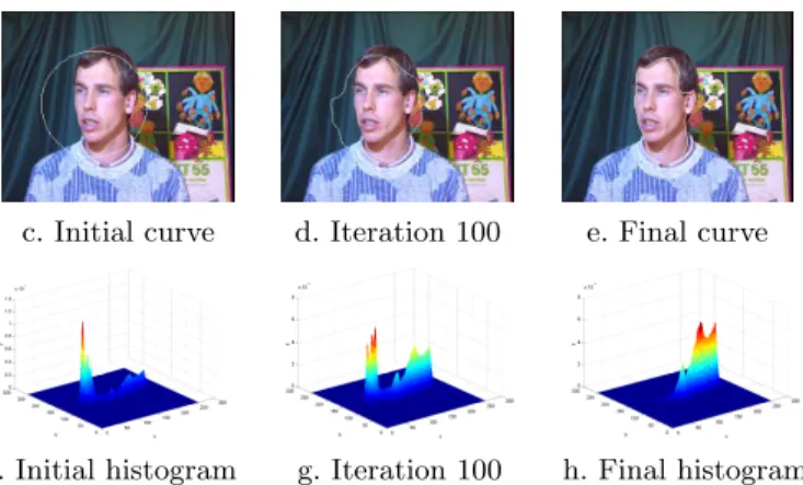
Fig-ure 2 shows an example of segmentation of color video by minimizing the
joint entropy of a two dimensional feature f (x) = [Y (x), U (x)]T, where Y
is the luminance and U is the chrominance. The joint entropy is computed by using the joint probabilities between each color channel. In Figure 2, we can see the evolution of the object histogram (histogram inside the region
c. Initial curve d. Iteration 100 e. Final curve iteration 0 0 0,005 0,01 0,015 0,02 0,025 0,03 0,035 0,04 0,045 0 20 40 60 80100120140160180200220240 pixel intensity h is to g ra m v a lu e background histogram object histogram iteration100 0 0,01 0,02 0,03 0,04 0,05 0,06 0,07 0 20 40 60 80 100120140160180200220240 pixel intensity h is to g ra m v a lu e background histogram object histogram iteration300 0 0,01 0,02 0,03 0,04 0,05 0,06 0,07 0 20 40 60 80100120140160180200220240 pixel intensity h is to g ra m v a lu e background histogram object histogram
f. Initial histograms g. Iteration 100 h. Final histograms
FIGURE 1. Evolution of segmentation and histograms with the minimization of the entropy for a grayscale image (f = I)
4.2.2 Minimization of the distance between pdfs for tracking
We next assume that we have a function ϕ : R+× R+→ R+ which allows
us to compare two pdfs. This function is small if the pdfs are similar and large otherwise. It allows us to introduce the following functional which represents the ”distance” between the two histograms:
D(Ω) = Z
Rm
ϕ(ˆq(f , Ω), q(f , Ωref)) df (1.18)
The distance can be for example the Hellinger distance when ϕ(ˆq, q) =
¡√ ˆ
q−√q¢2
. Using the tools developed in section 3.3.2, we can compute the Eulerian derivative of the functional D. We have the
THEOREM 5 The Eulerian derivative in the direction V of the func-tional D defined in (1.18) is:
drD(Ω, V) = − 1 | Ω | Z ∂Ω ³ ∂1ϕ(ˆq(., Ω), q(., Ωref))∗K(f(x))−C(Ω)¢(V·N)da(x) ,
where ∂1ϕ(., .) is the derivative of ϕ according to ist first variable and
C(Ω) = R
Rm ∂1ϕ(ˆq(f , Ω), q(f , Ωref))ˆq(f , Ω) df . The first term under the
integral, ∂1ϕ(ˆq(., Ω), q(., Ωref)) ∗ K, is the convolution of the function
∂1ϕ(ˆq(., Ω), q(., Ωref)) : Rm→ R with the kernel K.
A proof of this theorem can be found [1, 25]. An example of tracking is
given in Figure 3 for a two-dimensional image feature f (x) = [H(x), V (x)]T,
c. Initial curve d. Iteration 100 e. Final curve
f. Initial histogram g. Iteration 100 h. Final histogram
FIGURE 2. Evolution of segmentation and the associated object histogram (his-togram of the two components color of the region inside the curve) with the minimization of the joint entropy
a. Reference segmentation b. Initial curve c. Iteration 200 d. Final curve
e. Reference histogram f. Init. histogram g. It. 200 h. Final histogram
FIGURE 3. Example of tracking using the minimization between the current histogram and a reference one. Figure a represents the reference segmentation and Figure e the associated reference object histogram. Figures b, c and d show the evolution of the curve and Figures f , g, h the evolution of the object histogram.
5
Discussion
In this article, we focus on the problem of finding local minima of a large class of region and boundary functionals by applying methods of shape derivation [15, 35]. We more particularly turn our attention to region-based functionals involving region-dependent descriptors. We propose a general methodology to derive region-based functionals based on parametric or non parametric pdfs. To illustrate our framework, some examples of derivation and computation of the evolution equation are given for parametric and non parametric statistical descriptors.
6
References
[1] G. Aubert, M. Barlaud, O. Faugeras, and S. Jehan-Besson. Image segmentation using active contours: Calculus of variations or shape gradients ? SIAM Applied Mathematics, 63(6):2128–2154, 2003. [2] T. Brox, M. Rousson, R. Deriche, and J. Weickert. Unsupervised
segmentation incorporating colour, texture, and motion. Computer Analysis of Images and Patterns. Lecture Notes in Computer Science, 2756:353–360, 2003.
[3] V. Caselles, R. Kimmel, and G. Sapiro. Geodesic active contours. International Journal of Computer Vision, 22(1):61–79, 1997.
[4] A. Chakraborty, L. Staib, and J. Duncan. Deformable boundary find-ing in medical images by integratfind-ing gradient and region information. IEEE Transactions on Medical Imaging, 15:859–870, december 1996. [5] T. Chan and L. Vese. Active contours without edges. IEEE
Transac-tions on Image Processing, 10(2):266–277, 2001.
[6] G. Charpiat, O. Faugeras, and R. Keriven. Approximations of shape metrics and application to shape warping and empirical shape statis-tics. Journal of Foundations of Computational Mathematics, to ap-pear.
[7] C. Chesnaud, P. R´efr´egier, and V. Boulet. Statistical region snake-based segmentation adapted to different physical noise models. PAMI, 21:1145–1156, november 1999.
[8] L. Cohen. On active contour models and balloons. Computer Vision, Graphics and Image Processing : Image Understanding, 53:211–218, march 1991.
[9] L. Cohen, E. Bardinet, and N. Ayache. Surface reconstruction using active contour models. In SPIE Conference on Geometric Methods in Computer Vision, San Diego, CA, 1993.
[10] T. Cover and J. Thomas. Elements of Information Theory. Wiley-Interscience, 1991.
[11] D. Cremers, T. Kohlberger, and C. Schn¨orr. Shape statistics in ker-nel space for variational image segmentation. Pattern Recognition, 36(9):1929–1943, September 2003.
[12] D. Cremers and S. Soatto. A pseudo distance for shape priors in level set segmentation. In IEEE Intl. Workshop on Variational, Geometric and Level Set Methods (VLSM), pages 169–176, Nice, 2003.
[13] D. Cremers and S. Soatto. Motion competition: A variational frame-work for piecewise parametric motion segmentation. International Journal of Computer Vision, To appear.
[14] E. Debreuve, M. Barlaud, G. Aubert, and J. Darcourt. Space time seg-mentation using level set active contours applied to myocardial gated SPECT. IEEE Transactions on Medical Imaging, 20(7):643–659, july 2001.
[15] M. Delfour and J. Zol´esio. Shape and geometries. Advances in Design and Control, SIAM, 2001.
[16] R. Duda and P. Hart. Pattern Classification and Scene Analysis. John Wiley and Sons, Inc., 1973.
[17] M. Gastaud, M. Barlaud, and G. Aubert. Combining shape prior and statistical features for active contour segmentation. IEEE Transac-tions on Circuits and Systems for Video Technology, 14(5):726 – 734, May 2004.
[18] R. Gray and L. Davisson. An introduction to statistical
signal processing. electronic document, available on-line at
http://ee.stanford.edu/∼gray/sp.html, August 2004.
[19] R. Gray, J. Young, and A. Aiyer. Minimum discrimination informa-tion clustering: modeling and quantizainforma-tion with gauss mixtures. In International Conference on Image Processing, Thessaloniki, Greece, October 2001.
[20] A. Herbulot, S. Jehan-Besson, M. Barlaud, and G. Aubert. Shape gradient for image segmentation using information theory. In IEEE International Conference on Acoustics, Speech, and Signal Processing, volume 3, pages 21–24, may 2004.
[21] A. Herbulot, S. Jehan-Besson, M. Barlaud, and G. Aubert. Shape gradient for image segmentation using mutual information. In Inter-national Conference on Image Processing, Singapore, October 2004.
[22] M. Hinterm¨uller and W. Ring. A second order shape optimization
approach for image segmentation. SIAM Journal on Applied Mathe-matics, 64(2):442–467, 2003.
[23] S. Jehan-Besson, M. Barlaud, and G. Aubert. Video object segmen-tation using eulerian region-based active contours. In International Conference on Computer Vision, Vancouver, Canada, 2001.
[24] S. Jehan-Besson, M. Barlaud, and G. Aubert. DREAM2S: Deformable
regions driven by an eulerian accurate minimization method for image and video segmentation. International Journal of Computer Vision, 53(1):45–70, 2003.
[25] S. Jehan-Besson, M. Barlaud, G. Aubert, and O. Faugeras. Shape gradients for histogram segmentation using active contours. In Inter-national Conference on Computer Vision, Nice, France, 2003.
[26] M. Kass, A. Witkin, and D. Terzopoulos. Snakes: Active contour models. International Journal of Computer Vision, 1:321–332, 1988. [27] J. Kim, J. Fisher, M. Cetin, A. Yezzi, and A. Willsky. Incorporating
complex statistical information in active contour-based image segmen-tation.
[28] J. Kim, J. Fisher III, A. Yezzi Jr., M. Cetin, and A. Willsky. Nonpara-metric methods for image segmentation using information theory and curve evolution. In International Conference on Image Processing, September 2002.
[29] P. Martin, P. R´efr´egier, F. Goudail, and F. Gu´erault. Influence of the noise model on level set active contour segmentation. IEEE Trans-actions on Pattern Analysis and Machine Intelligence, 26(6):799–803, june 2004.
[30] D. Mumford and J. Shah. Optimal approximations by piecewise
smooth functions and associated variational problems. Communica-tions on Pure and Applied Mathematics, 42:577–684, 1989.
[31] N. Paragios and R. Deriche. Geodesic active regions: A new paradigm to deal with frame partition problems in computer vision. Journal of Visual Communication and Image Representation, 13:249–268, 2002. [32] N. Paragios and R. Deriche. Geodesic active regions and level set
methods for supervised texture segmentation. International Journal of Computer Vision, 46(3):223, 2002.
[33] N. Paragios and M. Rousson. ”Shape Analysis towards Model-based Segmentation” in Geometric Level Set Methods in Imaging Vision and Graphics. Springer Verlag, 2003.
[34] R. Ronfard. Region-based strategies for active contour models. Inter-national Journal of Computer Vision, 13(2):229–251, 1994.
[35] J. Sokolowski and J. Zolesio. Introduction to shape optimization, vol-ume 16 of Springer series in computational mathematics. Springer-Verlag, 1992.
[36] A. Yezzi, A. Tsai, and A. Willsky. A statistical approach to snakes for bimodal and trimodal imagery. In International Conference on Image Processing, Kobe Japan, 1999.
[37] S. Zhu and A. Yuille. Region competition: unifying snakes, region growing, and bayes/MDL for multiband image segmentation. IEEE Transactions on Pattern Analysis and Machine Intelligence, 18:884– 900, september 1996.