Probabilistic Models for Local Patterns Analysis

(1)

J Inf Process Syst, Vol.10, No.1, pp.145~161, March 2014 http://dx.doi.org/10.3745/JIPS.2014.10.1.145

Probabilistic Models for Local Patterns Analysis

Khiat Salim, Belbachir Hafida, and Rahal Sid Ahmed*

Abstract—Recently, many large organizations have multiple data sources (MDS’) distributed over different branches of an interstate company. Local patterns analysis has become an effective strategy for MDS mining in national and international organizations. It consists of mining different datasets in order to obtain frequent patterns, which are forwarded to a centralized place for global pattern analysis. Various synthesizing models [2,3,4,5,6,7,8,26] have been proposed to build global patterns from the forwarded patterns. It is desired that the synthesized rules from such forwarded patterns must closely match with the mono-mining results (i.e., the results that would be obtained if all of the databases are put together and mining has been done). When the pattern is present in the site, but fails to satisfy the minimum support threshold value, it is not allowed to take part in the pattern synthesizing process. Therefore, this process can lose some interesting patterns, which can help the decider to make the right decision. In such situations we propose the application of a probabilistic model in the synthesizing process. An adequate choice for a probabilistic model can improve the quality of patterns that have been discovered. In this paper, we perform a comprehensive study on various probabilistic models that can be applied in the synthesizing process and we choose and improve one of them that works to ameliorate the synthesizing results. Finally, some experiments are presented in public database in order to improve the efficiency of our proposed synthesizing method. Keywords—Global Pattern, Maximum Entropy Method, Non-derivable Itemset, Itemset Inclusion-exclusion Model

1. I

NTRODUCTION

Nowadays, the increasing use of multi-databases technology, such as computer communication networks, and distributed, federated, and homogeneous multi-databases systems, has led to the development of many multi-databases systems for real world applications. For decision-making, large organizations need to mine their multiple databasesthat aredistributed in several branches.

To mine multi-databases, the traditional method called the mono-database mining, can be applied. It consists of putting all of the date from multiple databases together in order to create a huge database.

※ The authors would like to thank the anonymous reviewers for their detailed comments on the first version of this paper. Their feedback has helped improve the paper vastly. We also was to express our thanks to students, Abed Smail and Bachir Bouiadjra Imene, of the University of Science and Technology –Mohamed Boudiaf Oran (USTOMB) in Algeria for their contribution to the implementation of the algorithm.

Manuscript received March 14, 2013; first revision September 20, 2013; accepted November 26, 2013.

Corresponding Author: Khiat Salim (skhiat74@gmail.com)

* Signal, System and Data Laboratory (LSSD), Computer Sciences Department, Computer Sciences and Math-ematics Faculty, University of Sciences and Technology-Mohamed Boudiaf (USTOMB) ORAN, ALGERIA {salim.khiat@univ-usto.dz, skhiat74@gmail.com}; h-belbach@yahoo.fr; rahalsa2001@yahoo.fr)

pISSN 1976-913X eISSN 2092-805X

(2)

Probabilistic Models for Local Patterns Analysis

However, there are various problems with this approach, such as performance, data privacy, data distribution loss, and the destruction of useful patterns. In this paper, we use the word “pattern” for indicating the itemset.

To address these problems, new multi-databases mining has been recently recognized as an important area of research in data mining. It can be defined as a process of mining multiple heterogeneous databases and discovering novel and useful patterns. It consists of mining the local databases of the company and where the local patterns that have been discovered are then transferred and analyzed in the central site, which can be the centralized company headquarters, in order to discover the global patterns.

Unlike with the mono-mining process, the multi-databases mining process provides significant advantages like (1) it captures the data source individually (2) there is less data movement when data volumes is important at different sites (3) it provides data privacy (4) it is less expensive when huge data is distributed at various sites.

The local patterns analysis approach is probably the most used in the process of MDS mining. Furthermore, many works [2,3,4,5,6,7,8,26] have been proposed to improve the global synthesizing process. Their principles are to analyze the local frequent patterns at different sites, in order to discover other new and useful patterns. Indeed, to capture some global trends, these approaches are based on the linear equation, which includes the weight of the sites and the support of the patterns. The notion of the data source weight has been largely studied in data mining literature [2,3,12]. Inversely, a few studies address the problem of estimating the support of infrequent patterns in the synthesizing global pattern process. When the pattern fails to acquire the minimum support threshold value in a site S1, it effectively vanishes in terms of frequency and is not able to take part in the synthesizing process. In such circumstances, this does not imply that the pattern is not present at all, because the pattern may have some significance in the site with a support value between 0 and the minimum amount of support that is required.

However, to make the participation of those patterns and improve the synthesized results, the authors in [1] introduced a correction factor in the Synthesizing process, in order to save some interesting patterns and obtain the same results with the mono-mining process. A correction factor of “h” is applied to the infrequent patterns, in order to improve their support. The value of “h” is determined by doing a lot of algorithm executions in the same databases and by comparing the results of multi-database mining with mono-database mining algorithms. When the mean error is small between the two results, the authors chose the optimum value of “h.” They found that with h=0.5 the results converge with themono-mining result. If we execute this algorithm in other databases, we must recalculate the novel optimum value of “h.” In addition, this algorithm needs to extract the patterns in the mono-mining process in order to calculate the mean error between the synthesized value and the mono-mining result, which consumes the time computation of frequent pattern.

Additionally, the authors in [19] defined a formula for identifying the factor “h”. They used two constraints, which are the types of data sources and the lower level of pattern frequencies that are used in order to converge with the mono-mining results, which can improve the work in [1]. However, the data distribution is random and the application of the formula in [19] can fail. To address this problem, we propose in this paper the application a suitable probabilistic model in the synthesizing process.

(3)

Khiat Salim, Belbachir Hafida, and Rahal Sid Ahmed

Section 3 explains the theoretical model of synthesized process. Performed experiments are showed in section 4. Finally, section 5 brings some conclusions and future work.

2. R

ELATED

W

ORK

Association rule mining is a very important research topic in the data-mining field. Finding association rules is typically done in two steps: discovering frequent itemsets and generating association rules. The second step is rather straightforward, and the first step dominates the processing time. A number of efficient association rule mining algorithms have been proposed in the recent years. Among these, the Apriori algorithm by Agrawal [23] has been very influential. After it was introduced, many scholars have improved and optimized the Apriori algorithm and have presented new algorithms like FP-Growth [24], Close [25], etc. We can classify these algorithms according to the exact and approximate algorithms, which are represented by the probabilistic models.

In this section we present some works on the probabilistic models that reduce the time and space complexity issues. In the data mining literature, we found two classes of probabilistic models applied in the association rules algorithms on datasets. Some of these are based on the database transactions as random sampling and the Chow-Liu Tree Model[22] and others are based on subsets of itemsets, such as the independence model, the itemset inclusion-exclusion model [12,13], Bonferroni Inequalities Model [14], and maximum entropy method [9,18,21]. In this paper, we introduce and study the probabilistic models that are based on the frequent itemsets.

The independence model is a probabilistic model that is based on the independence between events that are represented by itemsets in data mining. Thus, the estimated itemset support is calculated by the product of all it subsets itemsets.

Let R a binary data, and φ P A 1 , where A is the value of ith itemset, the probability φ is obtained directly from the data by the following formula: φ /n where

is the number of 1 for the itemset i, and n is the number of all transactions.

The estimate of the support of the itemset that have the length upper than two is calculated by the product of each probability item that is present in the request (the estimated itemset). It is important to note that the estimate of can be obtained offline by the Apriori algorithm, for example, before the actual query is sought. However, the independence model is simple and widely used in commercial systems for query selectivity estimation [10]. This is because in commercial systems the amount of data is often sparse with a high degree of independency. The independence model gives acceptable results if the data is independent. Unfortunately, this is not the case in difficult contexts where the data is related in databaseslike dense databases, where the quality of estimated itemsets may be poor.

In addition, the authors in [12] implemented the inclusion-exclusion model for estimating the itemsets support. However the authors in [9] used a sparse data structure called, ADTree, to store itemsets in less space comparing with the independence model. [12]. All frequent itemsets are stored and indexed in the ADTree structure after they apply a recursive procedure that implements the inclusion-exclusion model [12,13].

Itemset inclusion-exclusion model provides deduction rules for estimating the itemset support from all of its subsets support. The complexity of the model with the inclusion-exclusion

(4)

ADTrees structure is O(2 ) time and ∑ memory space, where n is the query (Q) size, N is the number of itemsets and nj is the size of jth itemset. We note that the query Q is the estimated itemset.

We can use the itemset inclusion-exclusion model as a probabilistic model to estimate the local itemset support. Unlike independence model, the itemset inclusion-exclusion model is easy to implement and it can handle the independent and dependent frequent itemsets. It can also build the condensed representation of frequent itemsets, such as non-derivable itemsets [20]. The itemset inclusion-exclusion model provides an estimate quality in a very short amount of time, but it needs space memory to store the large number of itemsets in the ADTree. However, the application of this method requires knowing the support of all of it subsets, which is impossible to find out in the local patterns analysis process where we have only limited subsets.

The Bonferroni inequalities model[14] is the extension of the itemset inclusion-exclusion model. This approach is based on a family of combinatorial inequalities. In their original form, the inequalities, which are called Bonferroni inequalities, require that we know the support for all of the itemsets up to a given size. The authors in [14] addressed this problem by using the inequalities recursively to estimate the support for the missing itemsets. The Bonferroni inequalities model is a method of obtaining bounds for supporting database queries based on the frequent itemsets support discovered by data mining algorithms, like the Apriori algorithm by generalizing the Bonferroni inequalities model.

The time complexity of the Bonferroni Inequalities Model is Ο ∗ 2 where S is the number of itemsets that have values of support less than minimum support and n is the query size. The use of the Bonferroni inequalities model in multi-database mining is good to use for estimating the local pattern. In the experimental evaluation in [14] the authors concluded that the bounds provided useful approximations. However, this method provided a significant number of trivial bounds, since its lower limits are greater than 0 and its upper bounds are less than the minimum support.

Nonetheless, a very important question can be asked in this context, which is, “What is the quality level of the estimate obtained by probabilistic models?” The authors in [9,18,21] addressed this problem using the maximum entropy method in order to estimate the support of itemsets.

The maximum entropy method is then used to select a unique probability distribution of from the set of all plausible distributions that satisfy the constraints. is the probability distribution of the query Q (the estimated itemset) that contains the itemset x . If the constraints are consistent, then the target distribution is unique [15] and can be determined by using an algorithm known as the iterative scaling algorithm [11]. The constraint generated by itemsets is consistent by definition, since the empirical distribution of the data satisfies them.

The maximum entropy method is defined as follows: (1) frequent itemsets are known offline; (2) a query is then posed in real-time (estimated itemset); and (3) a joint probability distribution for the query variables is then estimated based on the frequent itemsets. The complexity of this model in memory space is ∑ and in time is ²2 , where n is the query size, N is the number of itemsets, and nj is the size of the jth itemset.

The maximum entropy method is defined as a measure of probability distributions. It allows estimating the support of an unknown itemset from the frequency of some known sub-itemsets.

We can assume that making an estimation of the selective queries by using the maximum entropy method is more accurate than other models [9]. This approach is more flexible than the

(5)

RCSn BMG

Estimation des motifs non fréquents par maximum d’entropie

Structure arbre clique

RCS1 RCS2 Apriori DBn DB2 DB1 Aprior Aprior

independence model since it uses only the itemsets frequency of size 1. However, the maximum entropy method has the worst-case time complexity exponential in terms of the number of query variables [16]. Also, this method has the same memory requirements as the itemset inclusion exclusion model and is more accurate, but it takes longer to produce estimates and it has exponential complexities. To overcome the problem of time complexity the authors in [18] have proposed the use of the bucket elimination technique and the clique tree method by making an experimental comparison between these two methods in order to reduce the time calculation of support the itemsets. The complexity of this model with using the clique tree method is

∑ in memory space and is 2 in time, where n is the query size, N is the number of itemsets, and nj is the size of the jth itemset.

According to this study, we have proposed an approach based on maximum entropy for the synthesized global patterns with the use of the clique tree method with bucket elimination. The idea is to combine the two techniques together in order to optimize the processing time. In the next section, we present our synthesizing model, which uses maximum entropy.

3. P

ROPOSED

S

YNTHESIZING

P

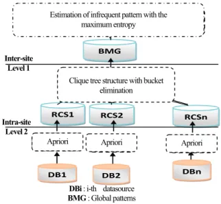
ROCESS

We are proposing our approach to determine the global itemset support from local itemsets in the process of multi data source mining. Interstate companies often consist of multi-level branches. In this paper we simplify each interstate company as a two-level organization with a centralized company headquarters and multiple branches, as depicted in Fig. 1. Each branch has its own database.

The proposed estimation process can be achieved in two phases, as shown in Fig. 1.

Fig. 1. Proposed approach

DBi : i-th datasource BMG : Global patterns RCSi: frequent itemset at site i Intra-site

Level 2 Inter-site

Level 1

Estimation of infrequent pattern with the maximum entropy

Clique tree structure with bucket elimination

(6)

Phase 1. Intra-site processing

1.1 Offline phase

Input: a binary transaction table (databases), minimum support minsup Output: All of the frequent itemsets for R

Algorithm: Apriori Phase 2. Inter-site processing Organization phase

Input: The frequent itemsets

Output: The joint probability distributions Structure: Clique tree method

Online phase

Input: Set of all frequent itemsets (in the form of joint probability for the distributions), conjunctive query Q.

Output : P x : the probability distribution of the query Q that contain the itemset x

Algorithm:

Choose the itemsets whose variables are all mentioned in x Call the scaling iterative algorithm for estimating P x Return : P x

3.1 Intra-Site Processing

In this step we applied an algorithm for discovering the frequent itemsets in all local sites (Level 2). We used the Apriori algorithm[23] to extract the set of frequent itemsets from each data source.

3.2 Inter-Site Processing

In this step we recursively applied the maximum entropy method, which estimates the infrequent itemsets at the central level (Level 1), in order to synthesize the global patterns.

The maximum entropy method can be used to define the markov random field (MRF), which is a stochastic process that is used to predict the future. As such, all useful information for predicting the future is contained in the state of this process. It is possible to represent the maximum entropy method as a product of the exponential functions that correspond to the cliques of the model graph H. The idea is to represent the joint probability distribution of frequent itemsets as tree cliques and to then apply the iterative scaling algorithm on this graph with the bucket elimination technique in each cluster of clique tree, which will reduce the time used in the maximum entropy method.

Thus, the application of the maximum entropy method to the query selectivity estimation is carried out in the following three steps:

Step 1. Construct the graph clique tree structure to gather the common distributions.

Step 2. Apply the iterative scaling algorithm as a convergence of maximum entropy solution in order to reduce the complexity estimation.

(7)

accelerate the estimation of common factors in the scale.

Our contribution for reducing the time complexity consists of combining the clique tree method with the bucket elimination technique by first decomposing the original problem into smaller ones and then processing each clique tree cluster by doing iterative scaling using the bucket elimination technique.

3.2.1 The clique tree method

A clique tree method is an undirected graph G = (V, E), which is a subset of the vertex set C ⊆ V, in such a way that for every two vertices in C, there is an edge (E) connecting together. This is equivalent to affirming that the sub-graph induced by C is complete.

The next paragraph covers how to build a graph clique tree with a set of frequent itemsets. Suppose that for a given query of Q, we have established a set of all itemsets that contain only variables occurring in the query Q. These itemsets define the undirected graphical model H on request variables with nodes corresponding to the query variables . A link connects two nodes if and only if the corresponding variables are mentioned in some itemset [9].

For example, consider a query on six binary attributes of A1-A6. Assume that there are frequent itemsets corresponding to each single attribute and that the following frequent itemsets are size 2: { A1=1, A2 = 1}, { A2=1, A3 = 1}, {A3=1, A4 = 1}, {A4=1, A6 = 1}, {A3 = 1, A5 = 1} and {A5=1, A6 = 1}. The graphical model H in Fig. 2 shows the interactions between the attributes in this example.

Fig. 2. The graphical model for the example

We first picked an ordering of the variables in the graph H and imposed triangulated graph in this ordering (i.e., we connected any two parents disconnected from any node [16]). The triangulated graph H’ is given in the Fig. 3.

Fig. 3. Triangulation of graph H’ for the example

A1 A2 A6 A5 A3 A4 A1 A2 A6 A5 A3 A4

(8)

For the triangulated graph, the joint probability distribution on the variables corresponding to vertices the triangulated graph can be decomposed into the product of probability distributions on the clique intersections. The maximal cliques of the graph are placed into a joint tree (a forest) that shows how cliques interact with each other. The clique tree in the example in Fig.2 is given in the following figure Fig. 4 :

Fig. 4. The clique forest corresponding to the problem in Fig. 2

Thus, the original problem is decomposed into smaller problems that correspond to the cliques of the triangulated graph H'. Every smaller problem can be solved separately by using the iterative scaling algorithm, while the distribution corresponding to the intersection can be found by adding up the corresponding distributions on the cliques. We used the iterative scaling algorithm for estimating the functions that correspond to cliques (joint probabilities) to estimate the support of infrequent itemsets from these functions.

3.2.2 Graduation as a convergence of iterative maximum entropy

The iterative scaling algorithm is well known in statistical literature as an technique which converges to the maximum entropy solution for problems of this general form.

The next paragraph describes how to calculate the probability estimate of .

Let the given query be Q. First, we consider only the itemsets whose variables are subsets of . Then denote these subsets by itemsets. It can be shown in [17] that the maximum entropy distribution is:

arg max ∈ (1) With ∑ log has the form of product:

∏

: ∈ (2) Where the constants μ0, ..., μj, ... are estimated from data. Once the constants are estimated as μj, Equation 2 can be used to estimate any query on the variables of and Q, in particular. The product form of the target distribution contains exactly one factor corresponding to each of the constraints. Factor μ0 is a normalized constant whose value is found from the condition of:

A3 A4 A5 A4 A5 A6 A2 A3 A1 A2 A2 A3 A4 A5

(9)

∑ ∈ , 1 (3) The coefficients μj are estimated by iteratively imposing each constraint in (3). The itemset ∈ defines a constraint as . Enforcing the j-th constraint can be carried by adding up all of the variables that are not participating in from and by requiring that the result of this sum equals the true account of for the itemset in the context. The constraint corresponding to the j-th itemset is:

∑ _{∈ ,} 1, … , 1 (4) where I (.) is the indicator function.

The iterative scaling algorithm is defined as described below [9].

The update rules for the parameter that corresponds to the j-th constraint at iteration t are: (5)

(6) ∑ (7) Equation 7 calculates the same constraints as in Equation 4 by using the current estimate , which is defined by the estimates of the through Equation 2. Addition is performed for all of the values of the query variables that satisfy the j-th itemset.

The iterative scaling algorithm proceeds in a round-robin fashion to the next constraint at each iteration. It can be shown that this iterative procedure converges to the unique maximum entropy solution provided the constraints on the distribution are consistent.

Detecting the convergence can be determined by various means and the algorithm stops when:

| Q Q | (8)

Where 10 indicate the free parameter.

Algorithm: iterative scaling

Input: Set of all T-frequent itemsets for R, Query Q. Output: Distribution

Algorithm:

1. Choose an initial approximation to (typically uniform)

2. While (Not all Constrains are Satisfied) For (j varying over all constraints) Update ;

Update ; End;

EndWhile; Output the constants

(10)

3.2.3 Bucket elimination

The bucket elimination technique can reduce the high computational complexity of iterative scaling. It accelerates the iterative scaling algorithm and estimates the common factors in the loop when updating factors using the distributive law in Equation 7. The advantage of this technique is illustrated on a simple example. Consider graph H in Fig. 2 and according to Equation 2, the maximum entropy distribution is:

. . ∏ ∏, ∃ , ∈

∗

Suppose that for the current iteration, we are updating the coefficient μ56 that corresponds to the itemset {A5=1, A6=1}. According to our update rule in Equation 7 we need to set the attributes A5 and A6 to 1 and sum out the rest of the attributes in . . .

After that we divide the functions μ involved in the computation into Buckets[9]. Each attribute ν defines a separate Bucket. The division factor for Buckets is illustrated as shown below.

Bucket ( )={ , };

Bucket ( )={ , , } ;

Bucket ( )={ , };

After the division of each bucket in the order process we used the following three basic steps that we applied consecutively: (a) multiplied all of the functions of each bucket, (b) required the variable outside of the Bucket, and (c) place the resulting function f into the topmost bucket mentioning any of the variable of f. Using bucket elimination allows us to reduce the number of terms evaluated by a factor of 2:

∑ .. . . , 1, 1= . ∑ . ∑

.( ∑ (∑ )))

Thus, the distributive law allows for an efficient execution time of the iterative scaling procedure.

With our approach we used the clique tree methods and applied the bucket elimination technique. As such, the maximum entropy distribution for this example is:

. . ∏ ∏, ∃ , ∈

(11)

We showed that the number of factors is reduced to 8, as compared with the maximum entropy, which has 13 factors.

We can assume that the complexity of our approach is Ο ∑ in space and is Ο 2 in time where:

: is the size of the clique tree : is the number of cliques

This is less than the complexity of the maximum entropy method, because < and < n , n are the size of the query and N is the number of itemsets.

We have illustrated our approach by using the example that is listed below. Step 1 : Intra-site processing

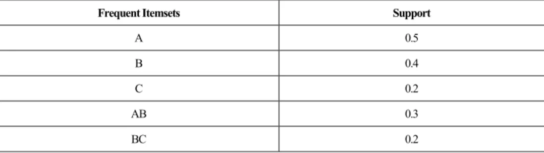
Let A, B, C, AB, and BC be the frequent itemsets obtained by the Apriori algorithm in the local site. Their support is shown in Table 1.

Table 1. Frequent itemsets discovered by the Apriori algorithm

Frequent Itemsets Support

A 0.5 B 0.4 C 0.2 AB 0.3 BC 0.2 Step 2: Inter-site processing

For estimating the support of infrequent itemsets ABC noted as sup(ABC), we build the clique tree as shown in Fig. 5.

Fig. 5. Clique tree corresponding to the problem in example

We applied the iterative scaling algorithm in this distribution as follows:

(12)

The result of the first iteration is as follows: -The factor

∗ =0.1532

0.2 ∗ _. . =0.19 0.3 ∗ . ∗_. _∗. _. = 0.416

Other factors estimation are: =0.466, =0.4, =0.4, =0.6351

The courant estimation: ABC = =0.019

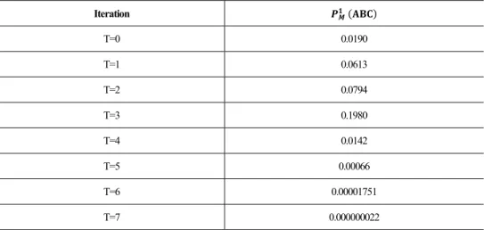
The table below summarizes the factor values for 8 iterations. Table 2. Factor values

Iteration T=0 0.0190 T=1 0.0613 T=2 0.0794 T=3 0.1980 T=4 0.0142 T=5 0.00066 T=6 0.00001751 T=7 0.000000022 Our algorithmwill finish when:

| Q Q | . The third iteration ABC 0.1980 is the maximum

estimation.

4. E

XPERIMENTS

In order to verify the effectiveness of our proposed method, we conducted some experiments. We chose a database “mushroom” that is available in: http://fimi.ua.ac.be/data/. The dense dataset contains 8,124 examples with 22 distinct items. For multi-database mining, the database is divided into four datasets, namely S1, S2, S3, and S4, with a transaction population of 2,500, 2,500, 1,624, and 1,500 respectively.

The frequent itemsets are discovered with the Apriori algorithm from: (a) A huge database that contains data from all datasets.

(b) The individual data sources with a minimum support (minsup) values of 0.5, 0.7, and 0.85 and with a minimum confidence (minconf) value of 0.30:

(13)

- Without making an estimate of the frequent local patterns

- With making an estimate of the frequent local patterns by employing factor correction[9].

- With making entropy method for estimate the frequent local patterns.

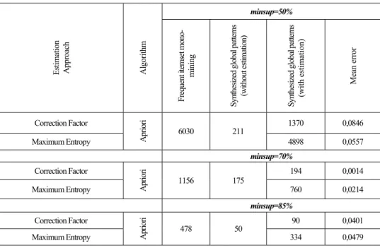
Table 3. Estimation approach (number of estimated itemsets and error means) for MinSup=0.5, 0.70, 0.85 Estimati on Appr oac h Algorit hm minsup=50% Frequen t item set m ono-m ini ng Synthesized glob al p atter ns (w ithout estim ation ) Synthesized glob al p atter ns (with esti mation) Me an e rro r Correction Factor Apr ior i 6030 211 1370 0,0846 Maximum Entropy 4898 0,0557 minsup=70% Correction Factor Apr ior i 1156 175 194 0,0014 Maximum Entropy 760 0,0214 minsup=85% Correction Factor Apr ior i 478 50 90 0,0401 Maximum Entropy 334 0,0479

The results obtained by the synthesized global patterns are compared with and without estimation support. They are also compared with the mono-database mining and with entropy estimation as shown in Table 3.

Table 3 contains the number of global frequent itemsets and error means for each method for different values of the minimum support (MinSup).

Error means= ∑ where - n is the number of estimated frequent itemsets. Error support |global support estimated itemset global support itemset | Total means error is the average of means error for the estimated itemsets support.

For example, let minsup=50%, the mono-database mining algorithm extracts 6030 frequent global itemsets. With the multi-databases mining algorithm, without make an estimate of local frequent itemsets, we only came up with 211 global frequent itemsets. These 6030-211=5819 patterns emerge as occurring frequently in some of the sites, but not in all. If we take these supports for infrequent itemsets, they will contribute to the global synthesizing process. Unfortunately, with the correction factor estimation [1] this number will be ameliorated because we found 1,370 global frequent itemsets. The number of global frequent itemsets increased by about 1,370-211=1,159 itemsets. However, we had a loss of 6,030-1,370=4,660 global frequent

(14)

itemsets, which represent about 77% of the frequent global itemsets that are ignored. With maximum entropy method [1] we can estimate 4898 frequent global itemsets, which represent 81% of the frequent global itemsets. We can show that the maximum entropy method gives nearly the same result as the mono-database mining.

The correction factor method gives the total means (0.0846+0.0014+0.0401)/3=0.042, which is higher than (0.0557+0.0214+0.038)/3=0.038 of the maximum entropy method. We can conclude that the support quality in the maximum entropy method is better than others methods.

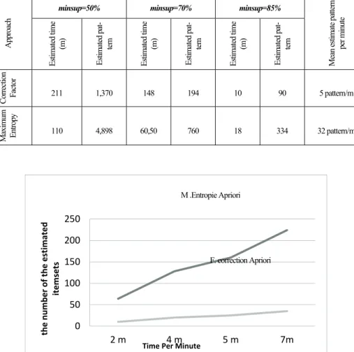
The times of different approaches are shown in Table 4 and Fig. 6 according to the different values of minsup and the number of estimated itemsets. Table 4 and Figure 6 describe the number of estimated patterns and the time of estimation by different approaches. It is clear that our approach is better than [1] because the mean pattern estimated for our approach is 32 pattern/minute while in [1] is 5 pattern/minute. Our approach is faster than the correction factor algorithm.

Table 4. The number of estimated patterns and the execution times

Appr

oach

minsup=50% minsup=70% minsup=85%

Me an es timat e p att er n per m inu te Es tima ted ti me (m) Est ima ted pa t-te rn Es tima ted ti me (m) Est ima ted pa t-te rn Es tima ted ti me (m) Est ima ted pa t-te rn Corr ection Fa cto r 211 1,370 148 194 10 90 5 pattern/m Max imu m E ntr opy 110 4,898 60,50 760 18 334 32 pattern/m

Fig. 6. The number of estimated patterns and the execution time 0 50 100 150 200 250 2 m 4 m 5 m 7m the number of the estimated itemsets

Time Per Minute

M .Entropie Apriori

(15)

From the previous results, we note the following items:

- The estimate of the frequent global patterns by the correction factor algorithm gives a good estimate of frequent global patterns, but it is slow and gives only 21% of the frequent global patterns for the mono-mining result.

- With the maximum entropy method, the synthesized results are nearly the same as the mono-mining results. It gives about 78% of the frequent itemsets for the mono-mining result.

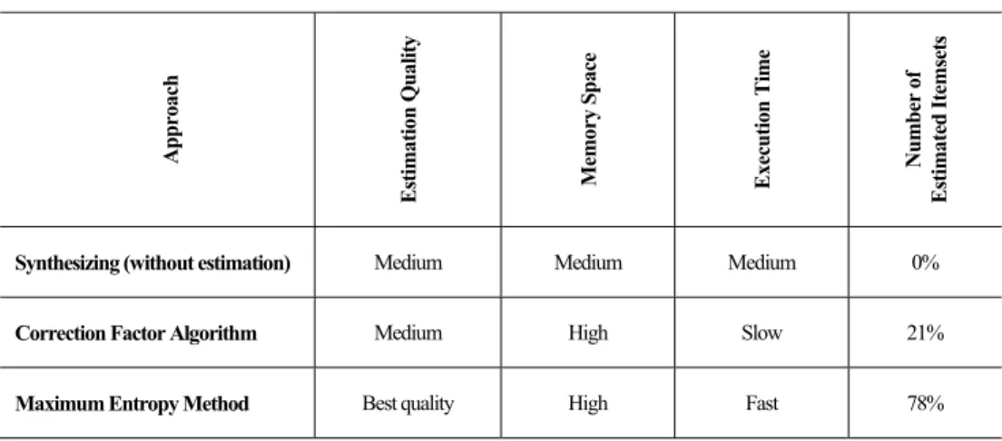
We can say that our estimation approach gives a good and fast estimation for a large number of estimated patterns from the frequent patterns that are generated by the Apriori algorithm. Table 5. Comparison of the different methods

Approach Estima tio n Qu alit y Mem ory Space Exec ution Ti me Number of Estima ted Itemset s

Synthesizing (without estimation) Medium Medium Medium 0%

Correction Factor Algorithm Medium High Slow 21%

Maximum Entropy Method Best quality High Fast 78%

5. C

ONCLUSION

This paper shows a method for synthesizing the global patterns by using a probabilistic model, with the goal of obtaining nearly the same global patterns as the mono-database mining. To achieve this end, we applied the maximum entropy method during the inter-site process and used both clique method and Bucket elimination technique in order to reduce the complexity of the maximum entropy method. The results show that the accuracy of results for the proposed synthesizing process is nearly the same as the mono-mining results.

Future work will be directed toward experiments using real-world datasets and for testing the system in real multi-databases. Also, we will test our approach in benchmark databases and especially in the sparse datasets and in others dense datasets.

R

EFERENCES

[1] Thirunavukkarasu Ramkumar, Rengaramanujam Srinivasan, « The Effect of Correction Factor in Synthesizing Global Rules in a Multi-databases Mining Scenario », Journal of computer science, no.6 (3)/2009, Suceava.

(16)

[2] Xindong Wu and Shichao Zhang, «Synthesizing High-Frequency Rules from Different Data Sources», IEEE TransKnowledge Data Eng 15(2):353–367 (2003).

[3] Thirunavukkarasu Ramkumar, Rengaramanujam Srinivasan, « Modified algorithms for synthesizing high-frequency rules from different data sources», Springer-Verlag London Limited 2008.

[4] Thirunavukkarasu Ramkumar, Rengaramanujam Srinivasan, «Multi-Level Synthesis of Frequent Rules from Different Data Sources», April, 2010.

[5] Shichao Zhang, Xiaofang You, Zhi Jin, Xindong Wu, «Mining globally interesting patterns from multiple databases using kernel estimation», (2009) .

[6] Shichao Zhang and Mohamed j. Zaki, « Mining Multiple Data Sources: Local Pattern Analysis», Data Mining Knowledge Discovery 12(2–3):121–125 ( 2006).

[7] Animesh Adhikari, P.R. Rao, « Synthesizing heavy association rules from different real data sources», Elsevier Science Direct 2008.

[8] Animesh Adhikari, Pralhad Ramachandrarao, Witold Pedrycz. Books, « Developing Multi-databases Mining Applications » chapter 3 “Mining Multiple Large Databases”, Springer-Verlag London Limited 2010.

[9] D. Pavlov, H. Mannila, and P. Smyth, « Beyond independence: Probabilistic models for query approximation on binary transaction data », Technical Report UCI-ICS-TR-01-09, Information and Computer Science, University of California, Irvine, 2001.

[10] V. Poosala and Y. Ioannidis, « Selectivity estimation without the attribute value independence assumption », In Proceedings of the 23rd International Conference on Very Large Data Bases (VLDB’97), pages 486–495. San Francisco, CA: Morgan Kaufmann Publishers, 1997.

[11] J. N. Darroch and D. Ratcliff, « Generalized iterative scaling for log-linear models », Annals of Mathematical Statistics, 43:1470–1480, 1972.

[12] Toon Calders and Bart Goethals, « Quick Inclusion-Exclusion », University of Antwerp, Belgium. Springer-Verlag Berlin Heidelberg 2006.

[13] Unil Yun, « Efficient mining of weighted interesting patterns with a strong weight and/or support affinity», Information Sciences 177 (2007) 3477–3499 Elsevier 2007.

[14] S. Jaroszewiez, D. Simovici and I.Rosenberg, « An inclusion-exclusion result for Boolean polynomial and its applications in data mining », In proceedings of the Discrete Mathematics in DM Workshop.SIAM DM Conference, Washington .D.C. 2002.

[15] Szymon Jaroszewiez, Dan A.Simovici, « Support Approximation Using Bonferroni Inequalities », University of Massachusetts at Boston, Departement of Computer Science USA.

[16] A.L. Berger, S.A. Della Pietra, and V.J. Della Pietra, « A maximum entropy approach to natural language processing », Computational Linguistics, 22(1):39–72, 1996.

[17] J. Pearl, « Probabilistic Reasoning in Intelligent Systems: Networks of Plausible Inference », Morgan Kaufmann Publishers Inc., 1988.

[18] F. Jelinek, « Statistical Methods for Speech Recognition », MTT Press.1998.

[19] D. Pavlov, H. Mannila, and P. Smyth, « Probabilistic models for query approximation with large Sparse Binary Data Set », Technical Report N°:00-07department of information and computer science, University of California, Irvine. February 2000.

[20] CHAIB Souleyman et MILOUDI Salim, «Fouille multi-bases de données : Analyse des motifs locaux», Master thesis, University of mohamed Boudiaf Oran Algeria 2011.

[21] H. Mannila and H. Toivonen, « Multiple uses of frequent sets and condensed representations », In Proc. KDD Int. Conf. Knowledge Discovery in Databases, 1996.

[22] H. Mannila, D. Pavlov, and P. Smyth, «Predictions with local patterns using cross-entropy », In Proceedings of Fifth ACM SIGKDD International Conference on Knowledge Discovery and Data Mining (SIGKDD’99), pages 357—361. New York, NY: ACM Press, 1999.

[23] C. K. Chow and C. N. Liu, «Approximating discrete probability distributions with dependence trees», IEEE transactions on Information Theory, IT-14(3):462-467, 1968.

[24] Rakesh Agrawal, Ramakrishnan Srikan « Fast Algorithms for Mining Association Rules » In VLDB’94, pp. 487-499.

[25] Jiawi Han, Jina Pei, Yiwen Yin, Runying Mao, «Mining Frequent Patterns without Candidate Generation: A Frequent-Pattern Tree Approach », Data Mining and Knowledge Discovery, 8:53-87, 2000.

(17)

[26] N. PASQUIER, Y. BASTIDE, R. TAOUIL, L. LAKHAL, «Efficient mining of association rules using closed itemSet », lattices. Information Systems, pages 25-46, 1999.

[27] Zhang S, Wu X, Zhang C., Multi-databases mining. IEEE Comput Intell Bull 2:5–13, 2003.

Mr. Khiat Salim

He holds a post graduation degree in computer science from University of science and technology–Mohamed Boudiaf Oran USTOMB Algeria in 2007. He teaches courses in undergraduate and graduate composition, at National School Polytechnic Oran Algeria.

He is memberships in Signal, System and Data Laboratory (LSSD).

His current research interests include the databases, multi-database mining for software engineering, Ontology, grid and cloud computing.

Pr. Hafida Belbachir

He Received PH.D degree in Computer Science from University of Oran, Algeria in 1990. Currently, she is a professor at the Science and Technology University USTO in Oran, where she heads the Database System Group in the LSSD Laboratory. Her research interests include Advanced DataBases, DataMining and Data Grid.

Dr. Sid Ahmed Rahal

He is Doctor in computer science since 1989 in Pau University France. He is memberships in professional activities are:

- Member of LSSD (Laboratory Signal, System and Data) - Interest in DataBases, Data Mining, Agent and expert systems.