HAL Id: tel-03021334
https://hal.archives-ouvertes.fr/tel-03021334
Submitted on 24 Nov 2020
HAL is a multi-disciplinary open access
archive for the deposit and dissemination of
sci-entific research documents, whether they are
pub-lished or not. The documents may come from
teaching and research institutions in France or
abroad, or from public or private research centers.
L’archive ouverte pluridisciplinaire HAL, est
destinée au dépôt et à la diffusion de documents
scientifiques de niveau recherche, publiés ou non,
émanant des établissements d’enseignement et de
recherche français ou étrangers, des laboratoires
publics ou privés.
Recovery
Isa Costantini
To cite this version:
Isa Costantini. Paradigm Free Regularization for fMRI Brain Activation Recovery. Signal and Image
processing. Inria Sophia Antipolis - Méditerranée, Université Côte d’Azur, 2020. English.
�tel-03021334�
ii
PHD THESIS
Paradigm Free Regularization for
fMRI Brain Activation Recovery
Isa COSTANTINI
Inria Sophia Antipolis – Méditerranée, Athena Project Team
Submitted in partial fulfillment
of the requirements for the degree
of Doctor of Science Specialized in
Automatic, Signal and Image Processing
of the Université Côte d’Azur
Advisor : Rachid Deriche
Co-advisor: Samuel Deslauriers-Gauthier
Defended on:
28 May 2020
In front of a Jury composed of:
Rachid Deriche, Inria Research Director,
Inria Sophia Antipolis - Thesis Advisor
Samuel Deslauriers-Gauthier, Inria
Sophia Antipolis - Thesis Co-advisor
Gloria Menegaz, Professor,
Università di Verona, Italia - Reviewer
Théodore Papadopoulo, Inria Research
Director, Inria Sophia Antipolis - Examiner
Maria Giulia Preti, Lecturer, MIPLab, EPFL &
Université de Genève, Switzerland - Examiner
Yuemin Zhu, CNRS Research Director
CREATIS Lab, INSA Lyon - Reviewer
iii
Summary
The advent of new brain imaging techniques such as resting-state functional MRI (fMRI), has led to the need for new approaches to recover brain functional activations without a prior knowledge on the experimental paradigm, as it was the case for task-fMRI. Conventional methods, i.e. the general linear model, requires the knowledge of the task paradigm to estimate the contribution of each voxel’s time course to the given task. To overcome this limitation, approaches to deconvolve the blood-oxygen-level-dependent (BOLD) response and recover the underlying neural activations without necessity of prior information has been proposed. Supposing the brain activates in constant blocks, first we propose a temporal regularized deconvolution technique which uses an exponential operator, whose shape and performance can be adjusted, into a least absolute shrinkage and selection operator (LASSO) model solved via the Least-Angle Regression (LARS) algorithm. We reduced the number of parameters to be set by the user, when compared with the state of the art. Second, we introduce a paradigm-free regularization algorithm that applies on the 4-D fMRI image, acting simultaneously in the 3-D space and the 1-D time dimensions. The approach is based on the idea that large image variations should be preserved as they occur during an activation, whereas small variations should be smoothed to remove noise. It allows to smooth the whole fMRI image with an anisotropic regularization, thus blindly recovering the location of the brain activations in space and their timing and duration. Both approaches were tested on phantom and real data and were demonstrated to improve the results obtained in the state of the art.
Keywords: BOLD, Deconvolution, Edge detection, Functional MRI, Hemodynamic Response Function, Image Regularization, Paradigm Free, Partial Diferential Equations, Resting-state
v
Resumé
L’avènement de nouvelles techniques d’imagerie du cerveau comme l’IRM fonctionnelle (IRMf) au repos a conduit à la nécessité de nouvelles méthodes pour récupérer les activations fonctionnelles du cerveau sans connaissance du paradigme expérimental, comme dans l’IRMf basée sur tâche. Les méthodes conventionnelles, par example le modèle linéaire général, nécessitent la connaissance de la tâche pour pouvoir estimer la contribution du signal de chaque voxel à la tâche donnée. Pour surmonter ces limitations, des méthodes de déconvolution de la réponse dépendant du niveau d’oxygène dans le sang et de récupération des activations neurales sans avoir besoin d’informations préalables ont été proposées. Dans cette thèse, nous proposons d’abord une technique de déconvolution avec une regularisation temporelle qui utilise un opérateur exponentiel, dont la forme et la performance peuvent être ajustées. Avec cette méthode, nous avons réduit le nombre de paramètres à régler par l’utilisateur, par rapport à l’état de l’art. Ensuite, nous avons introduit un algorithme de régularisation qui s’applique à l’image IRMf 4-D, agissant simultanément dans les dimensions spatiale et temporelle. La méthode est basée sur l’idée que les grandes variations de l’image doivent être préservées car elles se produisent lors d’une activation et les petites variations doivent être lissées pour éliminer le bruit. Elle permet de lisser l’image IRMf avec une régularisation anisotrope, récupérant ainsi aveuglément la localisation des activations cérébrales et leur durée. Les deux méthodes ont été testées sur des données synthetiques et réelles et ont démontré une amélioration des résultats de l’état de l’art.
Mot-clés: IRMf - Activation Cérébrale - Reconstruction Régularisée – Regularisation Anisotropique
vii
Acknowledgements
This work has received funding from the European Research Council (ERC) under the European Union’s Horizon 2020 research and innovation program (ERC Advanced Grant agreement No 694665: CoBCoM - Computational Brain Connectivity Mapping).
Data were provided [in part] by the Human Connectome Project, WU-Minn Consortium (Principal Investigators: David Van Essen and Kamil Ugurbil; 1U54MH091657) funded by the 16 NIH Institutes and Centers that support the NIH Blueprint for Neuroscience Research; and by the McDonnell Center for Systems Neuroscience at Washington University.
ix
Contents
Summary iii
Resumé v
Acknowledgements vii
List of Figures xiii
List of Tables xxi
List of Abbreviations xxiii
Part I – Introduction
1
Introduction 3
Context . . . 3
Problem. . . 3
Contributions and List of Publications . . . 4
Software Contributions . . . 6
Organization of the Thesis . . . 6
Part II – Background
9
1 From Neurons to BOLD-contrast imaging 11 1.1 Brain Biology, Anatomy and Physiology . . . 111.1.1 Brain Cellular Structure . . . 11
1.1.2 Human Brain Anatomy . . . 12
1.1.3 Human Brain Function. . . 14
1.2 Introduction to NeuroImaging . . . 17
1.3 Fundamentals of MRI. . . 18
1.3.1 The Echo Planar Imaging (EPI) Sequence . . . 20
1.4 Basic Principles of Functional MRI . . . 21
1.4.1 The Blood Oxygenation Level Dependent (BOLD) Contrast Imaging . 22 1.4.2 Sources of Noise in fMRI Images . . . 23
1.4.3 Standard Minimal Preprocessing of fMRI Data . . . 23
1.5 fMRI Techniques: Task and Resting-State fMRI . . . 25
Part III – State of the Art
27
2 fMRI Data Analysis 29
2.1 The General Linear Model . . . 29
2.2 Deconvolution of the fMRI BOLD Signal. . . 31
2.3 Voxel/Seed-based Methods . . . 35
2.4 Data-driven Approaches . . . 35
The Principal Component Analysis . . . 36
The Independent Component Analysis . . . 36
Clustering approaches . . . 38
2.5 Conclusion . . . 40
2.5.1 Limitations of the Current State of the Art. . . 40
Part IV – Contributions
41
3 fMRI Deconvolution via Temporal Regularization using a LASSO model and the LARS algorithm 45 3.1 Introduction to Inverse Problems and Regularization Approaches . . . 453.1.1 The Forward Model . . . 46
3.1.2 The Regularization Approach . . . 46
3.2 fMRI Image Structure. . . 48
3.2.1 The Hemodynamic Response Function . . . 48
3.3 The Forward Model of fMRI Data . . . 52
3.4 L1-norm Temporal Regularized Deconvolution of the fMRI BOLD Signal. . . 52
3.4.1 Definition of LASSO Optimization Problem. . . 52
3.4.2 The α-Filter Design . . . 53
3.4.3 Solution of the LASSO problem using the LARS Algorithm and L-Curve 56 3.4.4 Leave-one-out Cross-Validation . . . 57
3.5 Simulation of fMRI Time-Courses . . . 59
3.6 L-curve vs Cross-Validation . . . 61
3.6.1 Methods . . . 61
3.6.2 Results . . . 61
3.7 Validation on Phantom fMRI Images . . . 68
3.7.1 Methods . . . 68
3.7.2 Results . . . 69
3.8 Application on Real task-fMRI Data . . . 72
3.8.1 Methods . . . 72
3.8.2 Results . . . 73
3.9 Discussion and Contributions of this Chapter . . . 73
3.10 Publications Arising from this Contribution . . . 75
4 A Paradigm Free Regularization Approach to Recover Brain Activation from fMRI Data 79 4.1 Spatio-Temporal Deconvolution of the fMRI BOLD Response. . . 79
4.2 Introduction to the Diffusion Process . . . 80
4.3 Image Regularization with Partial Differential Equations . . . 80
xi
4.5 Simulation of a Whole Brain fMRI Image . . . 84
4.6 Validation on phantom fMRI data. . . 85
4.6.1 Methods . . . 85
4.6.2 Results . . . 85
4.7 Validation on real fMRI data . . . 92
4.7.1 Methods . . . 92
Validation on task-fMRI Data . . . 92
Application on Resting-State fMRI Data . . . 93
4.7.2 Results . . . 94
4.8 Discussion and Contributions of this Chapter . . . 99
4.9 Publications Arising from this Contribution . . . 99
4.10 Application of the PF-fMRI Approach . . . 100
4.11 Software Contribution . . . 100
Part V – Conclusion
101
5 Concluding Remarks and Open Problems 103
Appendices
106
A α-Filter Design 109
B Application of the PF-fMRI Approach 119
C Contributions outside the scope of this thesis 121
xiii
List of Figures
1.1 Neurons structure and process of synaptic transmission. The figure shows how the neurons are composed and connected to each other. The cell body contains the nucleus and cytoplasm. The axon extends from the cell body and gives rise to small branches before ending at nerve terminals. Dendrites extend from the neuron cell body and carry the information between neurons. Synapses are the points where the "communications" between neurons take place. Figure taken from [1] . . . 13 1.2 Conventional terminology which indicates the different orientations
representing the different brain views: in surface (A), section (B) and connectional anatomy (C). Surface neuroanatomy is the one describing the appearance of grooves (sulci) and folds (convolutions or gyri) of the brain. Sectional neuroanatomy illustrates the cortical and subcortical structures and their relationship, commonly described along the axial, coronal and sagittal plane. The connectional neuroanatomy desribes the connecting fiber tracts’ origin, paths and terminations. Figure taken from Catani and Thiebaut de Schotten [2]. . . 15 1.3 Brain lobes of a dorsolateral (A) and medial (B) surface of the left cerebral
hemisphere. Solid lines show the main sulci dividing the lobes, while dashed lines represent arbitrary lines of separations which are following a sulcus. The gyri of each lobe are also illustrated. Figure taken from Catani and Thiebaut de Schotten [2]. . . 16 1.4 Longitudinal and transverse relaxation. T1 corresponds to the time in
which the longitudinal component regain a value which is the 37% lower of its equilibrium value; T2 corresponds to the time in which the transverse component is reduced to the 37% of it. Figure taken from Pizzolato [3]. . . 20 1.5 Examples of MRI brain scans in the axial plane: T1-weighted (left) and
T2-weighted images (right). . . 21 1.6 Echo Planar Imaging (EPI) Sequence – (A) EPI sequence with phase-encoding
along y direction using blipped gradient pulses. (B) Trajectory of the EPI sequence in the k-space. The different colors of the trajectories refer to the gradients Gxand Gy. . . 22
1.7 Schematic illustration of the generation of the blood-oxygen-level-dependent (BOLD) signal. Figure adapted from Iannetti and Wise [4]. . . 23 1.8 Hemodynamic response function (HRF) to a stimulus with a short duration,
illustrated with the red bar. The peak related to the blood-oxygen-level-dependent (BOLD) effect starts to increase after approximately 3 s from the stimulus starting point. Figure taken from Amaro and Burker [5]. . . 24
1.9 Example of functional MRI (fMRI) brain scans. Each image represent a scan of fMRI data, consecutively acquired in time (t). The images are represented, from left to right, in their sagittal, coronal and axial planes. . . 24
2.1 The approach of the general linear model (GLM). Each time series of fMRI data (Y) is a linear combination of regressors, composed both of task-related regressors (green) and nuisance regressors (light green) weighted by β, and the error e. The goal of the GLM is to minimize the error thus estimating the parameters weights β. . . . 30 2.2 fMRI signal model. From left, us(i, t) is the spike train (innovation signal)
which induces the activation for each voxel i. us(i, t)is the derivative of u(i, t)
which represents the activation and it is assumed to be a block-type signal. h(t)is the hemodynamic response function, that convolved with the activity-inducing signal u(i, t)gives the activity-related signal x(i, t). y(i, t)represents the measuref fMRI signals for each voxel i, which is obtained by adding noise to the activity-related signal. (Figure adapted from Karahano ˘glu et al. [6]). . 33 2.3 13 innovative-driven co-activation patterns (iCAPs) ordered with respect to
their occurrence during a resting-state fMRI acquisition. The iCAP 1 contains auditory regions; the iCAP 2 includes regions of the fronto-parietal attention network; the iCAP 3 as well as the iCAP 4 cover the primary and secondary visual areas; the iCAPs 5 reveals the precuneus, the posterior cingulate cortex and the thalamus; the iCAP 6 represents the visuospatial/dorsal attention network; the iCAP 7 covers the motor network and the medial fromtal gyrus; the iCAP 8 corresponds to posterior part of the DMN; the iCAP 9 includes the anterior executive network; the iCAP 10 shows again a posterior part of the DMN; the iCAP 11 reveals the anterior salience network; the iCAP 12 is composed by the combination of different regions which are located in the limbic and the subcortical area, superior and middle temporal and occipital gyrus; the iCAP 13 contains the frontal gyrus, the anterior cingulate cortex and caudate. Figure adapted from Karahano ˘glu and Van De Ville [7]. . . 34 2.4 Seed-based method – To examine the time series and extract meaningful
information from fMRI data, i.e. the functional connectivity level between a seed voxel and another brain voxel i, the correlation between the two time series showed on the bottom right of the figure are computed. Highly correlated time courses reflect a high level of functional connectivity. To map all the functional connections of the seed and obtain the map showed at the bottom left of the figure, a voxel-wise correlation between the seed voxel’s time series and all the other brain voxels is calculated. The outcome is a map that shows which areas show a high level of functional connectivity with the selected seed [8]. Figure taken from Hu and Zeng [9]. . . 35 2.5 Matrix representation of the spatial indepenedent component analysis
(spatial-ICA). In spatial-ICA, the algorithm try to estimate spatially independent components with related time series. . . 37
xv
2.6 Different probabilistic independent component analysis (probabilisti-ICA)-estimated resting state outputs. Estimated from a group of 10 subjects, the eight spatial maps, coregistered and superimposed to the Montreal Neurological Institute (MNI) template, shows the sagittal, coronal and axial views of different components associated with low-frequency resting-state patterns. R: right; L: left. Figure adapted from Beckmann and colleagues [10]. 39
3.1 Representation of the 4-D functional MRI (fMRI) data. A fMRI image is composed by a set of 3-D volumes recorded over time, thus leading to a 4-D structure. TR = repetition time. Figure adapted from [11]. . . 49 3.2 From top left, following the black lines connecting the different plots,
s(t) is the spike train (innovation signal) which induces the activations.
Iα is the exponential accumulation function that leads from s(t) to the activity-inducing signal u(t), which is piece-wise constant. Hrepresents the hemodynamic response function, x(t) is the activity-related signal, ea is the
additive noise and y(t) is the simulated acquired fMRI time course. . . 54 3.3 Impulse response of the accumulation functionIα. The plot shows how the
accumulator changes increasing α, e.g. from 0.2 (green) to 1 (blue). . . . 55 3.4 L-curve. The graph represents for one time series of one voxel the plot of the
two quantities, one related to the norm of the solution (abscissa) and the other related to the residuals (ordinate), i.e. (||ˆs||1,||y− Aˆs||22), paramtrized by the
regularization parameter λ. Each black dot in the curve is related to each λ outputted by the Least Angle Regression (LARS) algorithm [12]. The red dot represents the optimal solution as the nearest to (0, 0)∈ R2.. . . 56 3.5 fMRI signal simulation. u(t)is the activity-inducing signal, a block of constant
activation represented with a piece-wise constant signal. eb is the block type
noise and emthe model noise which were consecutively added to the
activity-inducing signal u(t) thus leading to un(t) before the convolution with the
hemodynamic response functionH. x(t)is the activity-related signal, eais the
additive gaussian noise and y(t)is the simulated acquired fMRI time course. 60 3.6 Each plot shows the root mean square errors (RMSE) and the roots of standard
deviations computed between the ground truth activation and the estimated one using the Least Angle Regression (LARS) combined with the L-curve (in red) and with the leave-one-out cross-validation (LOO-CV, in light blue). Each plot refer to a different experiment, as reported in Table 3.3. For each experiment, the RMSE were averaged across 100 repetitions of the simulated time series. The errors (in y-axes) are plotted with respect to the α value (in x-axes) used for the α-filter. In the 5 experiments, we added block-type noise (eb)for false activations, and both em and ea to the data, increasing it from
experiment 1 to 5. The plots show that the LOO-CV-bases approach is more sensitive to noise while increasing it and results are more disperse if compared with the curve-based ones. In all experiments the results obtained with L-curve show errors that are significantly lower than those given by the LOO-CV. With respect to the parameter α, results obtained via the LOO-CV are improved by increasing it, instead the ones obtained with L-curve are more stable with respect to it. . . 64
3.7 Each plot in the figure show the root mean square errors (RMSE) and the roots of standard deviations computed between the ground truth activation and the estimated one using the Least Angle Regression combined with the L-curve (in red) and with the leave-one-out cross-validation (LOO-CV, in light blue). Each plot refer to a different experiment, as reported in Table 3.3. For each experiment, the RMSE were averaged across 100 repetitions of the simulated time series. The RMSE (in y-axes) are plotted with respect to the α value (in x-axes) used for the α-filter. In experiments from 6 to 10, we increasingly added eato the synthetic times series. The plots show that the LOO-CV-based
approach is less sensitive to noise if compared to experiments 1 to 5 in Figure 3.6, but still more sensitive to noise while if compared with the L-curve-based ones. In all experiments the results obtained with L-curve show errors that are significantly lower than the ones obtained with the LOO-CV for α values lower than 0.5. For α>0.75 results are similar. . . 65 3.8 The graphs in the plots show examples of the recovered activation using
the mixed Least Angle Regression (LARS)-L-curve approach (in red) and the mixed LARS and leave-one-out cross-validation (LOO-CV) (in light blue) superimposed on the ground truth activation in black and the noisy synthetic fMRI time series (in green). Each row shows a different experiment, meaning different noises applied to the ground truth activation and each columns refer to a specific α used in the α-filter. In experiments 1, 3 and 5 the added noise was coming from different sources: block-type noise (eb) to simulate
false-activations, model noise emand additive noise ea. The standard deviations of
emand eaincreases from experiment 1 to 5. The plots show that the recovered
activations using the L-curve-based approach are much closer to the ground truth compared with LOO-CV. The L-curve-based approach shows results that are closer to the ground truth in terms of amplitude for bigger alphas. For
α=0.75, 3, results are similar, while in contrast with those given by α=0.3. 66
3.9 The graphs in the plots report examples of the recovered activation using the mixed Least Angle Regression (LARS)-L-curve approach (in red) and the mixed LARS and leave-one-out cross-validation (LOO-CV) (in light blue) superimposed on the ground truth activation in black and the noisy synthetic fMRI time series (in green). Each row shows a different experiment (see Table 3.3), meaning that different amount of noises were applied to the ground truth activation Each columns refer to a specific α used in the α-filter. In experiments 6 and 10 time series are corrupted with eawith increasing standard deviation.
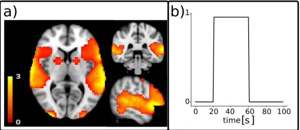
The different amount of noise are described in Table 3.3. The recovered activations using the L-curve-based approach are closer to the ground truth compared with LOO-CV. The L-curve-based approach shows results that are closer to the ground truth in terms of amplitude for greater alphas α=0.75, 3, in contrast with α=0.3. . . 67 3.10 3-D activation map obtained from an auditory task superimposed on the
standard Montreal Neurological Institute (MNI) brain. The three images, from left to right, represent the axial, the sagittal and the coronal view. Voxels’ intensity is ranged between 0 and 3. . . 68
xvii
3.11 Piece-wise constant activity-inducing signals simulated for validation. The activation on the left, A, is composed by four blocks of activations with different durations, as proposed by Farouj et al. [13]. The activation on the right, B, is made of a single long block of simulated activity. . . 68 3.12 Reconstructed activity-inducing signal ˆu(t)obtained with our approach (red)
superimposed on the ground truth (u(t), black) and simulated fMRI signal (y(t), green). The plots in the blue square are taken from exemplificative voxels and are related to activation A with pSNR = 5.17 dB; the ones in the yellow square are related to activation B with SNR = 5.12 dB. Vertically, for both A and B, the plots show that our approach is able to discern between an activation and a non-activation. . . 70 3.13 Reconstructed activity-inducing signal ˆu(t) obtained with our approach
(red) and the total activation (TA, blue) superimposed on the ground truth activation (black) and simulated fMRI signal (green). The plot on the top is related to activation A with pSNR = 5.17 dB. The plot on the bottom is related to activation B with pSNR = 5.12 dB. . . 71 3.14 The plot shows the ˆu(t) obtained with the Human Connectome Project
(HCP) data. Results obtained using our approach (red) and the TA (blue) superimposed on the real fMRI signals (green) were all averaged within the region of interest located in the Broadmann Area 4p. In the x-axes the time is expressed in TRs and the gray areas represent the duration of the tongue movements. . . 74
4.1 Ellipsoidal representation of the 3-D diffusion tensor. . . 82 4.2 Ground truth for the functional MRI (fMRI) simulated data: (a) activation
map. (b) Simulated activation u(t), with a repetition time (TR) of 1 s. . . 85 4.3 (a) From left to right: spatial maps of the simulated functional MRI (fMRI)
image y, ground truth activation u, recovered activation using the Total Activation (TA) approach ( ˆuTA) and our approach ( ˆuPF− f MRI). Each row
corresponds to a a different peak-SNR (pSNR): 6.54 dB, 5.99 dB, 5.9 dB, 3.93 dB from the top to the bottom. (b) Reconstructed time series ˆu(t)obtained with our approach ˆuPF− f MRI(t) (red) and the TA approach ˆuTA(t) (blue)
superimposed on the ground truth activation u(t) (black) and fMRI signal y(t)(green). A zoom of the plot is shown in Figure 4.4. . . 87 4.4 The plot is a zoom of Figure 4.3 representative of a trend that we found in
all the four experiment showed in Figure 4.3. From top left: spatial maps of a slice of the simulated functional MRI (fMRI) image y, ground truth activation u, recovered activation maps obtained using the Total Activation (TA) approach ( ˆuTA) and the PF-fMRI ( ˆuPF− f MRI). The map obtained using
TA ( ˆuTA) had lower amplitude compared with the ground truth, nonetheless
the scale between the values were kept. The map obtained using PF-fMRI ( ˆuPF− f MRI) showed amplitude comparable to the ground truth, the scale
between the values were kept. The time series on the bottom shows that the recovered signal ˆuPF− f MRI(t)(red) was closer to the ground truth u(t)(black)
4.5 The graph shows, for different peak-SNRs, the roots of the mean square errors (MSE) and standard deviation (STD) between u(t)and ˆu(t)averaged among the voxels belonging to the gray matter. . . 89 4.6 The graph shows, for different peak-SNRs (pSNRs), the Pearson correlation
coefficient computed between u(t)and ˆu(t)and averaged among the voxels belonging to the gray matter and their standard deviation. (µr: mean
correlation coefficient; σr: standard deviation of the correlation coefficients.) . 89
4.7 (a) From left to right: spatial maps of the simulated functional MRI (fMRI) image y, ground truth activation u, recovered activation using our approach ( ˆuPF− f MRI). Each row corresponds to a different peak-SNR (pSNR):'0 dB,
-6.51 dB, from the top to the bottom. (b) Reconstructed time series obtained with our approach ˆuPF− f MRI(t) (red) superimposed on the ground truth
activation u(t)(black) and the original fMRI signal y(t)(green). . . 90 4.8 The graph shows, for different peak-SNRs (pSNR), the roots of the mean
square errors (MSEs) and standard deviation (STD) between the ground truth signal u(t)and the recovered signals ˆuPF− f MRI(t)averaged across the voxels
belonging to the gray matter. . . 91 4.9 The graph shows, for different peak-SNRs (pSNRs), the Pearson correlation
coefficient computed between the ground truth signal u(t)and the recovered activation ˆuPF− f MRI(t)averaged over the voxels belonging to the gray matter
and their standard deviation. (µr: mean correlation coefficient; σr: standard
deviation) . . . 91 4.10 Qualitative comparison between the General Linear Model (GLM) and our
approach (PF-fMRI). On the left column, in a blue-lightblue color-map, superimposed to the standard Montreal Neurological Institute (MNI) brain, the β-regressors map obtained using the GLM implemented in the FMRIB Software Library (FSL) tool. On the right column, in a red-yellow color-map, the whole-brain voxel-wise correlation maps obtained using the PF-fMRI superimposed to the standard MNI brain. The Pearson correlation was computed voxel-wise among the whole brain, between the reconstructed activity inducing signals ˆu(t)and the five motor tasks simulated as piece-wise constant signals with ones in the time points where the subject is executing a task and zeros elsewhere. The values r of the correlations are indicated by the color-bars. Each row corresponds to a specific motor task, from top to bottom: the tongue, the right and left hand, and the right and left foot. A: anterior; P: posterior; S:superior; I: inferior; R: right; L: left. . . 95 4.11 Barplots of the mean (µr)±standard deviations (σr) of the Pearson correlation
coefficients (r) computed on the sample data of 51 subjects in 5 ROIs related to the tasks of the left and right hand, the tongue end the left and right foot. For each task, the bars in red represents the results using the PF-fMRI for an increasing number of iterations (from 1 to 40). The blue bar represents the results obtained with the Total Activation (TA) approach. The black lines are the standard deviations (σr). (lHAND: left hand; rHAND: right hand; lFOOT:
xix
4.12 a) Reconstructed signals ˆu(t)obtained with our approach (PF-fMRI, red) and the total activation tool (TA, blue) superimposed on the real acquired fMRI signals (green). The ground truth in this case corresponds to the task (black), simulated as piece-wise constant signals with ones where the subject was asked to perform the task and zeros elsewhere. The plot on the top is related to the region of interest (ROI) located on the Brodmann Area 4p (rBA4p), the plot on the bottom is associated to the ROI positioned on the primary auditory cortex (rTE1.2). All the signals were averaged across the voxels belonging to the gray-matter (GM)-masked ROIs. The grey areas represent the occurrence and the duration of the tongue movements. b) Simulated tongue activation. c) Mean Pearson correlation coefficients (µ) and their associated standard deviations (σ) computed between the tongue activation and the recovered signals ˆu(t) averaged across the voxels belonging to the GM-masked ROIs (rBA4p on the left, rTE1.2 on the right). The blue curves are related to the TA
approach, while the red one to the PF-fMRI approach. TR: repetition time. . . 97
4.13 Each row in the figure shows for different iterations of the PF-fMRI approach, specifically the 5th, the 15th and the 45th iterations, the reconstructed signals (in red) obtained with our approach superimposed on the real resting state fMRI signals (in green). The activity-inducing signals ˆu(t)recovered via the PF-fMRI were averaged in a ROI located on the default mode network and masked using the gray matter mask. . . 98
A.1 Function h(n)defined in Eq. (A.1), for S= −1 and α=1. . . 110
A.2 Function g(n)defined in Eq. (A.15), for S= −1 and α=1. . . 113
A.3 FunctionIα(n)defined in Eq. (A.13), for S= −1 and α=1. . . 113
A.4 Function g(n) defined in Eq. (A.15), for S = −1 and α = 1. The plot shows that −1∑ n=−∞g(n) is equal to +∞ ∑ n=0 g(n). This means that, if we compute +∞∑ n=−∞g(n) = −1 ∑ n=−∞g(n) + +∞ ∑ n=0 g(n)this is equivalent to +∞∑ n=−∞g(n) = 2+∞∑ n=0 g(n). . . 115
A.5 The plot shows for different values of α the function Iα(n) defined in Eq. (A.13), normalized by the factor S defined in Eq. (A.35). The graphs show that for greater values of α, the filter is sharper, whereas if α is smaller, the filter has a smoother shape. . . 118
B.1 Illustration of the Desikan–Killiany atlas (A), functional MRI priors (B), and thresholded functional MRI priors with activation above 0.83 (C). The remaining regions are those used to select connections introduced into the proposed Bayesian network which are illustrated in D. . . 120
xxi
List of Tables
1.1 T1and T2relaxation times for brain tissues, gray matter and white matter, at
3 Tesla [14].. . . 19
3.1 Variables involved in the hemodynamic model [15,16]. . . 50 3.2 Constants involved in the hemodynamic model [15,16].. . . 50 3.3 Experiments set for testing the L-curve and the LOO-CV to compare the two
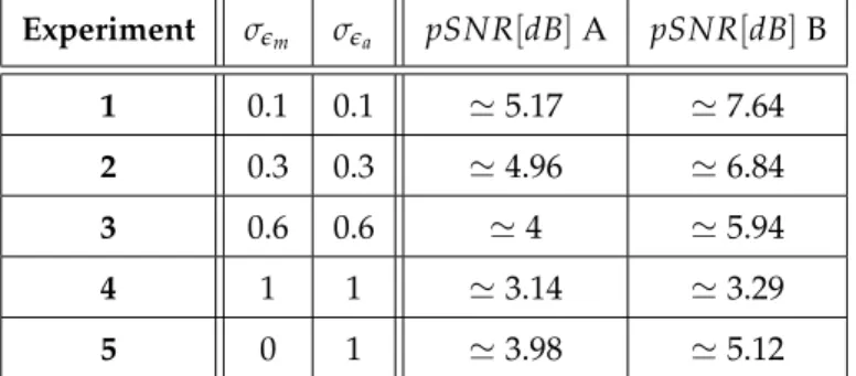
approaches for the selection of optimal lambda. The first column indicates the experiment number, the second column the standard deviation (σem) of the gaussian random noise added as model noise, the third column represents the peak signal to noise ration (pSNRm) computed as in (3.28) in dB. The fourth
column reports the σea for the additive gaussian noise and the fifth column the pSNRaestimated as in (3.29) expressed in dB. . . 62
3.4 Experiments set for testing our temporal regularized deconvolution on phantom fMRI image. The first column indicates the experiment number. The second and third columns report the standard deviation of the model noise (σem) and the additive gaussian noise (σea), respectively. The fourth and fifth columns show the pSNR computed as in (3.30), expressed in dB, for activations A and B. . . 69 3.5 Summary of rooted MSEs and STDs obtained for phantom fMRI data. . . 70 3.6 Tongue task paradigm of HCP data. Note that the time for activation is
expressed in seconds and the repetition time for the HCP data is 0.72s. . . 73
4.1 Motor task paradigm of HCP data. The time is expressed in seconds and the repetition time for the HCP data is 0.72s.. . . 92 4.2 MNI coordinates centers of the brain areas found to respond to the
somatosensory stimulation. The coordinates, adapted by Roux et al. [17] are expressed in MNI standard space. . . 93
xxiii
List of Abbreviations
1-D 1 Dimensional 3-D 3 Dimensional 4-D 4 Dimensional BA Brodmann AreaBOLD Blood Oxygen Level Dependent
CNS Central Nervous System
CSF CerebroSpinal Fluid
CT ComputedTomography
dMRI diffusion Magnetic Resonance Imaging
DMN Default Mode Network
EEG Electro Encephalo-Ggraphy
EPI Echo Planar Imaging
FA Flip Angle
FISTA Fast Iterative Shrinkage-Thresholding Algorithm
fMRI functional Magnetic Resonance Imaging
FMRIB Functional Magnetic Resonance Imaging of the Brain
FOV Field Of View
FSL FMRIB Software Library
GE Gradient Echo
GFB Generalized Forward-Backward
GLM General Linear Model
GM Gray Matter
gTV generalized Total Variation
HCP Human Connectome Project
HRF Hemodynamic Responce Function
ICA Independent Component Analysis
iCAP innovative-driven Co-Activation Pattern
ISTA Iterative Shrinkage Thresholding Algorithm
LASSO Least Absolute Shrinkage and Selection Operator
LARS Least Angle Regression
LOO-CV Leave One Out Cross Validation
MEG Magneto Encephalo-Ggraphy
MNI Montreal Neurological Institute
MSE Mean Squared Error
MR Magnetic Resonance
MRI Magnetic Resonance Imaging
NIRS Near Infrared Spectroscopy
PCA Principal Component Analysis
PDE Partial Differential Equation
PET Positron Emission Tomography
PF-fMRI Paradigm Free functional Magnetic Resonance Imaging
pSNR peak Signal-to-Noise Ratio
RF Radio Frequency
rs-fMRI resting state functional Magnetic Resonance Imaging
RF Radio Frequency
ROI Region Of Interest
RSN Resting State Network
SE Spin Echo
SNR Signal-to-Noise Ratio
SPM Statistical Parametric Maps
SPECT Single Photon Computed Tomography
T Tesla TA Total Activation TE Echo Time TR Repetition Time TV Total Variation WM White Matter
1
Part I
3
Introduction
Context
With the innovation introduced with the advent of neuroimaging techniques, new insights into the understanding of the functioning of the human brain have been possible. The human brain is the most interesting, fascinating as well as mysterious organ of the human body. It is where the mind and the intelligence, the soul and the personality, the thoughts and the behaviour as well as the functions that regulates and allows the movement of the entire human body are created and directed. Nonetheless, the brain does this starting from its basic component, the neuron, in a scale of microns and moreover it does it via simple electrical signals. Furthermore, the understanding of the brain becomes crucial to treat the neurodegenerative diseases due to the increased life expectancy of the population in the world. The ultimate goal of the neuroimaging community is to decode these signals and understand how the brain works and is organized while it is working, in a living human being, in other words in vivo.
Nowadays, there are several imaging modalities available and they can be classified into two main categories: the structural and functional neuroimaging modalities. (i) Magnetic Resonance Imaging (MRI) is a unique tool that provides anatomical images of the brain tissues. (ii) Functional MRI (fMRI) allows to obtain information about the brain function and how the different regions of the brain interact and integrate by exploiting a natural endogenous contrast of the properties of the blood oxygenation. (iii) Diffusion MRI (dMRI) instead allows the study of the white matter (WM) fiber bundles, hence the tracts connecting one brain region to another. (iv) Near-infrared spectroscopy (NIRS) gives information about regional oxygenation and blood flux via near-infrared region of the electromagnetic spectrum. (v) Magneto-and Electro-encephalography (MEG/EEG) perform measurements of the brain electro-magnetic activity. (vi) Computed Tomography (CT) allows 3-D scannings of the brain using x-rays. (vii) Position Emission Tomography (PET) gives information about the metabolic activity of the brain.
Neuroimaging modalities give indirect and degraded measures of the brain activity or structure, meaning that the acquired signals are corrupted by noise, and have to be interpreted using sophisticated analysis methods which allow to extract meaningful information.
Problem
The problem we are addressing in this thesis is the recovery of brain functional activations from fMRI data. Traditional techniques for measuring the brain function are based on experimental paradigms, where the subject is asked to perform a task in order to measure the difference between the rest condition, representing a baseline, and the task condition.
fMRI data analysis methods, i.e. the general linear model (GLM), require the knowledge of the task paradigm to be able to estimate the contribution of each brain region to the given task. Nevertheless, an experimental setup is not suitable for those patients whose conditions do not allow them to perform tasks. Interestingly, the development of new techniques in the field of fMRI, i.e. the resting-state fMRI (rs-fMRI), provide signals that may give insights into the brain function in the absence of stimuli, when the subject is at rest, and is not required to perform any task. This has emphasized the need to recover the underlying neural activations from fMRI signals in the absence of an experimental paradigm. Therefore new techniques that are able to uncover the information hidden in the signal, avoiding the need for additional priors on the activations, are necessary.
Contributions and List of Publications
In this thesis we present two main contributions with a major goal: recovering the brain activation starting from the acquired fMRI data without a priori information on the timing and the duration of the underlying activation.
First Contribution.
fMRI Deconvolution via Temporal Regularization
using a LASSO model and the LARS algorithm
The fMRI inverse problem is in general ill-posed and the acquisitions and the forward operator, in this case the hemodynamic response function (HRF), are not sufficient to recover a unique solution. The solution is indeed highly sensitive to small perturbations in the data. In the first contribution of this thesis, we solve the inverse problem thus recovering voxel-wise brain functional activations from the blood-oxygen-level-dependent (BOLD) signal. To do this, we propose a temporal regularized deconvolution technique which uses an exponential operator, whose shape and performance can be adjusted by tuning a parameter α, into a least absolute shrinkage and selection operator (LASSO) model. We solved the problem via the Least-Angle Regression (LARS) algorithm that computes the entire solution path for all possible lambdas. Therefore we had just to reasonably choose the optimal regularization parameter, hence the optimal solution, among all those outputted by the algorithm. This approach was tested and validated both on phantom and real data. Compared with the temporal regularized deconvolution implemented in the Total Activation (TA) approach proposed by Karahano ˘glu and colleagues [6] we avoided the need of defining a priori the regularization parameter and we reduced the computation time.
Second Contribution.
A Paradigm Free Regularization Approach to
Recover Brain Activation from fMRI Data
A natural extension of the first contribution is to include also the spatial prior into the regularization problem to achieve a solution that is more accurate. In fact, fMRI images have a high spatial resolution, and the information recovered between voxels that are neighbours to each other can be exploited.
State-of-the-art techniques, in particular the TA approach [6], consider the problems of spatial and temporal regularization as decoupled tasks, thus doubling the number of parameters to be set and requiring the solver to alternate between the constraints. In this thesis we propose a paradigm-free regularization algorithm based on partial differential
Introduction 5
equations named PF-fMRI (Paradigm-Free fMRI) that applies on the 4-D fMRI image, acting simultaneously in the 3-D space and the 1-D time dimensions. The PF-fMRI is based on the idea that large image variations should be preserved as they occur during brain activation, whereas small variations should be smoothed to remove noise. Starting from this principle, using the PF-fMRI allows us to smooth the whole fMRI image with an anisotropic regularization, thus recovering the location of the brain activations in space and their timing and duration. The PF-fMRI is validated both on synthetic and on real task-fMRI data, that provided us with an experimental paradigm as ground truth to be able to assess the quality of the results. We compared the PF-fMRI with state-of-the-art techniques and finally applied it to rs-fMRI data as a proof of concept.
List of Pubblications
Journal Papers
• I. Costantini, S. Deslauriers-Gauthier, and R. Deriche, A Paradigm Free Regularization Approach to Recover Brain Activation from Functional MRI Data. Manuscript in preparation.
• S. Deslauriers-Gauthier, I. Costantini and R. Deriche, Non-invasive inference of information flow using diffusion MRI, functional MRI, and MEG, Journal of Neural Engineering. Manuscript submitted for publication.
Participation in Conferences
• I. Costantini, S. Deslauriers-Gauthier, and R. Deriche, A Paradigm Free Regularization Approach to Recover Brain Activations: Validation on Task fMRI, International Society for Magnetic Resonance in Medicine, ISMRM 2020, Sydney, Australia. (Oral Presentation) • I. Costantini, S. Deslauriers-Gauthier, and R. Deriche, Deconvolution of fMRI Data using a Paradigm Free Iterative Approach based on Partial Differential Equations, Organization for Human Brain Mapping Annual Meeting, OHBM 2019, Rome, Italy.
• I. Costantini, S. Deslauriers-Gauthier, and R. Deriche, Novel 4-D Algorithm for Functional MRI Image Regularization using Partial Differential Equations, International Society for Magnetic Resonance in Medicine, ISMRM 2019, Montreal, Canada. (Power
Pitch)
• I. Costantini, P. Filipiak, K. Maksymenko, S. Deslauriers-Gauthier, and R. Deriche, Temporal Regularized Deconvolution of fMRI Data using a LASSO Model and the LARS Algorithm, C@UCA, June 2018, Frejus, France.
• I. Costantini, P. Filipiak, K. Maksymenko, S. Deslauriers-Gauthier, and R. Deriche, fMRI Deconvolution via Temporal Regularization using a LASSO model and the LARS algorithm, 40th International Conference of the IEEE Engineering in Medicine and Biology Society, EMBC 2018, Honolulu, Hawaii.
• I. Costantini, P. Filipiak, K. Maksymenko, R. Deriche, and S. Deslauriers-Gauthier, Deconvolution of fMRI BOLD signal in time-domain using an exponential operator and Lasso optimization, Workshop Computational Brain Connectivity Mapping, November 2017, Juan Les Pins, France.
Collaboration with other authors
• M. Frigo, I. Costantini, R. Deriche, and S. Deslauriers-Gauthier, (2018, September). Resolving the crossing/kissing fiber ambiguity using Functionally Informed COMMIT. In International Conference on Medical Image Computing and Computer-Assisted Intervention (pp. 335-343). Springer, Cham. (AppendixC).
• M. Frigo, GG. Diez, I. Costantini, A. Daducci, D. Wassermann, R. Deriche, and S. Deslauriers-Gauthier, Reducing false positive connection in tract function filtering, Organization for Human Brain Mapping, OHMB 2018, Singapore.
Other experiences
• Workshop: Multi-Scale Imaging of the White Matter Neuroanatomy, May 2019, Montreal, Canada.
• Workshop: MOMI 2019 - Le Monde des Mathématiques Industrielles, Feb. 2019, INRIA Sophia Antipolis, France.
• Workshop: The Virtual Brain, 26 Feb 2018, Berlin, Germany.
• CoBCoM 2017, Computational Brain Connectivity Mapping, Winter School Workshop, 20-24 Nov 2017, Juan Les Pins, France.
• MOMI 2017 - Le Monde des Mathématiques Industrielles, Feb. 2017, INRIA Sophia Antipolis, France.
• ISMRM Workshop on Breaking the Barriers of Diffusion MRI, 11-16 Sept 2016, Lisbon, Portugal.
• Summer School on Brain Connectomics, 19-22 Sept, University of Verona, Italy. • Conference: Joint Annual Meeting ISMRM-ESMRMB 2018, Paris, France.
• Member of the commettee in charge of the organization of the PhD Seminars and the workshop Le Monde des Mathématiques Industrielles (MOMI) at Inria Sophia-Antipolis, France.
Software Contributions
The second contribution of this thesis has been entirely implemented in a Python package, called Paradigm-Free Functional MRI (PF-fMRI), that is available in a GitLab repository dedicated to the Computational Brain Connectivity Mapping (CoBCoM ERC AdG project). In the package we implemented all the steps we describe in Chapter4. It simply requires the acquired and preprocessed fMRI image and returns as output the regularized 4-D data.
Overview of the Thesis
Chapter
1
.
From Neurons to BOLD-contrast imaging
This chapter introduces the neurophysiological bases of the brain function and structure, starting with a description of neurons, as the fundamental elements of the brain. Starting from a description at a cellular level, we gradually arrived at describing what is the brain
Introduction 7
anatomy and its function. In this chapter we also introduce the neuroimaging modalities and the MRI technique, starting from its basic principles. In this framework, we provide a focus on fMRI to have a comprehensive knowledge of the signal we are measuring and analyzing in the following chapters of this thesis.
Chapter
2
.
fMRI Data Analysis
This chapter gives an overview of the state of the art concerning the methods for fMRI data analysis. We starts from a classical approach, the GLM which requires a priori information to recover the brain activations. We then introduce the data-driven approaches as a set of methods that aims at grouping together voxels whose signals have a certain type of similarity into networks or clusters. After that, we introduce a group of state-of-the-art approaches based on deconvolution techniques, that do not require a priori information on the brain activation they uncover. We then discuss the limitations of the current state of the art which delineates the context and the reasons that lead to the new techniques that we propose in this thesis.
Chapter
3
.
fMRI Deconvolution via Temporal Regularization using a
LASSO model and the LARS algorithm
This chapter introduce our first main contribution. We started from giving an overview of regularization approaches, then we introduce our temporal regularized deconvolution approach to recover brain activity. To do this, we used a LASSO model and the LARS algorithm that interestingly gives as output all possible regularization parameters and their associate solutions. To validate our approach we tested it on phantom and real task-fMRI data to have a ground truth to which to refer to assess the results. We compare our approach with a state-of-the-art technique and discuss the results.
As for the phantom data, in this chapter we also describe how we simulate the synthetic fMRI images. The novelty we introduced in the data simulation, that we employed for the validation of the method described in Chapter3, is that in addition to a random Gaussian noise, we added a block type noise to simulate the fMRI measurements, which takes into accounts head motions and/or false neural activations.
In AppendixAwe report the design of the proposed so-called α-filter, that implements the accumulation function we employed in our model.
Chapter
4
.
A Paradigm Free Regularization Approach to Recover Brain
Activation from fMRI Data
In this chapter we describe our second main contribution, where we aimed at exploiting both the temporal and spatial features of the fMRI data structure. To do this, we aimed at uncovering the brain activations treating the entire 4-D fMRI image as a whole. Therefore, starting from the idea that the brain activates in constant blocks we propose an approach that keeps big image variations because they represent neural activations and smooth small variations to reduce the signal degeneration due to noise. This novel approach, the Paradigm Free fMRI (PF-fMRI), acts via the 4-D image structure tensor and uses partial differential equations (PDEs) to iteratively and anisotropically regularize the whole 4-D fMRI image. To validate our approach, we applied it both on synthetic data and on real task-fMRI data
from 51 subjects. We finally successfully compare our results with several state-of-the-art techniques.
We applied the PF-fMRI on task-fMRI data to have a ground truth to be able to assess the results, even if the final aim is the application to rs-fMRI data, to which we also applied the PF-fMRI as a proof of concept. The proposed approach was also applied in a work that aimed at inferring the information flow in the WM of the brain and at recovering cortical activity using a multi-modal approach based on fMRI, dMRI, and MEG, without a manual selection of the WM connections of interest as reported in AppendixB.
Chapter
5
.
Concluding Remarks and Open Problems
This last chapter contains a discussion and a conclusion summarizing the main contributions of this dissertation and the improvements achieved compared to the state of the art. We also discuss the current limitations of the proposed methods and the main perspectives for future works and clinical applications.
9
Part II
11
Chapter 1
From Neurons to BOLD-contrast
imaging
The brain is an astonishing less than 1.5 kg organ that regulates all body functions, defines the essence of the human mind and soul and interprets information from the outside world [18]. Intelligence, creativity, emotion, and memory are a few of the many things governed by the brain. The brain uses electrical signals, to process and examine all the information it receives. Even though these signals are virtually identical in all nerve cells, they do not at all look like what they appear to produce in the practical life of the human being. In fact, by means of these signals, the brain gets information by the human five senses - sight, smell, touch, taste, and hearing - and assembles the messages in a way that has meaning for us, and can store that information in our memory. The brain controls our thoughts, memory and speech, movements, and the vital function of many organs within our body. To understand how this is done, it is therefore an essential task to decode these signals and the way they are organized and processed by the brain.
In this chapter we provide an introduction to the brain, giving a comprehensive overview of its biological composition, its anatomy and, because in this thesis we are interested in the recovery of the brain functional activations, a zoom on the brain function and open challenges. After, we describe the neuroimaging modality we are interested in, the fMRI technique, starting from the basic principles of the MRI until we reach the BOLD contrast imaging. We conclude with a a description of the two main fMRI imaging techniques: task- and rs-fMRI. The aim of this chapter is to give an understanding of the signal we are measuring and the type of information this signal provides.
1.1
Brain Biology, Anatomy and Physiology
In this section we introduce the brain and the terminology used in the discipline of neurology. There are three sections which cover: the cellular structure of the brain, its anatomy, and its function. The contents reported in this section are mainly based on the books referenced here: [18,2,19].
1.1.1
Brain Cellular Structure
The human brain is one of the largest and most complex organs in our body; it is composed by approximately 86 billion neurons, which constitute the brain’s fundamental
units, or building blocks. Neurons are nerve cells within the nervous system that transmit information to other nerve cells, thus allowing the exchange and "communication" within each others by means of a combination of electrical and chemical signals [20]. Most neurons have a cell body, an axon and dendrites (Figure 1.1). The cell body is the place where the metabolic activity of a neuron take place and the neurotransmitters are synthesized. The dendrites are the cell body projections, covered by dendritic spines, with a receptive role. The axon is a nerve fiber which constitutes a projection of the neuron, where the conduction of electrical impulses, i.e. the action potentials, from the body cell to the pre-synaptic terminal, take place. These electrical signals are propagated along the axons, by means of its coating sheath, known as myelin.
Key concepts for the comprehension of the brain function are the so-called synapses. A synapse is a tiny gap across which neurons transmit their energy from the pre-synaptic neuron to the post-synaptic neuron thus "talking" to each other. The process through which a cell collects and aggregates all the incoming input signals that then transmit to other neurons is called integration.
Different types of neurons, which are tailored to the job they perform, constitute the central nervous system, that controls most functions of the body and the mind. Signals from sensory receptors over the body feed along the spinal cord to the brain, and signals are sent from the brain to execute a task, for example, muscles contraction. A failure of these complex system may cause a malfunctioning of the entire human body mechanism, leading to medical diseases. Neuro-degenerative diseases have been impacting the health of human beings because of the increased life expectancy. For example in the Parkinson’s disease where there is a deficiency of the neurotransmitter dopamine. Therefore it is crucial to study the brain’s function and have a better understanding of it to be able to reduce the impact of neuro-degenerative diseases.
1.1.2
Human Brain Anatomy
The brain is composed by three main parts: the cerebrum, the cerebellum and the brainstem. The cerebrum is the largest and uppermost portion of the brain, accounting for the two-thirds of the total weight of the brain and is divided into a right and a left hemisphere. It performs higher functions such as thinking, speech, reasoning, emotions, learning, and fine control of voluntary movements as well as interpreting touch, vision and hearing. In most cases, the left hemisphere is functionally dominant and accounts for language and speech control. The right hemisphere instead is involved in the interpretation of visual and spatial information. The cerebellum is positioned underneath the cerebrum and is responsible of coordination of movements and balance. The brainstem is located between the spinal cord and the rest of the brain, thus playing as a transfer center. It performs basic automatic functions such as controlling breathing, heart rate, temperature of the body, sleep, digestion, sneezing, coughing and swallowing. Going more into depth on the cerebrum: it appears as an ensemble of folds, aslo known as gyri, and grooves between folds, also called sulci. The cerebral cortex consists of a thin strip of brain cells, or gray matter (GM), representing the outermost surface of the cerebral hemispheres, and an inner core of myelinated nerve fibres (axons) constituting the WM. Nerve fibres in the WM connect functional areas of the cerebral cortex. The GM of the cerebral cortex contains sensory, motor and important association areas and its usually is divided into four lobes, delineated by major surface folds [21]. The lobes are: the frontal lobe, the parietal lobe, the temporal lobe and the occipital lobe; the
1.1. Brain Biology, Anatomy and Physiology 13
FIGURE1.1: Neurons structure and process of synaptic transmission. The
figure shows how the neurons are composed and connected to each other. The cell body contains the nucleus and cytoplasm. The axon extends from the cell body and gives rise to small branches before ending at nerve terminals. Dendrites extend from the neuron cell body and carry the information between neurons. Synapses are the points where the "communications"
limbic lobe can be considered as a fifth lobe. The frontal lobe is the most anterior and the largest lobe of the human brain; the parietal lobe is located between the frontal and the occipital lobes, above the temporal one. The limbic lobe is constituted by structures on the medial surface which surround the corpus callosum. In order to describe the brain lobes, it is necessary to define conventions and to point out that the brain surface can be observed from different points of view as illustrated in Figure1.2: from the front (frontal or anterior view), from a side (lateral view), from the back (occipital or posterior view) and from the middle (medial view). The brain lobes are exhaustively illustrated in Figure1.3. On the dorsolateral surface, from point 1 to point 2 in Figure1.3.A, the line of separation between the frontal lobe and the parietal lobe is the central sulcus. The lateral sulcus, from point 2 to point 3, is the division line between the frontal lobe and the temporal lobe; it also partially separates the temporal lobe from the parietal lobe, from point 2 to point 4. An arbitrary line that goes from the dorsal tip of the parieto-occipital sulcus and the preoccipital notch, from point 5 to point 6, separates the occipital lobe from the parietal and temporal lobes. Another arbitrary line, which runs from the anterior edge of the occipital lobe to the posterior tip of the lateral sulcus, from point 7 to point 4, is dividing the ventral surface and the posterior parietal lobe. On the medial surface of the brain, as illustrated in Figure1.3.B, from point 8 to point 9, the anterior, posterior and dorsal borders of the limbic lobe are demarcated by the cingulate, olfactory, parieto-occipital and subparietal sulci. The ventral borders of the limbic lobe are instead separated by the rhinal and the collateral sulci, from point 8 to point 10. The frontal lobe is segregated from the parietal one via the line extending from point 1 to point 11, that extends from the central sulcus and reaches the cingulate sulcus. The parieto-occipital sulcus delimits the separation of the parietal from the occipital lobe, from point 5 to point 12. Finally, from point 6 to point 8, an arbitrary line running from the preoccipital notch to the lower tip of the parieto-occipital sulcus, separates the occipital and the temporal lobes. As for the two hemispheres, they are connected via a thick band of WM, i.e. the corpus callosum, which allows integration of sensory input and functional responses from both sides of the body. Other cerebral structures include the hypothalamus, that regulates the metabolism and preserves the homeostasis, and the thalamus, that constitutes the principal sensory relay center. The brain structures are surrounded by ventricles, which are spaces filled with the cerebrospinal fluid (CSF). The role of the CSF is to supply the brain cells with nutrients and to provide mechanical support and absorb eventual shocks. Finally, the brain is surrounded by a layer of tissue called the meninges and above these the skull, that encloses and protects the brain from injuries.
1.1.3
Human Brain Function
The concept of brain function generally refers to the brain’s ability to perform a cognitive or physiological task [22]. A brain functionality is achieved by the cooperation of multiple neurons adjacent to each other as well as by the association of neurons which are instead segregated in space and located in different brain regions. The brain function is increasingly regarded as the result of widely interconnected neurons arranged both laterally and hierarchically within the cerebral cortex and deep brain nuclei. This architecture essentially allows continuous input, integration and output of several multi-modal sensory and physiological flows simultaneously.
As it emerged already from the previous lines, there exists in fact two main concepts of brain function: the specialization and the integration. From a macro-scale point of view,
1.1. Brain Biology, Anatomy and Physiology 15
FIGURE 1.2: Conventional terminology which indicates the different
orientations representing the different brain views: in surface (A), section (B) and connectional anatomy (C). Surface neuroanatomy is the one describing the appearance of grooves (sulci) and folds (convolutions or gyri) of the brain. Sectional neuroanatomy illustrates the cortical and subcortical structures and their relationship, commonly described along the axial, coronal and sagittal plane. The connectional neuroanatomy desribes the connecting fiber tracts’ origin, paths and terminations. Figure taken from Catani and Thiebaut de
FIGURE1.3: Brain lobes of a dorsolateral (A) and medial (B) surface of the left cerebral hemisphere. Solid lines show the main sulci dividing the lobes, while dashed lines represent arbitrary lines of separations which are following a sulcus. The gyri of each lobe are also illustrated. Figure taken from Catani
and Thiebaut de Schotten [2].
the different anatomical lobes are responsible for the execution of different functions and this is what is defined as functional specialization. In fact, the frontal lobe contains control centers for motor functions, problem solving, speech and judgment as well as personality, behaviour and emotions, concentration, intelligence and self-awareness [23,21]. The parietal lobe is involved in somatic sensations, such as touch, pain and temperature, as well as spatial and visual perceptions, interpretations and processing of language, visual, hearing, motor, sensory and memory stimuli [24]. The temporal lobe is responsible for auditory reception and processing, and memory [25]. The occipital lobe controls the visual acquisitions and processing and the limbic lobe governs the smell, taste, and emotions.
The brain specialization has been found already two centuries ago, when the physician Gall claimed that the brain is the seat of the mind and that the mind is made of different mental faculties residing in different specific brain regions [26, 27]. After that, in the second half of the 19th century, several scientists, e.g. Brodmann and Broca, worked in the localization of brain regions related to precise functions and by the early 20th century, it was commonly proved and accepted by the scientific community that sensory and motor functions are located in specialized cerebral areas [28,29]. Nonetheless, evidences showed that the brain is much more complex than this and indeed there was already a debate on the fact that the brain is not only specifically organized. Among those who were sustaining this idea there was for example Lashley, who was not able to find located cortical areas responsible for memory and cognition [30, 31, 28]. Besides the functionally specialized regions responsible for sensory and motor functions, there are evidences that the cortical regions which activates for some functions appear also when performing other high-level cognitive functions integrating with other brain regions, for example for language [32].
1.2. Introduction to NeuroImaging 17
Modern neuroscientists challenge the exclusive idea of the brain as being just functionally specialized and recognize that a single region participates in multiple and diverse functions [33]. When we talk about functional integration we refer to the brain as a whole, meaning that different brain regions cooperate together and process information to achieve a certain function. Brain areas, i.e. neurons, are indeed connected at different degrees via the WM fiber bundles, that allows the propagation of the information from a region to another. The comprehension of the brain function gives rise to two complementary objectives: on one hand, understanding how the brain anatomical structures and dynamics control its functions; on the other hand, comprehend how actions and behaviours produce functional brain subdivisions [22]. We can then assert that the brain is difficult to study not only because of its inherent complexity - the billions of neurons, the hundreds or thousands of types of neurons, the trillions of connections - but also because it works at a number of different scales, both in the physical sense and in the time domain. To capture and understand the brain’s electrical activity at these scales, it is crucial to collect information about the brain as a whole and nowadays no single technology is extensively enough. In fact researchers are limited in the sort of approaches they can use to study human brain activity, because they suffer from a lack of detail. Nevertheless, even if we are still far away from the full understanding of how the brain implements given functions, the study of brain dynamics using different neuroimaging data analysis techniques give hints on how these functions may be explained.
1.2
Introduction to NeuroImaging
Comprehending the nature of the human brain, the biological basis of learning, memory, behavior, perception and consciousness has been described by Eric Kandel as the "ultimate challenge" of biological sciences [34]. In recent decades there has been a continuous development of neuroimaging techniques, increasingly used in scientific research and in clinical practice. Standard neuroimaging techniques provide non-invasive access not only to the anatomy of the human brain but also to its physiology, its functional architecture and its dynamics. Functional neuroimaging techniques provide an excellent opportunity for investigating the human brain in vivo [35]. In particular, modalities such as positron emission tomography (PET), single photon emission computed tomography (SPECT), functional magnetic resonance imaging (fMRI), and magneto-encephalography (M/EEG) led to a new era in the study of the brain functioning.
EEG measures brain electrical activity via electrodes set on the scalp; MEG records the magnetic field by means of sensors placed above the head. Both EEG and MEG have high temporal resolution, on the order of milliseconds; nonetheless their spatial resolution, on the order of centimeters, is low. Over EEG, MEG has the advantage of showing a better signal localisation, however it is expensive and it is limited in the detection of deeper brain structures events. PET gives measures of metabolic processes, while fMRI measures increased neural activities reflected in the changes of blood oxygenation. fMRI has the advantage of having a high spatial resolution, on the order of a few millimeters, even if it has low temporal resolution, between hundreds of milliseconds and seconds. Compared with older techniques, such as the single- or multi-units recordings used to investigate the neurons’ physiology, the activity recorded with M/EEG, PET and fMRI, also known as functional neuroimaging modalities, have the advantage of being non-invasive, hence