Ice pad stability on sand: large-scale laboratory tests

Publisher’s version / Version de l'éditeur:

Vous avez des questions? Nous pouvons vous aider. Pour communiquer directement avec un auteur, consultez la

première page de la revue dans laquelle son article a été publié afin de trouver ses coordonnées. Si vous n’arrivez pas à les repérer, communiquez avec nous à PublicationsArchive-ArchivesPublications@nrc-cnrc.gc.ca.

Questions? Contact the NRC Publications Archive team at

PublicationsArchive-ArchivesPublications@nrc-cnrc.gc.ca. If you wish to email the authors directly, please see the first page of the publication for their contact information.

https://publications-cnrc.canada.ca/fra/droits

L’accès à ce site Web et l’utilisation de son contenu sont assujettis aux conditions présentées dans le site LISEZ CES CONDITIONS ATTENTIVEMENT AVANT D’UTILISER CE SITE WEB.

Proceedings 18th International Symposium on Ice, IAHR '06, 1, pp. 175-182,

2006

READ THESE TERMS AND CONDITIONS CAREFULLY BEFORE USING THIS WEBSITE. https://nrc-publications.canada.ca/eng/copyright

NRC Publications Archive Record / Notice des Archives des publications du CNRC :

https://nrc-publications.canada.ca/eng/view/object/?id=61e1d9a0-281f-4506-874b-863261be1cc5 https://publications-cnrc.canada.ca/fra/voir/objet/?id=61e1d9a0-281f-4506-874b-863261be1cc5

NRC Publications Archive

Archives des publications du CNRC

This publication could be one of several versions: author’s original, accepted manuscript or the publisher’s version. / La version de cette publication peut être l’une des suivantes : la version prépublication de l’auteur, la version acceptée du manuscrit ou la version de l’éditeur.

Access and use of this website and the material on it are subject to the Terms and Conditions set forth at

Ice pad stability on sand: large-scale laboratory tests

Reprinted from:

Proceedings 18th International Symposium on Ice, IAHR’06 Vol. 1, pp 175-182, Sapporo, Japan, 2006.

ICE PAD STABILITY ON SAND:

LARGE-SCALE LABORATORY TESTS

P. D. Barrette and G.W. Timco Canadian Hydraulics Centre (CHC) National Research Council of Canada

Ottawa, ON, Canada K1A 0R6

ABSTRACT

Grounded spray ice pads have proven to be very suitable as drilling platforms in the Arctic’s shallow marine environment. To better understand the sliding resistance of ice pads, an experimental set-up was devised to measure ice-sand friction coefficients of a large block of saline ice. The experimental arrangement provided a “footprint” of 4 m2 with normal stresses up to 15 kPa. This represents realistic stress states for an ice pad in nature. The ice block was displaced over a distance of 0.12 m, at rates ranging from 0.0025 to 0.3 mm/sec, while recording the load required to do so. The average static and kinetic friction coefficients were 0.47 and 0.37, respectively, with an average cohesion of 0.5 kPa. These values did not vary with displacement rate. Sediment freeze-up at the ice-sand interface increased friction significantly.

KEY WORDS: Ice pad; Laboratory testing; Friction coefficient; Sand; Arctic. INTRODUCTION

A number of grounded ice islands have been used as drilling platforms in both the Canadian and American Beaufort Sea (Barker and Timco, 2004). These islands were constructed by spraying sea water into the air to form ice, gradually building up a large platform area that eventually grounded on the seabed. One important factor in the feasibility of using ice in such a manner concerns the sliding resistance of the grounded spray ice. When designing these structures, it is important to ensure that this resistance is sufficiently high to withstand the forces exerted by the surrounding ice sheet without undergoing a significant amount of horizontal motion. The purpose of this study is to better understand the nature of the interaction between an ice sheet and a sand bed, and to determine friction parameters at realistic overburden pressures. The experimental program described herein combines the advantages of acquiring these data in a carefully monitored environment typical of a

laboratory, but at a scale and with displacement rates and vertical stresses meant to reproduce actual field conditions.

EXPERIMENTAL SET-UP AND PROCEDURES

The experimental procedures are divided into three distinct operations (Fig.1): 1) Growth of a level ice sheet, representative of first-year sea ice; 2) Vertical loading of this ice, meant to simulate the weight of the overlying spray ice as it is resting on the sea bottom; and 3) Horizontal loading at a constant displacement rate while monitoring the forces required to do so. The latter operation is meant to reproduce loads of thermal origin or those induced by currents or winds.

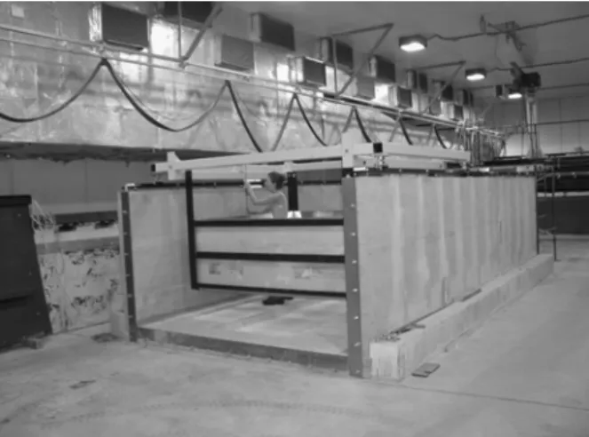
The test basin and the wagon assembly The test was set up in the CHC ice tank (Pratte and Timco 1981). The inside length and width of this basin was 6 and 2.6 m, respectively, with a height of 1.2 m (Fig. 2). The walls were 203 mm thick and were made of re-bar reinforced concrete. A

removable steel gate at one end of the basin was used to access the basin’s interior. Two sets of guide rails were anchored onto the top of the two longitudinal walls. These allowed motion of a frame assembly used to carry four containment walls, henceforth collectively referred to as wagon, into which ice growth was to take place and which was used to pull the ice block onto the sand.

Each wagon wall consisted of a 19 mm-thick plywood sheet 2 m in length and 0.79 m in width screwed onto the wagon’s structural members. A single 50 m long 800 watts heating cable was encased in a series of horizontal grooves in the plywood. The plywood sheets and the heating cable were covered with a thin sheet of stainless steel. The purpose of this set up was to deliver enough heat to the ice grown in the wagon to disengage it from the walls and allow it to slip downward onto the sand bed for testing. The sediment column

The sediments consisted of sand, which was obtained from a quarry in the Ottawa area. D10, D30 and D60 were 0.16, 0.30 and 0.61 mm, respectively, and the angle of repose was 32.5 degrees. It was laid on the floor of the basin, and compacted manually to a total thickness of 280 mm, about 75 mm below the wagon’s lowest structural member. This column included three 2-3 mm thick coloured sand layers at a distance of about 75, 155 and 215 mm from the

Figure 2: Test basin with enclosing wagon.

Step 1: Ice growth

Ice growth Water (20 ppt) Sand 2 m Insulation Load cells Wagon Pull rods Actuator

Step 2 : Lowering and vertical loading of ice

Ice loading with

concrete slabs Lowering of water level

Step 3 : Pulling of loaded ice sheet

Concrete

Position transducers

floor of the basin. These layers were used as markers, to help find out how much of the shearing occurred within the sand column as opposed to at the ice sand interface itself. Instrumentation

Two 45 kN capacity water-proofed load cell assemblies were mounted in parallel onto the downstream wagon wall (Fig. 1). They were located at the bottom of the wagon (as close as possible to the ice-sand interface) in order to minimize the amount of torque exerted onto the rail at the wagon’s suspension points. These cells monitored the load exerted onto the wagon by a steel bar connected to two stainless steel pull rods, which extended to and went through one of the basin’s end walls. Sealed guide tubes in the wall ensured water tightness. On the other side of that wall, the rods were clamped onto a second bar, itself driven by a worm gear actuator. Two gear ratios were available: 20:1 and 60:1. The actuator’s maximum travel distance was 124 mm, which was recorded by a position transducer. Position transducers were also used to monitor the vertical motion of the ice at midpoint along the four edges of the top concrete slab (Fig. 1). The voltage output from these seven channels (two load cells and five position transducers) was acquired at a rate of 100 Hz with a 30 Hz low-pass filter.

Procedures

A 20 ‰ saline solution was prepared in a large pit inside the CHC ice tank by diluting sodium chloride into tap water. Once the sand was laid out in the basin, enough of that water was transferred over to reach the wagon’s top rim (Step 1 in Fig. 1). The entire water surface outside the wagon was then covered with insulation and the cold room temperature was brought down to -15C. An air deflector was set up to orient the flow of cold air from the refrigeration vents onto the ice surface. An average thickness of 260 mm was achieved within several days, with a growth rate up to 6 mm per hour.

The heating cable inside the wagon walls was then activated while enough water was removed from the test basin so as to allow the ice block inside the wagon to drop onto the underlying sand bed (Step 2 in Fig. 1). It was found that, during this process, a significant amount of melting occurred along the four bottom edges of the ice block, such that these were rounded. This was not objectionable, however, since it reduced ‘edge effects’. In addition, before every test, the leading edge was probed manually and any sediment accumulation in front of the ice block was removed. Half way through the test program, the ice became too thin for testing to proceed so a second growth stage (up to 370 mm) was done. Such thinning either resulted from partial melting (the floor of the CHC ice tank is not insulated) or

abrasion.

The surface of the ice block was then covered with a 3 mm thick rubber foam and a 40 mm thick plywood board. These formed a base onto which a 470 kg concrete slab was laid. Once the four position transducers were installed on top of the slab, horizontal loading could proceed (Step 3 in Fig. 1). After test completion, the actuator was brought back to its initial position and another concrete slab was added to the vertical load for the next 124-mm test, and so on, up to a total mass of six tons. This corresponded to an upper bound stress on the seabed of about 15 kPa (taking into account all test parameters, as noted below).

TESTING

A total of 48 tests were conducted, divided into four series, each of which with increasing vertical load and at a given displacement rate. Another series was done with a constant load

but with displacement rates varying from one test to the next. Displacement rates ranged from 0.0025 to 0.3 mm/sec, at an ambient air temperature of - 4 ± 2o

C. The thickness and overall shape of the ice block was

monitored before and after each series (through holes drilled into the ice). Water level (for determining ice, board and concrete buoyancies) was also recorded. It ranged from 45 to 400 mm above the sand bed. Constants used throughout the test program for the calculation of the vertical load are water density (1019 kg/m3), ice density (estimated at 900 kg/m3) and wood panel volume and density. The net vertical load takes into account all these elements. The force required to slide the wagon assembly onto the rails with a floating ice block and at test temperature was about 200 N. It was subtracted from the horizontal loads measured during testing. On the onset of the test program, it was assumed that the relationship between vertical and horizontal loads would follow a Mohr-Coulomb type behaviour (Barker and Timco 2004), that is,

Ac F

F_H = _Vtanβ + (1)

where FH and FV are the horizontal and vertical loads, respectively, A is the area of the

ice/sand interface, c is the cohesion, tanβ is the friction coefficient and β is the friction angle (Fig. 3).

RESULTS The ice block

Prior to each test, the edges on the underside of the block were probed manually to check for ice shape and integrity. Doing so, a 'gap' was noted along the outside margins of the bottom

50 mm

Vertical Horizontal New growth

Top

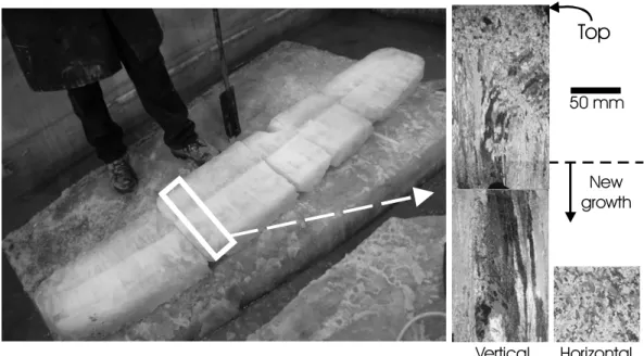
Figure 4: Cross-section of the ice block with vertical and horizontal (bottom surface) thin sections. Note the continuity in crystal structure resulting from the

new growth, a feature typical of 'congelation' ice.

Vertical Load (F )V Ho riz o nt a l L o a d (F )_H

Ac

β

surface, such that only about 70% of that surface was in actual contact with the sediments. (Since both the normal and the tangential loads are normalized over surface area, this reduction in effective footprint does not affect the results of our study.) When the ice was unloaded and allowed to float during the test program, visibility was too poor (due to the fine sediments in suspension) to allow a glance at the bottom surface with an underwater camera. However, up to three refrozen ice cracks a few millimetres in thickness running across the top surface of the block were observed later after unloading the ice. It is uncertain how this may have affected the ice-sand interaction.

At the end of the program, the water was removed from the test basin and the ice was sectioned with a chain saw (Fig. 4). At that time, it had a total thickness of 345 mm in the centre, thinning down to 260 mm along the margins, with a width of 1.96 m along all edges. The second (new) ice growth phase led to a conspicuous horizontal layering, shown in Fig. 4. The upper portion of the ice sheet was dominated with mm-sized crystals resembling frazil ice, which extended downward in a columnar structure. No sediments were incorporated into the ice, with the exception of the

lowermost 30 to 40 mm, where the ice was slightly brownish. Interestingly, the ice salinity was about 5 ‰ at the beginning of testing, but averaged 2 ‰ at the end, reflecting the temperature fluctuations the ice had undergone throughout the test program. Friction coefficients

Examples of load traces (the cumulative response of both load cells) are shown in Fig. 5 for a series of tests with increasing vertical load. These, and those for all other tests, display a similar pattern of strain softening: a regular increase in horizontal load with time (or

displacement) up to a peak, followed by a sudden drop and levelling off of the load. The peak load is that required to overcome static friction; the flat portion of the load trace is the result of the kinetic friction. When the latter segment was not perfectly flat, an average value was recorded. In some instances, the load trace at that stage comprised random (as shown by some of the traces in Fig. 5) or systematic cycling, thought to result from, respectively, slip

0 10 20 30 0 100 200 300 400 500 Time (seconds) kN Increasing vertical load

Figure 5: Horizontal load traces from one test series, for vertical loads ranging from 9 to 63 kN.

FH = 0.47FV + 1.6 FH = 0.39FV + 0.36 0 10 20 30 0 20 40 60 80 Vertical load (kN) Ho ri z o n ta l l o a d ( k N) STATIC KINETIC Linear (STATIC) Linear (KINETIC)

Figure 6: Linear behaviour of the

horizontal/vertical load ratio. The y-intercept (upon extrapolating) represents cohesion.

behaviour at the ice-sand interface and resonance of the wagon assembly. An average value for the horizontal load was also obtained in these cases. The slope of the initial load increase reflects the system stiffness. Early in the

experimental program, the pull rod bar at the actuator end was strengthened to reduce the amount of bending to an

acceptable level. This steepened the slope but did not otherwise affect the data. In all cases, a linear relationship was observed between the vertical loads and both the static and kinetic forces (Fig. 6), consistent with Coulomb-type friction behaviour. A linear regression allowed an estimate of both the slope and the y-axis intercept, the latter corresponding to the parameter Ac in Eq. 1. An average value of 1.5 and 1.4 kN for the y-intercept was derived

respectively for the static and kinetic response, corresponding to a cohesive stress of about 0.5 kPa.

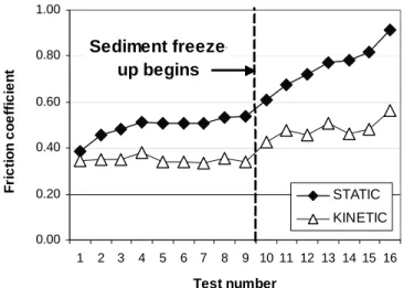
When the ice block was allowed to rest on the sand bed for a sufficient amount of time (a few days), the sediments' surface began to freeze. This is shown in Fig. 7 for the test series with various

displacement rates but where the vertical load remained constant. A substantial increase in friction is observed,

presumably related with the downward progress of the freezing front, and induced by

the interaction of frozen sand over unfrozen sand. Note that, in this figure, it is uncertain as to why the static friction coefficient increases slightly at the beginning of the test sequence. In Fig. 8, all the data are plotted as a function of displacement rate. A linear regression drawn for both sets of data does not display a significant trend (which remains within data scatter). The average value for these parameters, derived from tests in which the sediments were believed not to have been affected by freeze-up, is 0.47 (static) and 0.37 (kinetic) with a standard deviation of 0.03 in both cases.

tan β = 0.13R + 0.36 tan β = -0.04R + 0.47 0.00 0.10 0.20 0.30 0.40 0.50 0.60 0.001 0.01 0.1 1

Displacement rate (mm/sec)

Fr ic ti on c o e ff ic ie n t STATIC KINETIC Linear (KINETIC) Linear (STATIC)

Figure 8: Semi-logarithmic plot displaying the relationship between the friction coefficient (tan β ) and displacement

rate (R). 0.00 0.20 0.40 0.60 0.80 1.00 1 2 3 4 5 6 7 8 9 10 11 12 13 14 15 16 Test number F ri ct io n co ef fi ci en t STATIC KINETIC Sediment freeze-up begins

Figure 7: Variation in friction coefficient during one test series.

Vertical motion of the ice block

The readings from the vertical position transducers showed that the ice block always tended to sink into the sand column while traveling horizontally. This penetration, averaging 10 mm per test, was generally not uniform. During one test series, for instance, the block shifted about a horizontal axis oriented perpendicular to the travel direction. As a result, the leading edge of the ice block sank more than the opposite one. Since the wagon was pushed back to its starting position in the basin up to three times over the course of this test program, block sinking resulted in a slight downward slope in the sand bed in the travel direction (up to 2 degrees for the last series). Both the vertical and the horizontal load data were corrected accordingly.

Sand column

At the end of test program, the basin was drained and vertical pits were dug into the sand, in the direction of ice motion and perpendicular to it. No clear signs of shear (or tangential) stresses (such as overlapping sediment layers or a rotation component) were observed, suggesting that much of the horizontal displacement took place at the ice/sand interface. However, evidence for normal stresses was ubiquitous, in the form of compaction: the spacing between the coloured sand layers was locally reduced by up to 80%. This compaction could not be monitored during the tests but it is most likely linked with the sinking of the slab during its travel.

DISCUSSION

A number of studies have looked at the friction of ice against itself (Kennedy et al. 2000 and references therein) or various material (e.g. Barnes et al. 1971, Fiorio et al. 1997, Frederking and Barker 2002, amongst others). Few addressed the type of interaction relevant to the stability of an ice pad, that is, involving sea floor material. Shapiro and Metzner (1987) dragged two large blocks of sea ice up an unfrozen gravel beach with a bulldozer, yielding static and kinetic friction coefficients of 0.50 and 0.39 respectively. Takeuchi et al. (2003) investigated the friction between a thin sand layer and 95 mm diameter sea ice specimens, at displacement rates ranging from 3 to 20 mm/sec and with normal loads up to 450 kPa. They reported static and kinetic friction coefficients varying from 0.35 to 0.9 and 0.30 to 0.65, respectively, with temperature and the grain diameter as the most influential parameters. Friction resistance decreased slightly with an increase in displacement rates and with the addition of water to the sand specimen. In both of these studies, the interaction was assumed to be cohesionless (zero friction with no vertical load). Barker and Timco (2003) report a small decrease in kinetic friction with displacement velocities. The static friction obtained by Utt and Clark (1980) with small laboratory tests ranged from 0.85 to 1.47.

The experimental program described herein was aimed at simulating, in a laboratory environment, what is actually taking place in the field. There is no scaling involved. This is why the test basin was designed to accommodate an ice slab with such a large footprint. Moreover, the vertical stresses achieved are realistic: they corresponded to about 80% of those estimated from the Nipterk ice pad in the Beaufort Sea (Barker and Timco 2004). Given the linear behaviour of the force ratios, these results may be extrapolated to significantly higher stresses.

CONCLUSION

The salient results from this study are as follows: 1) The average static and kinetic friction coefficients are 0.47 (β = 25o) and 0.37 (β = 20o), respectively; 2) A Coulomb-type friction behaviour was observed, with an average cohesion force of 1.5 and 1.4 kN for the static and kinetic response, respectively, corresponding to a stress of about 0.5 kPa; 3) Friction

coefficients did not vary with displacement rates used in this test program; 4) Sediment freeze-up increased friction significantly; 5) Most of the horizontal displacement appears to have taken place at the ice/sand interface; and 6) The sediments record extensive evidence of normal shear, which is probably linked to the ice’s propensity to sink into the sand during its travel.

ACKNOWLEDGMENTS

This study was funded by the Program of Energy Research and Development (PERD) through the Northern Program at Objective Level (POL). Ed Funke of Comdor Engineering designed the experimental set-up. M. Sayed provided comments on an early version of the manuscript. REFERENCES

Barker, A. and Timco, G.W. (2003), “The friction coefficient of a large ice block on a sand/gravel beach”, 12th Workshop on the Hydraulics of Ice Covered Rivers, CGU HS Committee on River Ice Processes and the Environment, Edmonton, AB.

Barker, A. and Timco, G.W. (2004), “Sliding resistance of grounded spray ice islands.” Proc. 17th Symposium on Ice (IAHR 2004), St. Petersburg, Russia, pp. 208-216.

Barnes, P., Tabor, D. and Walker, J.C.F. (1971), “The friction and creep of polycrystalline ice.” Proc. Roy. Soc. Lond., A324, pp.127-155.

Frederking, R. and Barker, A. (2002), “Friction of sea ice on various construction materials.” Proc. 16th Symposium on Ice (IAHR 2002), Dunedin, New Zealand.

Fiorio, B., Meyssonnier, J. and Boulon, M. (1997), “Experimental study of the friction of ice over concrete at the centimetre scale.” Proc. 7th Int. Offshore Polar Engr. Conf. (ISOPE 1997), Honolulu, USA, pp. 466-472.

Kennedy, F.E., Schulson, E.M. and Jones, D.E. (2000), “The friction of ice on ice at low sliding velocities.” Phil. Mag. A., 80, pp.1093-1110.

Pratte, B.D. and Timco, G.W. (1981), “A new model basin for the testing of ice-structure interactions.” Proc. 6th Int. Conf. Port Ocean Eng. Arctic Cond. (POAC 1981), Vol. II, Quebec City, Canada, pp. 857-866.

Shapiro, L.H. and Metzner, R.C. (1987), “Coefficients of friction of sea ice on beach gravel.” J. Offshore Mech. Arctic Engrg., 109, pp. 388-390.

Takeuchi, T., Sasaki M., Miura, K., Sanbe, H., Takahashi, A. (2003), “Coefficients of friction of sea ice on sand”, Proc. 13th Int. Offshore Polar Engr. Conf. (ISOPE 2003), Honolulu, USA, pp. 461-464.

Utt, M.E. and Clark, R.A. (1980), “Coefficient of friction between submerged ice and soil”. Amer. Soc. Mech. Eng. Petroleum Division Journal, No.80-PET-41, p.1-4.