The Disk Wind in the Neutron Star
Low-mass X-Ray Binary GX 13+1
The MIT Faculty has made this article openly available. Please share
how this access benefits you. Your story matters.
Citation
Allen, Jessamyn L. et al. “The Disk Wind in the Neutron Star
Low-Mass X-Ray Binary GX 13+1.” The Astrophysical Journal 861, 1 (June
2018): 26 © 2018 The American Astronomical Society
As Published
http://dx.doi.org/10.3847/1538-4357/AAC2D1
Publisher
IOP Publishing
Version
Final published version
Citable link
http://hdl.handle.net/1721.1/120939
Terms of Use
Article is made available in accordance with the publisher's
policy and may be subject to US copyright law. Please refer to the
publisher's site for terms of use.
The Disk Wind in the Neutron Star Low-mass X-Ray Binary GX 13
+1
Jessamyn L. Allen1,2 , Norbert S. Schulz2, Jeroen Homan2,3 , Joseph Neilsen2 , Michael A. Nowak2 , and Deepto Chakrabarty1,2
1
Department of Physics, Massachusetts Institute of Technology, 77 Massachusetts Avenue, Cambridge, MA 02139, USA;[email protected] 2
Kavli Institute for Astrophysics & Space Research, MIT, 70 Vassar Street, Cambridge, MA 02139, USA 3
SRON, Netherlands Institute for Space Research, Sorbonnelaan 2, 3584 CA Utrecht, The Netherlands Received 2017 June 1; revised 2018 April 28; accepted 2018 May 5; published 2018 June 27
Abstract
We present the analysis of seven Chandra High Energy Transmission Grating Spectrometer and six simultaneous RXTE Proportional Counter Array observations of the persistent neutron star(NS) low-mass X-ray binary GX 13 +1 on its normal and horizontal branches. Across nearly 10 years, GX 13+1 is consistently found to be accreting at 50%–70% Eddington, and all observations exhibit multiple narrow, blueshifted absorption features, the signature of a disk wind, despite the association of normal and horizontal branches with jet activity. A single absorber with standard abundances cannot account for all seven major disk wind features, indicating multiple absorption zones may be present. Two or three absorbers can produce all of the absorption features at their observed broadened widths and reveal that multiple kinematic components produce the accretion disk wind signature. Assuming the most ionized absorber reflects the physical conditions closest to the NS, we estimate a wind launching radius of 7×1010cm, for an electron density of 1012cm−3. This is consistent with the Compton radius and also with a thermally driven wind. Because of the source’s high Eddington fraction, radiation pressure likely facilitates the wind launching.
Key words: accretion, accretion disks – stars: neutron – techniques: spectroscopic – X-rays: binaries – X-rays: individual(GX 13+1)
1. Introduction
Warm absorbers(partially ionized gas) are common to both black hole(BH) and neutron star (NS) low-mass X-ray binaries (LMXBs), identified through the narrow absorption features imprinted on the illuminating continuum. A group of warm absorbers have only been seen in sources with high inclina-tions, indicating the absorbing material is associated with the accretion disk. In all BH LMXBs and a subset of the NS binaries, the absorption features are blueshifted (Ponti et al. 2012, 2016; Díaz Trigo & Boirin 2013, 2016); the
absorbing material forms an outflow known as an accretion disk wind. When blueshifts are not present, the absorber is in a static configuration and is commonly called an accretion disk atmosphere. Warm absorbers were first observed in active galactic nuclei(AGNs) in the 1970s and later in X-ray binaries with the launch of ASCA in the 1990s(Ueda et al.1998; Kotani et al.2000). The high-resolution gratings onboard Chandra and
XMM subsequently revealed the complexity and ubiquity of the warm absorbers in LMXBs and, in the case of accretion disk winds, showed them to be a major component of the accretion picture(Neilsen et al.2011; Ponti et al.2012,2014).
The warm absorbers’ ionized resonance features are most often transitions in highly ionized species of iron, including the Kα line of FeXXV and FeXXVI, although some sources’ spectra exhibit over 90 absorption lines from transitions in dozens of ionized species, such as the BH binary GRO J1655−40 (Miller et al.2006; Kallman et al.2009). A single absorption zone
can often explain the absorption features, but in a number of sources, especially those with features other than iron lines, multiple absorption zones can more accurately reproduce the complex absorption signature. In the case of accretion disk winds, outflow speeds are typically in the range 300–1000 km s−1, although ultrafast outflows with velocities of 0.01–0.04c have been reported (Miller et al. 2015, 2016a, 2016b). As the
absorption features are only seen in high-inclination LMXBs (60° < i < 80° constrained by the presence of dips in light curves; Frank et al.1987) and no significant line re-emission is observed,
the absorbers are believed to have an equatorial geometry with a small opening angle or possibly a bipolar geometry with strong stratification in density and/or ionization above the accretion disk plane(Díaz Trigo & Boirin2013; Higginbottom & Proga2015).
In BH LMXBs there is a strong correlation between mass outflow and the accretion state. Accretion disk winds detected via blueshifted absorption features are found almost exclu-sively in soft spectral states, when the accretion disk is optically thick and the spectrum is disk-dominated (Ponti et al.2012).
Jets, detected via strong radio emission, are active in the hard spectral states, when the inner disk is believed to be optically thin and the spectrum has significant nonthermal emission. The blueshifted, narrow absorption features are also absent in hard states of high-inclination sources, suggesting the accretion disk wind is absent. There are, however, significant exceptions to the outflow–accretion state correlation; there is strong evidence that in at least five disk wind sources, including BH LMXB GRS 1915+105, winds and jets are simultaneous in luminous hard spectral states(Lee et al.2002; Homan et al.2016).
NSs may show a similar correlation between accretion state and outflow (Ponti et al.2014; Bianchi et al. 2017), but only
30% of high-inclination NS warm absorbers exhibit definite outflows (Díaz Trigo & Boirin2016). In addition, NS LMXB
outburst tracks are more varied than those of BHs (Muñoz-Darias et al.2014), and several NSs are included in the subset
of disk wind systems with possible simultaneous jets and winds (Homan et al. 2016). NS LMXBs are classified by their
behavior as atoll or Z sources, the latter being brighter (LX>0.5 LEdd) and less variable. In general, NSs are softer than BHs in outburst, in part due to the thermal boundary layer emission, but even NSs show significant variety in © 2018. The American Astronomical Society. All rights reserved.
spectral softness depending on their classification, with Z sources being much softer overall than atoll sources. These issues compound to make the outflow–spectral state correlation less obvious in NS LMXBs compared to BHs.
Radiation pressure, Compton heating, and magnetic forces can all launch outflows in accretion disk systems. In NS and BH LMXBs, the warm absorber plasmas are highly ionized, leaving too few transitions in the UV and the soft X-ray for line driving to be an effective wind launching mechanism(Proga & Kallman 2002). In a Compton-heated outflow,4 the accretion disk is strongly irradiated by the central X-ray-emitting region; beyond some point in the disk, the thermal velocity exceeds the local escape velocity, generating an outflow. Several BH LMXBs, including GRO J1655-40 and GRS 1915+105 (Miller et al.2006,2016b), have exhibited fast and/or dense outflows.
Magnetorotational instabilities or magnetocentrifugal forces can launch winds very close to the central compact object, which can account for the high wind densities and large blueshifts. There is also the possibility that different wind driving mechanisms are active at the same time but dominate in different spectral states and/or luminosities (Neilsen & Homan 2012; Homan et al. 2016), due to a hybrid wind
driving mechanism. For the brightest disk wind sources accreting at near-Eddington rates, radiation pressure on electrons should increasingly contribute to the wind driving in addition to the dominant mechanism (Proga & Kallman
2002; Homan et al. 2016; Done et al. 2018; Tomaru et al.2018).
Determining disk wind launching mechanisms and spectral state dependence have powerful implications beyond under-standing disk wind properties. While disk winds are relatively slow outflows (v0.01c), they can carry significant mass away from the binary, comparable to the accretion rate. High mass-loss rates can create accretion disk instabilities which may produce luminosity modulations or instabilities that may drive state transitions (Begelman & McKee 1983; Shields et al.1986), and may also be significant enough to alter binary
and spin evolution timescales (Ponti et al.2012). A complete
picture of outflows in stellar mass compact object systems will help to understand accretion on much larger mass scales, including supermassive BHs in AGNs which also exhibit powerful jets and winds.
1.1. NS LMXB GX 13+1
The NS LMXB GX 13+1 (also known as 4U 1811−171) is a bright, persistent accretor located in the Galactic bulge. It orbits an evolved late-type K5 III star (Fleischman 1985; Bandyopadhyay et al. 1999) and has an estimated distance of
7± 1 kpc (Bandyopadhyay et al.1999). Studies of infrared and
X-ray light curve modulations (Corbet et al. 2010; Iaria et al.2014) as well as X-ray dips (D’Aì et al.2014), support a
binary orbital period of 24.7 days and a highly inclined orbit (60°–80°; Díaz Trigo et al.2012).
Originally classified as an atoll source (Hasinger & van der Klis1989), GX 13+1 was later re-classified as a Z source due
to strong secular evolution of its color–color and hardness– intensity diagrams(CDs and HIDs), rapid movement along its CD & HID tracks, and variability levels, all behaviors
consistent with other well-established Z sources (Homan et al.1998; Fridriksson et al.2015).
A warm absorber in GX 13+1 was first discovered by Ueda et al.(2001), made evident by an iron Kα absorption line in GX
13+1ʼs ASCA spectrum. Subsequent Chandra and XMM observations revealed a more detailed picture of the ionized material’s properties via its absorption imprinted on GX 13 +1ʼs spectrum. Analyzing a set of XMM-Newton European Photon Imaging Camera (EPIC) observations, Sidoli et al. (2002) reported Kα and Kβ absorption lines of FeXXV and FeXXVI, along with a Kα CaXX line. Despite large velocity shifts detected in several absorption features (−3000 to −5000 km s−1), blueshifts were not detected in all absorption lines and the errors on the outflow velocity were large (±2200 km s−1). A Chandra High Energy Transmission Grating Spectrometer (HETGS) observation in 2001 of GX 13+1 revealed the Kα lines from H-like Fe, Mn, Cr, Ca, Ar, S, Si, and Mg as well as He-like Fe (Ueda et al. 2004). The
absorption lines shared a common blueshift of ≈460 km s−1, corresponding to an outflow velocity of ≈400 km s−1 when corrected for proper motion. The inferred mass outflow rate of the disk wind was determined to be comparable to the accretion rate (≈1018 g s−1), indicating disk winds are a significant component of the accretion process in GX 13+1.
Ueda et al. (2004) favored a radiation-driven outflow that
develops at sub-Eddington luminosities for the accretion disk wind in GX 13+1. In later XMM RGS observations of GX 13+1 Díaz Trigo et al. (2012) found strong correlations
between the hard flux and the warm absorber’s properties (column density and ionization), concluding the absorber was consistent with a Compton-heated disk wind.
Madej et al.(2014) analyzed all available Chandra gratings
observations of GX 13+1 in an attempt to measure orbital parameters using the disk wind, but were hindered by the intrinsic variability of the source and the wind. In this paper we present a re-analysis of the same set of archived Chandra HETGS observations with the primary goal of understanding the evolution of this wind. We perform detailed absorption line fitting and utilize RXTE data to track the disk wind properties throughout the system’s CD. In contrast to previous studies that assumed a single absorber, we find that the disk wind must comprise multiple absorption zones.
2. Observations
In our study of GX 13+1ʼs accretion disk wind, we utilize a data set of seven Chandra HETGS observations, six of which have simultaneous RXTE/Proportional Counter Array (PCA) coverage. The details are listed in Table1.
2.1. Chandra Observations
We have analyzed all seven Chandra HETGS (Canizares et al.2005) observations of GX 13+1, for a total exposure of
approximately 190 ks. The observations span 10 years, with five of the observations taken during a two week timespan in 2010 July and August. Observations were taken in both timed exposure(TE) and continuous clocking (CC) modes with the Advance CCD Imaging Spectrometer S-array (ACIS-S). For TE mode observations, a 350-row subarray was used, yielding a 1.24 s frame time. In CC mode, spatial information was collapsed into 1 row, reducing the frame time to 2.85 ms. 4
While Compton-heated winds are often called“thermally driven” winds, we will use“Compton-heated winds,” or simply “Compton winds” to be explicit about the heating mechanism.
2
The Chandra data were downloaded from the Chandra Data Archive5 and re-processed using the TGCat (Huenemoerder et al. 2011) run_pipe script with CIAO 4.9 (Fruscione
et al. 2006) and CALDB 4.5.0 in ISIS6 version 1.6.2–30 (Houck et al. 2013). Our GX 13+1 HETGS data processed
with CIAO 4.9 differ slightly from data processed with older versions of CIAO due to changes in the correction for contaminant build-up on Chandra’s optical blocking filter. The most significant deviations approach the 10% level at long wavelengths (>8 Å) for both the High Energy Grating (HEG) and Medium Energy Grating(MEG) first orders.
The zero-order position determines the absolute accuracy of the wavelength measurements. As GX 13+1ʼs zeroth order is significantly piled-up in TE mode observations, we cannot use a centroid calculation due to the distorted point-spread function. We used findzo to calculate the zero-order position from the intersection of the MEG spectrum and the ACIS frame-shift streak, which provides a zero-order position accuracy of less than 0.1 ACIS-S detector pixels, corresp-onding to 0.001Åfor the HEG and MEG first orders. First-order redistribution matrix files and ancillary response files were created with the run_pipe script.
D’Aì et al. (2014) reported a dipping event approximately
halfway through ObsID 11814. Dips have been associated with spectral changes in both the warm absorber and neutral absorption column (Díaz Trigo et al.2006). We removed the
dip event, including the ingress and egress of the event based on times reported by D’Aì et al. (2014) and performed spectral
analysis only on the non-dipping spectrum.
We used the AGLC script7in ISIS to create the ACIS-S grating light curves and compute hardness ratios. Hardness ratios are defined as the number of hard counts (3–8 keV) divided by the number of soft counts (0.5–3 keV). The count rate varied on the level of 15%, but we found no significant changes in the source’s intensity or spectral hardness, so we analyzed observations whole, except for ObsID 11814 as stated above.
2.2. RXTE Observations
We also analyzed data from the RXTE PCA (Jahoda et al.
2006). For a list of the individual RXTE/PCA observations that
were performed simultaneously with our Chandra observations we refer to Table 1 in Homan et al. (2016). As the RXTE
continuum parameters did not vary significantly between orbits, we summed the individual orbit eventfiles using the sumpha tool to produce a single RXTE spectrum for each corresponding Chandra HETGS observation.
For our X-ray CDs of GX 13+1, we made use of RXTE/ PCA data published in Fridriksson et al. (2015). We refer to
that paper for the details of the data reduction. GX 13+1 exhibits significant secular motion of its Z track on the timescales of days or longer. Fridriksson et al.(2015) organized
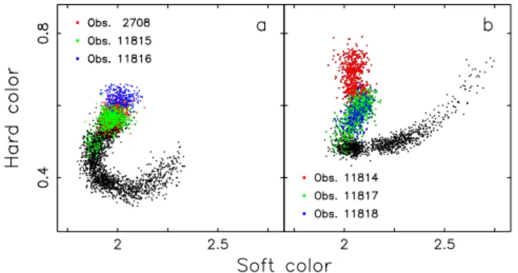
the source’s RXTE data into six different CD tracks. Correlating the source’s RXTE position on the Z tracks during our Chandra HETGS observations, see Figure1, ObsIDs 2708, 11815, and 11816 fall on one Z track that has less distinct branches (Homan et al. 2016), while GX 13+1 moved along the
horizontal branch(HB) and normal branch (NB) on another Z track during ObsIDs 11814, 11817, and 11818.
3. Analysis and Results
All spectral analysis was performed withinISIS. Errors on fit parameters were calculated with conf_loop and correspond to the 90% confidence bounds (σ = 1.6, Δχ2= 2.71). All quoted chi-squared values, cn2 (dof), are reduced. We used the calc_flux ISIS tool to calculate (absorbed) fluxes and (unabsorbed) luminosities. The 0.5–10 keV and bolometric (0.1–100 keV) luminosities were calculated assuming a dis-tance of 7 kpc. The Eddington fraction (LX/LEdd= fEdd) assumed an Eddington luminosity, LEdd, of 2×1038erg s−1 for a 1.4 MeNS with a hydrogen-rich photosphere.
We fit the uncombined HEG and MEG ± 1 orders with matched spectral grids across the 1.65–9.5 Å (1.3–7.5 keV) range, corresponding to a resolution of 0.023Å across our energy band. Each bin contained a minimum of 20 counts which allowed us to useχ2statistics.
While the HEG has twice the spectral resolution as the MEG and experiences less pile-up, our spectral analysis benefited from the additional MEG counts. Continuum and Table 1
Chandra HETGS and RXTE PCA Observation Details
Date Chandra HETGS RXTE PCA
ObsID Mode Exposure(ks) Count Rate(s−1)a Exposure(ks) Count Rate(s−1) RXTE Color Diagram Positionb
2002 Oct 8 2708 TE 29.4 13.5 9.8 16.7 Upper NB→ NB/HB vertex
2010 Jul 24 11815 TE 28.1 13.9 13.2 16.7 Mid NB→ Upper NB
2010 Jul 30 11816 TE 28.1 13.6 5.7 16.1 Lower HB→ Upper NB
2010 Aug 1 11814 TE 26.8/28.1c 11.2/11.1 9.1d 17.0 NB/HB vertex → upper HB
2010 Aug 3 11817 TE 28.1 13.0 10.3 16.4 NB/HB vertex → NB/FB vertex
2010 Aug 5 11818 CC 23.0 14.6 5.2 15.8 Lower NB→ NB/HB vertex
2011 Feb 17 13197 CC 10.1 17.9 L L L
Notes.
aThe Chandra0.5–10 keV count rate and the RXTE3–40 keV count rate. b
NB= Normal Branch, HB = Horizontal Branch, FB = Flaring Branch. c
Observation details whenfiltered/unfiltered for the dip event. d
The RXTE observation did not cover the dipping event and, hence, was notfiltered.
5
http://cxc.harvard.edu/cda/ 6 http://space.mit.edu/cxc/isis/ 7
line parameters were better constrained when both HEG and MEG first orders (±1) were used.8ObsID 13197 was a CC mode calibration observation; two arms (MEG −1 and HEG +1) fell off the CCD, leaving only the MEG +1 and HEG−1 orders.
For the RXTE/PCA data, the background subtracted spectra were extracted from the Proportional Counter Unit 2 and a systematic error of 0.6% was added. Bins between 3 and 40 keV were noticed in the continuumfits.
3.1. Continuum Fitting
3.1.1. Pile-up
As GX 13+1 is bright (≈0.2 Crab) and five of the seven observations were taken in TE mode, spectra can suffer from significant pile-up. Pile-up has effects of energy and event grade migration that reduce the total source count rate and distort the observed spectral shape.9 We used the ISIS convolution model simple_gpile2 to quantify and mitigate the pile-up effects(Nowak et al.2008; Hanke et al.2009). The TE
mode observations experienced maximum pile-up at 3Å (≈4.1 keV).
In addition to generating spectral distortion, pile-up has the effect of reducing an absorption feature’s measured equivalent width (EW). The local pile-up fraction is proportional to the local count rate, which means that the local continuum is more suppressed relative to the absorption feature, reducing the observed EW. Our attempt to correct the EWs due to pile-up suppression is outlined in Section 3.2.
While the CC mode observations have a significantly shorter frame time making pile-up essentially negligible, they do not help us quantify the pile-up effects on the continua of the TE mode observations due to contamination by an X-ray scattering halo. GX 13+1 is highly absorbed and the CC mode continua include the dispersed scattering halo, which is difficult to model.
3.1.2. ISM Absorption
The neutral absorption column toward GX 13+1 is known to be large, with published values in the range of NH= (3–5)×1022cm−2(NH,22= 3–5; Ueda et al.2001; Díaz Trigo et al.2012; Schulz et al.2016). We used the absorption
model tbnew v2.3, with the abundances set to those of Wilms et al.(2000) and the cross-sections set to Verner et al. (1996).
In our joint fits of the Chandra HETGS and RXTE/PCA data, we found that the cn2was improved when we allowed the column density to vary between the two data sets. The Chandra HETGS data were well-fit with column densities in the range of NH,22= 4.9–5.0, while for the RXTE/PCA data, NH,22= 3.5–3.9. The Chandra HETGS column density was consistently≈30% higher than that of RXTE/PCA and is likely associated with the X-ray scattering halo. Chandra’s field of view is narrow relative to RXTEʼs and, thus, the Chandra HETGS observations do not include the X-ray scattering halo, while the RXTE/PCA observations do. The scattered X-rays from the halo are an additional source of low-energyflux in the RXTE spectrum, which can be modeled, tofirst order, with a lower neutral column density. We leave a more complete investigation of the X-ray scattering halo’s effects on the joint analysis of Chandra and RXTE data to a future paper.
We also found that the cn2value was always improved when the silicon abundance of the HETGS tbnew component was allowed to vary, yielding silicon overabundances between 2.0 and 2.1. The required silicon abundance is due to tbnewʼs incomplete modeling of the Si K edge (Schulz et al. 2016).
Additional structure in the Si K-edge, i.e., the near and far edge absorption, is apparent, including a line at 1.865 keV likely associated with a moderately ionized plasma in GX 13+1. We did not attempt to model the silicon edge beyond allowing for the overabundance in tbnew.
3.1.3. Continuum Models
When fit by itself, the GX 13+1 Chandra HETGS continuum was consistent with multiple model prescriptions as the large interstellar medium(ISM) absorption (NH,22>1) reduces the soft X-ray sensitivity and limits our ability to distinguish between continuum models. We found the diskbb +bbodyrad and bbodyrad+powerlaw continuum models, the most common models for NS LMXBs accreting at high rates, performed equally well.
Joint fits of the HETGS and PCA spectrum required three major spectral components; wefit a diskbb+bbodyrad+power-law model to the broadband continuum. Both the HETGS and PCA spectra were modified by neutral absorption columns with variable column densities. The HETGS continuum also included the pile-up convolution model simple_gpile2 and seven narrow absorption features modeled with negative Gaussians(see Section3.2).
The PCA spectrum was modified by two edge components: one with afixed energy (8.83 keV) and another left free to vary, yielding an average fit value of 7.1 keV. Both edges were required to obtain good cn2values for ourfits of the RXTE data. The edge at 8.83 keV is unresolved in the PCA spectrum but is seen in the XMM GX 13+1 spectrum (Díaz Trigo et al.2012),
while the edge at 7.1 keV is likely a superposition of narrow iron absorption features and a broad iron emission line. Details of fitting a broad emission line to the Chandra data are in Section3.1.4.
Figure 1. Two of GX 13+1ʼs Z track CDs with the color-coded points corresponding to six of the Chandra observations that occurred simultaneously with RXTE monitoring. In several observations, including ObsID 11816, the source only moved slightly along the Z track during the course of the observation(from the lower HB to the upper NB), while in ObsID 11817 the source moved along the entire horizontal branch, from the NB/HB vertex to the NB/FB vertex.
8
The only exceptions are the FeXXVIand FeXXVabsorption lines and the broad iron emission line, for which we excluded the MEG due to its low effective area at 7 keV.
9
http://cxc.harvard.edu/ciao/download/doc/pileup_abc.pdf
4
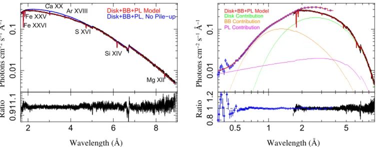
The continuumfit to the TE mode observations is shown in Figure 2 and the continuum parameters can be found in Table 2. In our continuum prescription, the multicolor disk component is the accretion disk while the blackbody comp-onent is likely boundary layer emission from the NS. Both the blackbody and disk components exhibit slight variations in their temperatures and normalizations, but there is no clear correlation among the parameters or the sourceflux, likely due to the large neutral column which introduces degeneracies in our continuum fits. The 0.5–10 keV absorption-corrected luminosity varies on the order of 10% across all observations, LX≈(7.3–8.6)×1037erg s−1.
3.1.4. Broad Iron Emission Line
Broad iron emission lines are common to both BH and NS LMXBs(White et al.1986; Asai et al. 2000). In NS binaries,
possible origins include the inner accretion disk, an accretion disk corona, and an ionized accretion disk wind, with the line being broadened by relativistic, Compton scattering and electron down-scattering mechanisms, respectively.
A broad iron emission line has previously been seen in the spectra of GX 13+1 with multiple X-ray instruments including ASCA, XMM/EPIC, RXTE/PCA and Chandra HETGS (Asai et al. 2000; Ueda et al. 2001, 2004; Sidoli et al. 2002; Díaz Trigo et al. 2012; D’Aì et al. 2014). Although nearby
Fe Kα absorption features make it difficult to constrain the emission line’s parameters, its energy and EW have been found to be variable. A 1994 ASCA observation revealed an emission line with energy 6.42± 0.08 keV, σ<220 eV, and EW= 19 ± 8 eV (Asai et al.2000; Ueda et al.2001), while in
XMM observations the emission line had higher energies (6.5–6.8 keV) and significantly larger widths (σ = 0.7–0.9 keV) and EWs (100–200 eV) (Sidoli et al. 2002; Díaz Trigo et al. 2012). The correlation between the iron emission and
absorption line EWs suggested a common origin in the outer disk(i.e., an accretion disk wind; Díaz Trigo et al.2012).
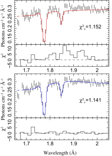
The Chandra HETGS data are well fit in the 6–7 keV (≈1.8–2 Å) range with two narrow absorption features corresponding to the Kα transitions of FeXXV and FeXXVI
(See Section3.2), but an excess of positive residuals is apparent
(see the top panel of Figure3). The RXTE/PCA data cannot
resolve the narrow iron absorption features but require an “edge-like” feature at 7.1 keV; this feature does not appear as an edge in the Chandra or XMM data.
The best jointfit to the Chandra and RXTE data is achieved when a broad emission line is added to the Chandra continuum model, along with the two narrow absorption features, while only an edge isfit to the RXTE data. The improved fit to the Chandra data with the emission line is shown in the bottom panel of Figure3.
We allowed the RXTE/PCA edge energy to vary even thoughfixing the edge energy did not affect the quality of the fits. Simply fitting two narrow absorption features and a broad emission line to both the Chandra and RXTE did not work, implying there is additional absorption outside our Chandra band that is unresolved with RXTE. Díaz Trigo et al. (2012)
reported additional narrow iron absorption features at 7.91 and 8.24 keV.
The broad emission line’s properties are listed in Table3. We found the broad line had typically energies of 6.48–6.60 keV (1.88–1.91 Å), σ = 0.18–0.29 keV, and EWs of 20–40 eV, more consistent with the emission line properties when observed with ASCA(Asai et al.2000; Ueda et al.2001) than with XMM/EPIC
even considering the large XMM error bounds(Díaz Trigo et al.
2012). We see a weak correlation between the broad emission
feature’s EW and the source’s hard flux which has also been seen in XMM/EPIC data of GX 13+1; the broad emission line’s EW is smallest(largest) in 11814 (11816), when the source is at its faintest(brightest) luminosity in this set of observations. We do not, however, observe the correlation between the narrow iron absorption features’ EWs and the broad emission line’s EW reported by Díaz Trigo et al.(2012).
3.2. Narrow Line Fits
We focused on known absorption features in GX 13+1ʼs spectrum, i.e., those identified by Ueda et al. (2004). We
combined all HEG and MEG m= ±1 orders using the ISIS combine_data sets function. Using a power law tofit the local Figure 2.Left: combined HEG and MEG± 1 orders for all five TE mode observations (data plotted in black) fit with a disk plus blackbody continuum and Gaussian absorption features(shown in red). The continuum model without simple_gpile2, plotted in blue, shows how the spectrum would appear without pile-up. Additional structure in the silicon edge is seen in the residuals near 6.6Å. Right: continuum fit to the combined TE mode observations (black) along with the combined RXTE/PCA observations (blue). The disk, blackbody, and power-law contributions are plotted in green, orange, and purple, respectively.
Table 2
Parameters for DiskBB+BB+PL Continuum Model
ObsID NH,22(1)a Si(1)b NH,22(2)c BB kT BB normd Disk Tin Disk Normd PL norme β β F0.5–10(BB)f F8–10g L0.5–10h fEddi cn2(dof)
(keV) (km2) (keV) (km2) ±1 MEG ±1 HEG
2708 4.88± 0.04 2.1± 0.1 3.87± 0.27 2.61± 0.09 1.5± 0.3 1.75± 0.02 94± 4 0.31± 0.10 0.031/0.031 0.017/0.020 6.93(0.10) 0.90 8.18 0.45 1.156(6047) 11815 4.97± 0.03 2.1± 0.1 3.59± 0.25 2.36± 0.09 2.2± 0.6 1.69± 0.02 105± 5 0.51± 0.06 0.025/0.026 0.017/0.017 7.02(0.11) 0.87 8.55 0.45 1.137(5975) 11816 4.91± 0.04 2.1± 0.1 3.50± 0.26 2.48± 0.08 2.6± 0.6 1.72± 0.03 95± 5 0.46± 0.10 0.026/0.028 0.019/0.019 7.07(0.15) 0.96 8.35 0.45 1.141(5939) 11814 4.99± 0.03 2.0± 0.1 3.48± 0.26 2.45± 0.07 3.1± 0.5 1.70± 0.03 76± 4 0.62± 0.09 0.029/0.030 0.024/0.023 6.02(0.20) 0.88 7.25 0.38 1.123(5831) 11817 5.00± 0.03 2.0± 0.1 3.55± 0.25 2.57± 0.08 1.4± 0.3 1.82± 0.02 77± 1 0.36± 0.08 0.027/0.028 0.019/0.019 6.81(0.09) 0.91 7.93 0.43 1.134(5883) Notes. a
Chandra HETGS column density. b
Allowing for a silicon overabundance in Chandra HETGS tbnew component improved the Si K edgefit. c
RXTE/PCA column density. d
The emission areas of the thermal components were calculated assuming a distance of d= 7 kpc. For the disk component, we additionally assumed an inclination of i = 70°. e
The power-law normalization. The power-law photon index,Γ, is fixed to 2.5 in all fits. f
The 0.5–10 keV Chandra HETGS flux in units of 10−9erg s−1cm−2with the blackbody fraction in parentheses. g
The 8–10 keV Chandra HETGS flux in units of 10−9erg s−1cm−2. h
The 0.5–10 keV Chandra HETGS luminosity with units 1037erg s−1(assuming d = 7 kpc).
iThe Eddington fraction calculated from the 0.1–100 keV RXTE/PCA unabsorbed flux; the power-law flux is excluded below the blackbody temperature.
6 The Astrophysical Journal, 861:26 (17pp ), 2018 July 1 Allen et al.
continuum within±1 Å of the line center, we fit a Gaussian function to the absorption feature ignoring nearby absorption features and edges. Line shifts, turbulent velocities (computed from the Gaussian FWHM) and EWs were calculated for each absorption feature in each observation.
As previously mentioned in Section 3.1.1, pile-up reduces the measured EW. To estimate the pile-up suppression, we calculated each absorption line’s EW with and without the simple_gpile2 pile-up component evaluated in our broadband continuum model. The ratio of the the EWs without and with the pile-up model was a multiplicative correction factor to the EW calculated with the method outlined in the previous
paragraph, which provided the best local continuum fit and, hence, the best measure of the EW. As visible in Figure 2, pile-up is most severe near 3Å, agreeing with our correction factors which were largest for the CaXX and ArXVIII EWs (approximately 10% and 5% respectively) at 3.01 and 3.73 Å. For the other absorption features, the EWs were suppressed by less than 5%. The EWs in Table 4 and Figure 4 have been corrected for pile-up.
Our Gaussian line parameters are shown in Table 4. The Kα transitions of FeXXVI, FeXXV, CaXX, SXVI, SiXIV
and MgXII were detected in all of the Chandra HETGS Figure 3.ObsID 11816, MEG and HEG±1 orders. Top: when only the local
FeXXVIand FeXXVabsorption features arefit, there is an excess of positive residuals in the 1.8–2.0 Å range. The residuals have been heavily binned to make the residual pattern more apparent. Bottom: adding an emission line centered at 1.88Å (6.60 keV, indicated by the dashed vertical line) improves thefit.
Table 3
Broad Fe Emission Gauss Parameters
ObsID EC σ Norm EW
(keV) (keV) (10−3ph s−1cm−2) (eV)
2708 6.58± 0.13 0.29± 0.15 2.27± 1.12 29± 14 11815 6.54± 0.08 0.21± 0.07 2.26± 0.80 28± 10 11816 6.60± 0.07 0.25± 0.08 3.05± 0.98 38± 12 11814 6.53± 0.09 0.18± 0.10 1.49± 0.68 21± 10 11817 6.48± 0.10 0.26± 0.11 2.30± 0.86 28± 11 Table 4 Gauss Line Parameters
ObsID Line vout vturb EW
(km s−1) (km s−1) (eV) 2708 Fe-XXVI 610± 80 1210± 150 48.0± 5.0 Fe-XXV 860± 160 1250± 280 24.0± 5.0 Ca-XX 550± 140 410± 210 2.9± 0.8 Ar-XVIII 440± 180 210± 100 1.2± 0.6 S-XVI 480± 70 450± 140 2.9± 0.6 Si-XIV 490± 50 460± 90 2.6± 0.3 Mg-XII 310± 160 600± 260 1.6± 0.8 11815 Fe-XXVI 740± 80 1050± 150 44.0± 4.0 Fe-XXV 980± 140 1220± 240 26.0± 4.0 Ca-XX 550± 160 100± 50 2.5± 0.7 Ar-XVIII 620± 200 300± 150 1.3± 0.7 S-XVI 610± 110 590± 230 2.6± 0.6 Si-XIV 590± 60 540± 110 2.6± 0.4 Mg-XII 560± 120 370± 180 1.1± 0.7 11816 Fe-XXVI 930± 100 1200± 170 41.0± 4.0 Fe-XXV 1210± 70 50± 20 11.0± 3.0 Ca-XX 450± 750 800± 400 1.5± 0.9 Ar-XVIII 530± 280 370± 180 1.0± 0.7 S-XVI 880± 230 30± 10 1.1± 0.6 Si-XIV 670± 80 230± 120 1.3± 0.3 Mg-XII 80± 900 810± 410 0.7± 3.0 11814 Fe-XXVI 730± 130 1140± 240 34.0± 5.0 Fe-XXV 930± 220 320± 160 11.0± 4.0 Ca-XX 830± 370 390± 190 1.5± 0.8 S-XVI 390± 160 440± 220 1.7± 0.7 Si-XIV 270± 80 530± 140 2.2± 0.5 Mg-XII 280± 290 540± 270 1.0± 1.0 11817 Fe-XXVI 500± 90 810± 180 34.0± 4.0 Fe-XXV 590± 230 1240± 380 17.0± 5.0 Ca-XX 560± 290 200± 100 1.4± 0.7 Ar-XVIII 280± 360 450± 220 1.2± 0.7 S-XVI 390± 100 110± 50 1.9± 0.5 Si-XIV 380± 50 330± 100 2.2± 0.3 Mg-XII 320± 100 50± 20 0.8± 0.5 11818 Fe-XXVI 390± 100 530± 270 31.0± 3.0 Fe-XXV 810± 210 700± 350 15.0± 3.0 Ca-XX 430± 310 840± 420 2.9± 1.0 Ar-XVIII 690± 380 110± 50 0.6± 0.3 S-XVI 370± 150 210± 100 1.6± 0.6 Si-XIV 340± 80 230± 120 1.4± 0.4 Mg-XII 330± 210 210± 110 0.6± 0.3 13197 Fe-XXVI 870± 200 1210± 460 40.0± 7.0 Fe-XXV 880± 220 1280± 440 33.0± 6.0 Ca-XX 630± 280 620± 310 4.0± 2.0 Ar-XVIII 370± 250 640± 320 2.8± 1.0 S-XVI 450± 160 470± 240 3.1± 1.0 Si-XIV 560± 90 570± 140 3.5± 0.6 Mg-XII 240± 320 570± 290 2.0± 1.0
observations. The Kα ArXVIIIis absent in ObsID 11814. The abundance of absorption features in the GX 13+1 spectra is in contrast to the XMM observations analyzed in Díaz Trigo et al. (2012), where the only disk wind absorption features present
were the the Kα and Kβ transitions of FeXXVI and FeXXV. The Chandra HETGS observations lack the signal-to-noise ratio (S/N) above 8 keV to study the iron Kβ transitions, if present.
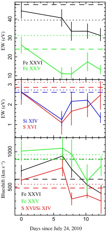
The FeXXVI, FeXXV, SXVI, and SiXIVEWs across the two week observation period in 2010 July and August are shown in the top and middle panels of Figure4. The solid dashed lines indicate the line’s EW in the 2001 observation (ObsID 2708) and the dotted line shows the line’s EW in 2011 (ObsID 13197). Despite the observations occurring almost eight years apart, ObsID 2708 (2002 October) and ObsID 11815 (2010 July) exhibit all four major absorption features with almost identical EWs.
There is no clear timescale of variability, but there are significant changes in the absorption features’ properties between observations, which occur, at minimum, approxi-mately two days apart. Between ObsIDs 11815 and 11816, separated by six days, the FeXXV, SXVI, and SiXIVEWs all decrease by factors of ≈2 while the FeXXVI EW is relatively constant. If all of the absorption features are produced by a single absorption zone, this trend in the EWs requires two simultaneous changes in the accretion disk wind: an increase in the plasma’s ionization state along with a decrease in the column density; this would allow the FeXXVI
line EW to remain constant while producing a decrease in the SXVI, SiXIV, and FeXXV EWs. Alternatively, if the FeXXVI
absorption feature is produced by a different absorber than the lower ionization absorption features, a decrease in the column density of the respective absorbing region could produce the observed decrease in the SXVI, SiXIV,and FeXXVEWs while not necessarily producing any significant change in the FeXXVIEW.
We compared the blueshifts of the FeXXVand FeXXVIlines with an average of the SXVI and SiXIV line shifts, shown in the bottom panel of Figure4. The iron lines appear to exhibit larger blueshifts (500–1200 km s−1) and turbulent velocities (1000 km s−1) than absorption features with lower ionization energies, including SXVIand SiXIV(with vout≈300–600 km s−1 and vturb≈300–550 km s−1). This trend may be related to the decreasing spectral resolution at lower wavelengths in the iron region or may indicate distinct absorption zones with different outflow velocities in the disk wind. Additionally, the FeXXV
line exhibits a consistently higher blueshift than the FeXXVIline, which could indicate that multiple kinematic components produce the iron absorption features. However, the error bounds on the velocities prevent us from claiming the existence of two or more kinematic components. We do see systematic changes in the outflowing plasma’s blueshift between observations, as previously reported by Madej et al.(2014). The average blueshift between the
two sets of lines increases from ≈675 to ≈850 km s−1between July 24 and 30 (ObsIDs 11815 and 11816) while the average blueshift decreases to≈350 km s−1six days later(ObsID 11818).
3.2.1. Manganese and Chromium Lines
In the 2001 Chandra observation of GX 13+1 (ObsID 2708), Ueda et al. (2004) reported MnXXV and CrXXIV
absorption with EWs of 3.6 and 4.1 eV, respectively. In our analysis of ObsID 2708, we were able tofit absorption features with EWs of 3.5±0.9 and 3.4-+1.6
0.9
eV but we consider the manganese line consistent with noise. As ObsID 2708 exhibits similar continuum parameters andfluxes as the other observa-tions, we combined all TE mode HEG±1 orders to increase Figure 4.Top and middle: equivalent widths(EWs) of the FeXXVI(black),
FeXXV (green), SXVI (red), and SiXIV (blue) absorption features in the observations spanning two weeks in 2010 July–August (ObsIDs 11815, 11816, 11814, 11817, and 11818). The long-dashed lines show each absorption line’s EW in the 2001 observation (ObsID 2708); the dotted lines indicate values measured in the 2011 observation (ObsID 13197). Bottom: line blueshifts calculated from Gaussian fits to the FeXXVI (black) and FeXXV (green) absorption lines and an average blueshift of the SXVIand SiXIVlines(red). There is evidence of an offset between the faster iron lines and the slower silicon and sulfur lines, as well as an offset between the FeXXVIand FeXXV lines.
8
the S/N in the 1.9–2.1 Å band, see Figure 5. No MnXXV
absorption is present, while a possible narrow (σ<0.005 Å) CrXXIV line is observed at 2.088Å; the line energy corresponds to a blueshift of≈700 km s−1, which is consistent with the blueshifts we observed in the individual TE mode observations(500–1000 km s−1).
3.3. Photoionization Model
In essentially all LMXB disk winds, the absorbers have temperatures below the threshold of a collisionally ionized plasma (kB Te≈EI, where Te is the electron temperature, EI is the ionization energy of the plasma ions). In our Chandra HETGS spectra, we modeled the absorption line features with the photoionized plasma warmabs(v.2.27) multiplicative component inISIS. Simultaneously fitting the continuum and the absorption features of the Chandra data, the combined function followed the prescription: simple_gpile2 [tbnew×(warmabs×(diskbb +bbodyrad+powerlaw)) + emission]. The RXTE data were included in ourfits, but the warmabs model was not applied to the PCA spectrum.
3.3.1. XSTAR Parameters
The warmabs model fits the plasma’s bulk properties: ionization state, column density, outflow velocity, and turbulent velocity broadening. The ionization state is char-acterized by the ionization parameter:
x = L ( )
n Re 2, 1
which depends on the ionizing luminosity (L), the electron density (ne), and the distance from the ionizing source (R) (Tarter et al.1969).
Ion level populations used in our warmabs fits were calculated with XSTAR v2.33 (Bautista & Kallman 2001; Kallman & Bautista 2001). XSTAR simulates a spherical
gas shell with a uniform density, illuminated by a central ionizing source. We ran XSTAR with a column density of NH= 10
17
cm−2 to remain within the optically thin limit (1024cm−2for ionization parameters x
2.5 log 5).
Measurements of the disk wind plasma density are rare, as the vast majority of the absorption features are not sensitive to density. A measurement of the wind plasma density (logn=14 cm−3) has only been made for one source, BH LMXB GRO J1655−40, due to the presence of rare density-sensitive absorption features in its soft state spectrum (Miller et al. 2008). Simulations of accretion disks and thermally
launched winds predict plasma densities at lower values in the range of logn=11 13 cm– −3. Densities of logn=12 cm−3 are commonly used in disk wind studies, and we adopt this value in our analysis.
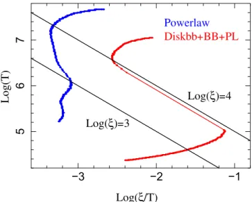
In XSTAR we simulated plasmas illuminated by different types of ionizing spectra across the 1 eV to 100 MeV energy range, including a generic power law(Γ = 2), and our RXTE/ PCA–Chandra HETGS GX 13+1 continuum. It is common to run XSTAR simulations with a power-law ionizing spectrum, and while LMXB spectra can be roughly approximated by a power law, it is not a physically consistent model, especially across the broad energy range in which the ion populations are generated. A more realistic ionizing spectrum based on our continuum model included a multicolor disk, a blackbody plus a high-energy power-law component that is cut-off below the blackbody temperature.
From the XSTAR output we generated thermal stability curves (log( )Tx versus log( )T ) for different ionizing spectra,
shown in Figure6. Portions of the thermal stability curves with negative derivatives correspond to unstable solutions. It is generally agreed that one does not expect to observe ion signatures corresponding to plasmas with temperatures and ionization parameters along the unstable branch. This phenom-enon has been invoked to explain the absence of ionized absorption features in BH LMXBs’ hard state spectra. Unstable solutions correspond to a large range of unstable ionization parameters (3.55logx4.2). This range happens to correspond with the peak fractions of many H-like and He-like ion species, making them essentially unobservable, which is in agreement with the absence of disk wind absorption Figure 5.Combined HEG± 1 orders for the five TE mode observations. Rest
wavelengths of the MnXXVand CrXXIVKα transitions are indicated by the dashed vertical lines. No MnXXVabsorption is observed, while a chromium
absorption feature can be found at a blueshift of approximately 700 km s−1. Figure 6.curve) generates a plasma with a significantly higher temperature than aThermal stability curves for two ionizing spectra. A power law(blue thermal ionizing spectrum(red curve). The black lines are lines of constant ionization parameter(logx =3, 4 for bottom/top, respectively); the thermal stability curves span ionization parameters2logx5, and both simulated plasmas have densities of 1012cm−3.
features observed in the hard state (Chakravorty et al. 2013; Bianchi et al.2017).
From Figure 6it is obvious that the nonthermal power-law ionizing spectrum produces very different plasma behavior (blue curve), occupying a temperature domain hotter for any given ionization parameter compared to a realistic thermal ionizing spectrum(red curve). As GX 13+1ʼs spectrum did not change significantly between any of the observations, the ionizing spectrum input into XSTAR is essentially the same from one observation to another. To aid in comparing differences in warmabs parameters between observations, we used the population file generated with the ObsID 11815 ionizing spectrum in all of our warmabsfits.
3.4. Warm Absorber Fits
In our warmabs modeling, we allowed for warm absorber column densities between NH= 10
20–24cm−2, ionization para-meterslogx = 2.5 5.0, outflow and turbulent velocities in the– range of 0–1500 km s−1. Infits with a single warm absorber, we were able to constrain the broad emission feature, but to reduce the number of variable parameters, we froze the broad emission parameters to the values found in Table 3.
We found our warmabs fits depended significantly on our incident ionizing spectrum. For a powerlaw ionizing spectrum, one absorber could produce all seven accretion disk wind absorption features at their observed line widths and depths, while a more physically motivated ionizing spectrum of an accretion disk, blackbody plus high-energy power law required multiple absorbers to produce all seven major features, unless we allowed for non-standard abundances.
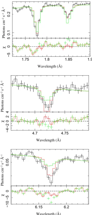
With an ionizing spectrum based on extrapolating the 1.4–40 keV Chandra and RXTE continuum model, a single warmabs component can produce absorption close to the observed levels, but the correct FeXXV/FeXXVI ratio is not produced, and the turbulent velocities(WA vturb<200 km s−1) are a fraction of the values computed from our Gaussian fits (FWHM⟹vturb≈500 km s−1). Fit parameters for a single warmabs component are shown in Table 5. The warmabs fit with a variable turbulent velocity is shown in red in Figure7; the lower ionization energy lines are visibly too narrow. We found this issue arose in all of the observations whenfit with a single warmabs component if standard abundances were assumed.
We calculated an average turbulent velocity for each observation based on our Gaussianfits to the SXVIand SiXIV
features as they are the strongest absorption lines in the portion of the spectrum with the highest spectral resolution. Fixing the warmabs vturb parameter to our Gaussian velocity widths, the high-ionization parameters required to produce the iron lines (logx »4.1) significantly under-fit the sulfur, silicon, and magnesium lines. Additionally, the cn2 values are significantly worse with the vturbparameterfixed. In Figure7, the warmabs fit with a single absorber with a fixed turbulent velocity is shown in green.
All of the aforementioned warmabs modeling have assumed standard Wilms solar abundances(Wilms et al. 2000), except
for calcium, which is required to vary in all warmabsfits. If we allow the warm absorber’s abundances to vary (in addition to calcium’s), one absorber can provide reasonable fits to all of the absorption features and match the expected turbulent broadening; details of the fits are listed in Table5. Allowing only the iron abundance to vary requires iron abundances 30% relative to solar, although the iron abundances are not
consistent between observations and the SiXIVabsorption line is still underfit. With the iron abundance relative to solar fixed to unity and allowing the calcium, argon, sulphur, silicon, and magnesium (i.e., the other major absorption feature elements) abundances to vary, requires overabundances (2–6)× solar values, but provides a better fit than allowing only the iron abundance to vary. We acknowledge that a single absorber with super-solar Ca, Ar, S, Si, and Mg abundances is a possible solution to the absorption complex modeling, but we continued to search for solutions with fewer variable abundances,finding that multiple absorption zones were required.
The FeXXVIabsorption feature’s large EW (30–45 eV) and, in particular, its width relative to FeXXV, was the first indication that a warm absorber with ionization parameter
x
log 4 is present in GX 13+1ʼs spectrum. All accretion disk wind LMXBs show absorption lines from FeXXV and/or FeXXVI, which can be modeled by photoionized plasmas with
x
log 3. Unlike most BH and NS disk wind sources where only iron lines are observed, GX 13+1ʼs spectrum exhibits significant absorption from ions with lower ionization para-meters (for example, the SiXIV Kα absorption line is at ≈2 keV with EWs of 1.2–2.9 eV), indicating a less ionized plasma is also present.
Adding more warmabs components, we found the narrow absorption features could be successfully modeled with two or three warm absorbers, see Table 6. In both scenarios, the calcium and magnesium abundances were allowed to vary in order for their full EWs to be modeled. Fitting with two warmabs components, the iron lines are associated with a highly ionized absorber (logx »4.1, NH,22≈10–20), while the silicon, sulfur, magnesium, calcium, and argon lines are partially produced by a much less ionized absorber (logx »2.9, NH,22≈0.3–0.8). The two components exhibit similar turbulent velocities(vturb≈100–800 km s−1), while the more highly ionized absorber has a larger blueshift (voutflow≈750–1150 km s−1) than the less ionized component (voutflow≈300–800 km s−1).
In a model with three warmabs components, which may not be a unique solution, one highly ionized absorber (logx »4.25, NH,22≈20–30) generates almost exclusively FeXXVI Kα absorption, a second absorber (logx »3.5, NH,22≈0.1–0.4) produces significant FeXXV absorption along with some of the lower energy lines (SXVI, SiXIV, etc.) and a third absorber produces (logx »2.95, NH,22≈0.4–0.8) the rest of the SXVI, SiXIV,and MgXIIabsorption features. Similar to ourfindings with a two-warmabs-component model, the component associated with the FeXXVIline had a larger blueshift (vout= 800–1200 km s−1) than the two components associated with the lower ionization lines (vout= 350–800 km s−1). For both the two- and three-warmabs-component solutions, we find the lowest ionization component (logx »2.9) produces SiXIII absorption around 1.865 keV (6.65 Å) in the silicon edge, as predicted by Schulz et al. (2016).
For the three warmabs fits, we assessed the error bars by performing a Markov chain Monte Carlo (MCMC) analysis using a code implemented for theISIS package based upon the methods described in Foreman-Mackey et al.(2013). (See
the description of thisISIS script in Murphy & Nowak2014.) We evolved a set of 320“walkers” (10 per free parameter in the fit) until the MCMC probability distributions reached equili-brium, as judged by the parameter probability histograms from thefinal quarter of steps in the chain being nearly identical to the probability distributions from the third quarter of chain 10
Table 5
Single warmabs Component Fits
ObsID NH,22 logx vturb vout Caa Fe Ar Si S Mg cn2(dof)
(km s−1) (km s−1)
vturbParameter Free
2708 25.9± 1.1 3.91± 0.02 200± 20 630± 30 1.77± 0.28 K K K K K 1.170(6043)
11815 26.2± 1.8 3.92± 0.01 100± 40 650± 70 1.97± 0.35 K K K K K 1.148(5966)
11816 25.6± 3.0 4.17± 0.05 210± 10 990± 50 1.98± 0.79 K K K K K 1.158(5935)
11814 15.1± 1.4 3.90± 0.04 135± 20 540± 50 1.50± 0.68 K K K K K 1.145(5827)
11817 24.8± 1.8 3.93± 0.01 130± 30 500± 60 1.27± 0.41 K K K K K 1.153(5879)
vturbParameter Fixed
2708 28.3± 2.6 4.04± 0.06 499* 740± 40 3.36± 0.65 K K K K K 1.214(6044) 11815 15.6± 1.1 3.92± 0.03 490* 840± 40 3.23± 0.61 K K K K K 1.178(5967) 11816 16.1± 1.4 4.15± 0.08 555* 870± 10 3.39± 1.17 K K K K K 1.165(5936) 11814 14.1± 1.1 4.08± 0.04 481* 820± 70 4.12± 1.16 K K K K K 1.157(5828) 11817 14.8± 1.4 3.96± 0.01 265* 570± 50 2.26± 0.82 K K K K K 1.181(5880) Fe Abundance Free 2708 39.9± 2.3 3.96± 0.02 200± 40 620± 30 1.73± 0.28 0.64± 0.11 K K K K 1.175(6042) 11815 34.9± 1.1 3.95± 0.03 150± 30 740± 10 1.77± 0.32 0.58± 0.26 K K K K 1.154(5965) 11816 27.7± 4.2 4.14± 0.06 640± 200 1050± 60 1.91± 1.00 0.55± 0.14 K K K K 1.160(5934) 11814 28.4± 1.6 3.98± 0.05 420± 80 620± 60 1.38± 0.43 0.33± 0.05 K K K K 1.142(5826) 11817 32.0± 1.8 3.96± 0.02 150± 10 480± 30 1.07± 0.33 0.46± 0.07 K K K K 1.152(5878)
Ar/S/Si/Mg Abundances Free
2708 24.7± 1.3 4.13± 0.03 400± 40 680± 30 4.99± 0.88 K 2.9± 0.8 4.4± 0.5 3.0± 0.4 3.2± 1.0 1.164(6040) 11815 20.9± 1.1 4.10± 0.03 400± 40 780± 40 5.22± 0.91 K 3.0± 0.9 4.4± 0.4 3.0± 0.4 2.6± 0.9 1.148(5962) 11816 18.0± 1.6 4.22± 0.06 680± 160 1030± 60 3.85± 1.51 K 3.8± 1.5 4.1± 0.9 2.2± 0.8 <1.3 1.154(5931) 11814 13.7± 1.3 4.14± 0.05 570± 120 630± 60 4.92± 1.58 K 1.5± 1.8 6.4± 1.0 3.2± 0.8 5.5± 1.9 1.134(5824) 11817 21.7± 1.5 4.22± 0.03 210± 10 520± 30 3.71± 1.21 K 3.6± 1.1 5.9± 0.7 3.4± 0.6 3.2± 1.3 1.140(5875) Note. a
Calcium overabundance required in all warmabsfits.
11 Astrophysical Journal, 861:26 (17pp ), 2018 July 1 Allen et al.
steps; 90% confidence level error bars were then calculated from the parameter probability distributions using the final third of chain steps.
3.5. Variability and the RXTE CD
Accretion disk wind absorption line variability, attributed to changes in accretionflow, has been seen on both short (≈ks) and long (days → months) timescales. On timescales down to tens of seconds, Neilsen et al. (2011) correlated dramatic
cyclical changes with a period of ≈50 s in the illuminating continuum to changes in the accretion disk wind column density in GRS 1915+105. On timescales of tens of ks in GRS 1915+105, Lee et al. (2002) found changes in the accretion
diskflux and the accretion disk wind density drive changes in the iron absorption features.
In previous analyses of GX 13+1, variability has been claimed on day and kilosecond timescales(Ueda et al. 2004; Díaz Trigo et al. 2012). While Sidoli et al. (2002) found no
significant changes on day timescales in the FeXXV and FeXXVI Kα EWs, Díaz Trigo et al. (2012) found significant
correlations between the hard flux (6–10 keV) and the ionization state and column density of the absorber in their five XMM/EPIC observations, which were taken days to weeks apart from one another. Ueda et al.(2004) claimed variability
in the absorber’s ionization on timescales of 5 ks in the 2002 HETGS observation of GX 13+1; changes in the iron lines’ ratio appeared to be correlated with the continuumflux.
We compared our measured wind properties with GX 13 +1ʼs position along its Z tracks, which are plotted in Figure1. All of the Chandra observations occurred while GX 13+1 was on the NB and HB; blueshifted absorption features detected in all of these observations suggests these branches are both strongly associated with an accretion disk wind. Strong radio emission commonly associated with jets has also been observed at the vertex of the NB and HB along one of the Z tracks (Homan et al.2004), which suggests accretion disk winds and
jets can be simultaneous in LMXBs and is the subject of the work of Homan et al.(2016).
During several of the Chandra observations, GX 13+1 exhibited significant movement along the CD. While the GX 13+1 light curves do not suggest significant changes or trends in the source’s intensity during the observations despite the known motion along the Z track, we investigated whether the accretion disk wind exhibits variability on small timescales as reported by Ueda et al. (2004) by breaking the observations
into 10 ks time segments, the minimum amount time required to achieve meaningful constraints on theflux and EWs.
For each time segment, we fit the Chandra HETGS data with a continuum model, simple_gpile2[tbnew×(warmabs× (diskbb+bbodyrad+powerlaw))+emission-absorption], where the emission is the broad Gaussian emission frozen to the values in Table 3, and the absorption is the FeXXVI and FeXXV narrow Gaussian features. We plotted the power-law normalization as a function of the RXTE orbit and did notfind significant variability within any observation, allowing us to fix the power-law normalization to the values in Table2. We calculated the FeXXVIand FeXXVKα lines’ EWs and plotted them against the hard 8–10 keV flux in each 10 ks segment (see Figure8).
Figure 7. ChandraHETGS data for ObsID 11815 shown in black for the iron line region(top), SXVI(middle), and SiXIVabsorption features. The warmabs model in red shows afit with a single absorber and variable turbulent velocity; the iron lines are well fit, but the absorber has a small turbulent velocity (vturb≈120 km s−1) and the predicted sulfur and silicon lines are too narrow.
In green, we plot the resultingfit when the warmabs vturbparameter isfixed to
the turbulent velocity value calculated from the Gaussian linefits (490 km s−1); the produced sulfur and silicon absorption is far below what is observed. These results demonstrate that at least two absorbers are required tofit the iron, sulfur, and silicon lines to match their observed velocity-broadened widths and EWs, unless non-standard abundances are allowed.
12
Table 6
Multiple warmabs Component Fits
ObsID NH,22(1) logx ( )1 vturb(1) vout(1) Mga NH,22(2) logx ( )2 vturb(2) vout(2) Caa NH,22(3) logx ( )3 vturb(3) vout(3) Caa cn2(dof)
(km s−1) (km s−1) (km s−1) (km s−1) (km s−1) (km s−1)
Two warmabs Components
2708 0.8± 0.1 2.98± 0.03 290± 80 570± 40 0.52± 0.22 22.1± 1.8 4.10± 0.04 600± 140 860± 60 5.35± 1.11 K K K K K 1.143 (6032) 11815 0.6± 0.1 2.92± 0.01 380± 110 630± 60 0.34± 0.19 17.7± 0.7 3.99± 0.02 410± 20 910± 50 4.07± 0.70 K K K K K 1.132 (5962) 11816 0.3± 0.1 2.86± 0.10 250± 210 790± 110 0.28± 0.25 17.8± 1.5 4.21± 0.05 820± 190 1170± 80 3.80± 1.71 K K K K K 1.141 (5924) 11814 0.5± 0.1 2.71± 0.05 260± 110 310± 50 0.59± 0.22 12.5± 1.3 4.07± 0.05 380± 90 960± 80 4.48± 1.63 K K K K K 1.111 (5816) 11817 0.7± 0.1 2.88± 0.07 60± 130 400± 60 0.31± 0.21 13.5± 1.3 4.05± 0.05 400± 150 760± 70 3.32± 1.20 K K K K K 1.120 (5870) Three warmabs Componentsb
2708 0.8± 0.1 2.94± 0.1 340± 510 590± 320 0.44± 0.3 0.2± 0.1 3.57± 0.11 340c 590c 5.60± 1.65 30.4± 12.1 4.25± 0.10 630± 370 890± 60 5.60d 1.146 (6031) 11815 0.7 3.01 390 640 0.35 0.1 3.50 390 640 4.55 32.2 4.21 420 960 4.55 1.139 (5961) 11816 0.4 2.93 420 790 <0.50 0.2 3.39 420 790 3.60 19.2 4.25 850 1190 3.60 1.149 (5923) 11814 0.7 3.03 390 390 0.65 0.1 3.45 390 390 6.11 20.1 4.32 630 1030 6.11 1.116 (5815) 11817 0.7 3.03 130 480 0.33 0.2 3.46 130 480 3.69 22.1 4.31 420 840 3.69 1.136 (5869) Notes. a
Variable calcium and magnesium abundances are required. b
The 90% error bounds for the three warmabsfits were estimated with Markov chain Monte Carlo runs. Bounds for the other observations are similar to those stated for ObsID 2708. c
The turbulent and blueshift velocities were tied between the WA(1) and WA(2) components for the 3 warmabs components model. d
The WA(2) and WA(3) calcium abundances were tied.
13 Astrophysical Journal, 861:26 (17pp ), 2018 July 1 Allen et al.
Overall, both the FeXXVI and FeXXV EWs exhibit a correlation with the 8–10 keV flux; as the hard flux increases, the EWs decrease. Looking at individual observations, the hard flux evolves across the 10 ks segments as expected with their movement along the CD(see Figure1). For example, in ObsID
11817 GX 13+1 moves along its Z track from the NB/HB vertex to the NB/FB vertex, during which both the soft and hard colors decrease. In Figure8, GX 13+1 can be found in the first 10 ks of the observation with an 8–10 keV flux of 5.2×10¹⁰erg s−1cm−2; the hard flux decreases throughout the observation as the FeXXVIand FeXXVEWs both increase. The FeXXVIEW increases by over 50% while the FeXXVEW nearly doubles.
In a disk wind model where two absorbers are present, one absorber produces both of the Fe Kα lines. The EW ratio (FeXXV EW/FeXXVI EW) is a probe of the ionization state. The errors in the EW ratios, however, are too large to interpret relative changes in the absorption features during any of the observations. The apparent correlation between both the iron lines’ EW and the 8–10 keV flux does not support a change in the ionization state. For both the FeXXVIand on FeXXVEWs to decrease with the hardflux, the ionization state must remain remain constant while the wind column density decreases. If one absorber produces the FeXXVI line and another produces the FeXXVline, as is the case in our three-absorber model, the trend could be produced by several scenarios involving changes in both the ionization states and/or the column densities.
4. Discussion
As the number of high-resolution observations of disk wind systems has grown over the past decade, it has become increasingly clear that disk winds play a critical role in the overall accretion process in both BH and NS LMXBs. GX 13 +1 is one of only three NS narrow absorption line systems that
shows a definitive outflow; IGR J17480-2446 (Miller et al. 2011) and Cir X-1 (Brandt & Schulz 2000) are the
others. In contrast, all BH narrow line systems exhibit blueshifts (Díaz Trigo & Boirin 2016). GX13+1 is bright,
accreting at more than 50% Eddington and displays seven major absorption features, the most among NS disk wind systems, revealing a detailed view of the absorbing plasma’s properties. Its simultaneous Chandra HETGS and RXTE/PCA observations offer the unique chance to study the disk wind properties along the source’s horizontal and normal branches.
The abundance of high-S/N observations of GX 13+1 allowed us to perform a detailed analysis of the disk wind absorption spectrum in GX 13+1. We have fit the Chandra and RXTE1.5–40 keV spectrum and performed direct line fits of the seven strongest absorption features, including hydrogen-and helium-like iron Kα lines and the Kα lines from hydrogen-like Ca, Ar, S, Si, and Mg. Through careful photoionization modeling of the absorption features, we found multiple absorbers were required to produce the observed disk wind signature, unless nonstandard abundances were assumed.
4.1. Multiple Absorbers in Accretion Disk Winds Previous analyses of the accretion disk wind in GX 13+1 required only one warm absorber, while we find at least two absorbers are necessary. The disagreement may be a result of inherent variability or our improved treatment of the ionizing spectrum. In the five XMM observations Díaz Trigo et al. (2012) found significant absorption due to the Kα and Kβ
transitions of FeXXVand FeXXVI. Evidence of absorption due to the lower-energy transitions in SiXIV, SiXIII, SXV, SXVI, and CaXXwere present in several observations. The measured EWs were compatible with a single, highly ionized absorber with logx =4 (Díaz Trigo et al. 2012). If only one absorber
was indeed present in the XMM observations, it would indicate variability in the wind’s ionization state, as the lower-ionization components we see in our Chandra observations are absent. However, the low energy resolution of the XMM/EPIC observations makes the detection of the narrow, less ionized absorption features unlikely even if they were present.
In the bestfits to our data, we found at least two absorption zones with different ionization parameters and outflow velocities were required to produce the observed disk wind signature. Multiple absorbers have been seen in disk wind systems before. Evidence of multiple velocity components was seen in LMXB BH GRO J1655-40 (Kallman et al. 2009; Neilsen & Homan2012). Taking a closer look at the iron line
region (6–8 keV) in the third-order HEG spectra of four BH disk wind systems, including GRO J1655-40, Miller et al. (2015) found fits with two or more absorption zones,
significantly improved their fits.
Specifically, among NS systems with narrow line absorption features, multiple absorption zones are not uncommon; three have one low-ionization component (logx <3) and one high-ionization component (logx >3) (Díaz Trigo & Boirin
2016). Absorption features associated with ions observed in
GX 13+1ʼs spectrum, including SXVI, SXIV,and MgXII, have also been observed in the NS binaries 4U 1916-05 and Cir X-1. In 4U 1916-05, an accretion disk atmosphere source, the FeXXV and FeXXVI features were produced by an absorber with logx »4.15 while the S, Si, Mg, and Ne lines were associated with a much less ionized component, logx »3 (Iaria et al.2006). Similarly, in GX 13+1 we found absorption
Figure 8. FeXXVI (star symbols) and FeXXV (filled circles) EWs vs. the 8–10 keV flux in 10 ks time steps of each of the five TE mode observations. The change in hardflux during the course of the observation roughly reflects the source’s motion along its Z track. In ObsID 11816, GX 13+1 occupies a relatively small area at the HB/NB vertex, which is reflected in the small range of its 8–10 keV flux across the time segments.
14
zones withlogx =2.9 3.5 produced the less ionized features.– While the absorption features in Cir X-1 were very broad (FWHM≈2000 km s−1 compared to the 400–600 km s−1 we observe in GX 13+1), they exhibited strong P-Cygni profiles, supporting the interpretation that the lines are due to an accretion disk wind (Brandt & Schulz 2000; Schulz & Brandt 2002).
Observing multiple absorption zones in an accretion disk wind will provide multiple measurements of the plasma’s outflow velocities and ionization parameters and will help probe the disk wind structure and, hence, the wind launching mechanism. Our analysis highlights the importance of not using an approximated ionizing spectrum, such as a power law, in the XSTAR analysis. A re-analysis of the warm absorber modeling in disk wind sources may reveal multiple absorption components previously not identified. Future X-ray instruments with higher energy resolution and larger effective area will allow us to see more and more absorption line components, as weak lines become visible and blended lines become resolved (Kallman et al.2009).
In disk wind and disk atmosphere systems where multiple absorbers provide the best fit the to absorption line complex, the absorption zones are usually typified by distinct ionization states or by outflow velocity. In GX 13+1, the absorption zones differ by the associated column, ionization state, and velocity. These multiple absorption zones may be a natural signature of a smooth outflow. Simulations of Compton-heated winds suggest the absorption line complex may be character-ized by two or three ioncharacter-ized zones (Giustini & Proga 2012; Higginbottom & Proga 2015). Alternatively, the different
ionization zones may correspond to “clumps” of outflowing material, challenging the assumptions of a continuous and homogenous outflow. In this scenario, one might expect strong temporal variability in the absorption line features due to the noncontinuous outflow of absorbing material. As we see the same absorption features in all seven observations that span almost 10 years of monitoring, and model the absorption zones with similar ionization parameters and column densities, this suggests a relatively continuous and smooth outflow as opposed to large, separate physical clumps of outflowing material.
4.2. Disk Wind Launching Mechanism
Compton heating and magnetic driving are considered the most viable mechanisms in X-ray binary disk wind systems. For several BH wind systems (e.g., GRO J1655-40 and GRS 1915+105), there have been claims of magnetic driving based on small inferred wind launching radii (Miller et al. 2006,
2016b, but see also Neilsen et al.2016and Shidatsu et al.2016
for an alternative explanation). Unusual wind properties or changes in wind properties within a single outburst have also driven the formulation of hybrid wind theories (Neilsen & Homan2012).
Previous studies of the disk wind in GX 13+1 have found that it is consistent with Compton heating (Sidoli et al.2002; Díaz Trigo et al.2012; Madej et al.2014), although Ueda et al.
(2004) proposed radiation-driven wind based on a model where
radiation driving could be effective at sub-Eddington luminos-ities. The question of the wind launching mechanism in any disk wind system is often answered by determining the wind launching radius (R = Lx
n
L ); this is approximated as the
radius where we observe the innermost absorption region which is estimated from the definition of the ionization parameter (Equation (1)). As previously discussed in
Section3.3.1, the largest uncertainty in disk wind observations is the plasma density. It is also the largest uncertainty in determining the wind launching radius and, hence, the wind mechanism. We have no independent measurement of the plasma density in GX 13+1, so for this reason and for consistency we use the same electron density we used to calculate our population levels in XSTAR, n= 1012cm−3.
Uncertainty in the bolometric luminosity is the second largest source of error in determining the wind launching radius. The bolometric luminosity is estimated from the X-ray luminosity, which can be significantly underestimated when there is a high opacity along the line of sight, the exact conditions when observing highly inclined disk wind systems (Díaz Trigo & Boirin 2016). While there is a large neutral
column density (NH,22>1) toward GX 13+1, as well as a warm absorber with an even larger column density (NH,22≈30), we benefit from simultaneous RXTE observa-tions in estimating a broadbandflux. Homan et al. (2016) found
that GX 13+1 was accreting at nearly its Eddington limit, L = (1.2–1.3)×1038
erg s−1 (≈0.7–0.8 LEdd) across 0.1–100 keV, while in this work we estimated slightly lower Eddington fractions (≈0.45 LEdd), in part because we did not include the power-law flux below ∼2.5 keV. Both estimates of the bolometric luminosity are likely a lower bound because the accretion disk’s flux has not been corrected for inclination and because of the luminosity suppression associated with the source’s high obscuration, as previously mentioned. The highest ionization parameter we detected in our observations of GX 13+1 was logx »4.3. Rewriting the launching radius in terms of our estimates for the density and luminosity, wefind
x = ´ ´ ´ ´ ´ -⎜ ⎟ ⎛ ⎝ ⎜ ⎞ ⎠ ⎟ ⎛ ⎝ ⎞ ⎠ ⎛ ⎝ ⎜ ⎞ ⎠ ⎟ R L n 7 10 1.3 10 erg s 10 cm 10 erg cm s cm. L 10 38 1 12 3 4.3 1 1 2 1 2 1 2
Our launching radius is consistent with other published estimates, RL≈1010–11cm (Ueda et al. 2004; Díaz Trigo et al.2012; D’Aì et al.2014), despite the variety of luminosities
and densities used to estimate the radius. Compton-heated winds can be launched outside of the 0.1×Compton radius, RC (Begelman & McKee1983). The Compton radius, RC, is given by: = ´ ´ - ⎜ ⎟ ⎛ ⎝ ⎜ ⎞ ⎠ ⎟ ⎛⎝ ⎞⎠ ( ) R M M T 10 10 K cm, 2 C 10 NS C 8 1
where MNSis the NS mass and TCis the Compton temperature defined as:
ò
ò
n n n = n n ¥ ¥ ( ) T k h L d L d 1 4 . 3 C B 0 0From our Chandra observations, we calculate a typical Compton temperature of 1.3×10⁷K (see the red curve in Figure6), which translates to a Compton radius of 8×1010cm and is comparable with our wind launching radius. As a Compton-driven wind can be launched just beyond 0.1 RC, this